Sharif University of Technology
Scientia IranicaTransactions A: Civil Engineering http://scientiairanica.sharif.edu
An eective approach to structural damage localization
in exural members based on generalized S-transform
H. Amini Tehrani
a, A. Bakhshi
a;, and M. Akhavat
ba. Department of Civil Engineering, Sharif University of Technology, Tehran, P.O. Box 11155-9313 Tehran, Iran. b. School of Civil Engineering, Iran University of Science & Technology, Tehran, Iran.
Received 7 February 2017; received in revised form 22 October 2017; accepted 23 December 2017
KEYWORDS Damage localization; Signal processing; Generalized S-transform; Time-frequency representation; Non-stationary signals.
Abstract. This paper presents a method for structural damage localization based on signal processing using generalized S-transform (SGS). The S-transform is a combination
of the properties of the Short-Time Fourier Transform (STFT) and Wavelet Transform (WT) that has been developed over the last few years in an attempt to overcome inherent limitations of the wavelet and short-time Fourier transform in time-frequency representation of non-stationary signals. The generalized type of this transform is the SGS-transform
that is characterized by an adjustable Gaussian window width in the time-frequency representation of signals. In this research, the SGS-transform was employed due to its
favorable performance in the detection of the structural damages. The performance of the proposed method was veried by means of three numerical examples and, also, the experimental data obtained from the vibration test of 8-DOFs mass-stiness system. By means of a comparison between damage location obtained by the proposed method and the simulation model, it was concluded that the method was sensitive to the damage existence and clearly demonstrated the damage location.
© 2019 Sharif University of Technology. All rights reserved.
1. Introduction
Structural health monitoring has become an evolving area during the recent years with an increasing need to ensure the safety and functionality of structures. It can be stated that the importance of structural health monitoring lies in the serviceability and safety of struc-tures during their service life; of course, appropriate and timely actions are required for their maintenance and retrotting. In the past few decades, using signal processing tools in structural health monitoring has
*. Corresponding author. Tel.: +98 21 66164243;
E-mail addresses: aminitehrani [email protected] (H. Amini Tehrani); [email protected] (A. Bakhshi);
[email protected] (M. Akhavat). doi: 10.24200/sci.2017.20019
increased considerably due to the recent advances in the eld of sensors and other electronic technologies [1]. These advances provide a wide range of response signals such as velocity, acceleration, and displace-ment caused by low- to high-intensity earthquakes and environmental loads. Doubling et al. [2] provided a comprehensive history of structural health monitoring methods together with eciencies and disadvantages of each method. Sohn et al. [3] presented comprehensive literature reviews of vibration-based damage detection and health monitoring methods for structural and mechanical systems.
Signal-based methods investigate changes in the features derived from the series or their corresponding spectra using proper signal processing tools. One of the most commonly used signal processing techniques is the Fast Fourier Transform (FFT), which transmits signals from the time domain into the frequency domain. In
other words, the evaluation of the FFT of a signal results in a graph in the frequency domain by taking into account the average size of each spectral amplitude assessed on the entire length of the analyzed signal. It is evident that the transient phase of the signal, which appears to be a fraction of the whole signal, is entirely distorted [4]. Therefore, the FFT is not a proper tool for processing non-stationary signals. The non-stationarity of the recorded signals is not merely due to the damage to structures; even the non-stationarity of the input and the possible inter-action with the ground or adjacent structures can show the ineectiveness of classic techniques [5]. A large number of researchers have developed methods for overcoming the above-mentioned problems of the FFT in processing non-stationary signals. The short-time Fourier transform [6,7], the complex demodulation technique [8], and the Generalized Time-Frequency Distribution (GTFD) as proposed by Cohen [9] are examples of these methods.
In recent years, extensive research has been car-ried out in the eld of structural health monitoring by utilizing the decomposing features of wavelet and wavelet packet transforms. Ovanesova and Suarez [10] used the wavelet transform to detect cracks in a one-story plane frame. They investigated the eec-tiveness of wavelet analysis in detecting cracks by using numerical examples. Ren and Sun [11] used a combination of wavelet transform and Shannon entropy to detect structural damage from vibrational signals. They used wavelet entropy, relative wavelet entropy, and time-wavelet entropy as damage-sensitive features for the detection and determination of the damage location. Several recent studies investigating wavelet-based methods can be found in [12-15].
Wavelet and wavelet packet transforms have some imperfections such as unavailability of the width of time-frequency window for all frequencies, which is in-evitable for having windows with adjustable width [16]. These transformations present more advantages than the FFT and the STFT, yet do not allow for a fair assessment of the local spectrum. In other words, these instruments are incapable to perform a correct evaluation of the spectral characteristics, considering the instantaneous variations [4].
Stockwell et al. [17] introduced a new trans-form (S-transtrans-form) that combines the characteris-tics of Short-Time Fourier Transform (STFT) and wavelet transform. Unlike the wavelet transform, the S-transform preserves phase-referenced information. This transform has been used by some researchers in various elds such as seismology [18,19]. In structural health monitoring, for the rst time, Pakrashi and Ghosh [20] used the S-transform to detect cracks in beams. Ditommaso et al. [21,22] introduced a lter based on S-transform to process the response signals,
considering the evolution of dynamic characteristics of structures with time. Ditommaso et al. [23] recently developed a methodology for damage assessment and localization of framed structures subjected to strong-motion earthquakes. In this method, the information related to the evolution of the equivalent viscous damping factor and mode shape is extracted from the recorded signal using a band-variable lter and Stock-well Transform. Then, based on the fundamental mode shapes evaluated before, during, and after the seismic event, the modal curvature variation is quantied, and damage location is identied.
With all the advantages over all other transforms, such as wavelet and short-time Fourier transform, the S-transform also has some disadvantages one of which is an invariable window that has no parameter for allowing its width to be adjusted in the time or frequency domain. To overcome this problem, the generalized S-transform is introduced with adjustable time and frequency resolution.
In this paper, the generalized S-transform is pre-sented to detect the presence and location of damage in structures. Herein, the rst wavelet transform and S-transform are presented; then, their dierences in the time-frequency representation signal are expressed in the form of a simple example. Afterward, the generalized S-transform is introduced, and the damage detection procedure is explained by taking advantage of this transform. The eciency of the proposed method for damage detection is examined with respect to three dierent numerical examples. Furthermore, the experimental data from the vibration test of a mass-stiness system are used to verify the proposed approach. The results reveal that the proposed method is robust and ecient for the detection and localization of damage.
2. Signal processing tools 2.1. Wavelet transform
The wavelet transform is a method for converting a signal into another form, which either makes certain features of the original signal more amenable to study or enables the original dataset to be described more succinctly. There are, in fact, a large number of wavelets to choose from for data analysis. The best one for a particular application depends on both the nature of the signal and what we require from the analysis [24]. The wavelet transform of a continuous signal, f(t), can be expressed as follows [25]:
W (a; b) =p1 jaj Z +1 1 f(t) t b a dt; (1) where a and b are the scale and the transformation parameter, respectively.
of a;b. Function a;b(t) is obtained from Function (t)
(mother wavelet) by scale a and transformation in the time domain using b.
2.2. S-Transform
The S-transform produces a time-frequency representa-tion of a time series. It uniquely combines a frequency-dependent resolution with simultaneous localization of the real and imaginary spectra. This transform was introduced by Stockwell et al. [17].
The continuous S-transform of function h(t) with Gaussian window is dened as follows:
S(; f) = Z 1
1h(t)fw( t; f)e
i2 ftgdt; (2)
where the Gaussian window (w) is dened as follows: w( t; f) = pjfj
2exp "
f2( t)2
2 #
: (3)
In Eq. (2), a voice S(; f0) is dened as a
one-dimensional function, of time for a constant frequency f0, which shows how the amplitude and phase for this
exact frequency change over time. A `local spectrum' of S(0; f) is a one-dimensional function of frequency
for a xed time, t0, [16].
The Gaussian window is chosen due to the follow-ing reasons [16]:
1. It uniquely minimizes the quadratic time-frequency moment about a time-frequency point;
2. It is symmetric in time and frequency. The Fourier transform of a Gaussian function is Gaussian;
3. By using it, none of the local maxima in the absolute value of the S-transform is an artifact.
The width of the Gaussian window changes with 1=jfj. This change creates distributions with dierent time-frequency resolutions. However, the value of 1=jfj is constant, and the width of the window cannot be adaptively adjusted to the frequency distribution of the signal.
The S-transform uses a window with variable widths so that the time window can be wider at the low-frequency band to gain higher frequency resolution. On the contrary, the time window is narrower at the high-frequency band to obtain higher time resolution. In this respect, is the center of the window and deter-mines the location of the Gaussian window at time axis. Both S-transform and wavelet transform have the characteristic of multi-resolution. The S-transform is similar to the wavelet transform in terms of a progressive resolution; however, unlike the wavelet transform, the S-transform retains the referenced phase information absolutely and has a frequency invariant amplitude response. Moreover, the role of phase in wavelet analysis is not as well understood as it is for the Fourier transform [16]. In addition, wavelet reconstruction leads to information leakage, while the S-transform is nondestructive and reversible.
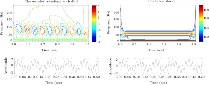
The synthetic signal shown in Figure 1 is com-posed of two sinusoidal waves with frequencies 10 and 50 Hz, respectively. The signal length is 512 ms with the sampling interval of 2 ms. Figure 1 on the left side shows the time-frequency distribution of the wavelet transform with DB6 mother wavelet function. The S-transform of the proposed signal is also shown on the right side of Figure 1. It is clear that the S-transform reects the time-frequency representation of the synthetic signal more precisely.
2.3. Generalized S-transform
The generalized S-transform is dened as follows [26]:
SSG(; f; p) =
Z 1
1h(t)fwG( t; f; p)
exp( 2ift)gdt; (4) where wG is a generalized Gaussian window. By
applying appropriate p factor to Eq. (3), wG is given
by:
wG( t; f; p) = pjfj2exp
"
p f2( t)2
2
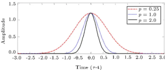
# : (5) Positive parameter p is the width factor in cen-tralizing the Gaussian window that controls the width of the Gaussian window. A sinusoidal function, as an example, with a period of 10 sec includes a Gaussian window with p 10 width. In this particular case, Eq. (2) is obtained if p = 1.
If w is an S-transform window, it must satisfy four conditions [27,28]. These conditions are [28]:
Z 1
1<fw(; f; p)gd = 1; (6)
Z 1
1=fw(; f; p)gd = 0; (7)
w( t; f; p) = [w( t; f; p)]; (8)
@
@t ( t; f; p)jt= = 0: (9) The rst two conditions ensure that, when integration is carried out over all , the S-transform converges to the Fourier transform:
Z 1
1S(; f; p)d = H(f): (10)
The third condition can ensure the property of symmetry between the shapes of the S-transform analyzing function at positive and negative frequencies. The above-listed conditions provide an appropriate re-lationship between S-transform and Fourier transform. In Eq. (5), if p < 1, then the Gaussian window in the time domain expands; thus, the temporal resolu-tion decreases and the frequency resoluresolu-tion increases; however, when p > 1, the reverse of the action occurs. Figure 2 shows the Gaussian window at dierent values of p and f = 3 Hz. As can be seen, by increasing the amount of p, the width of the Gaussian window in the time domain decreases.
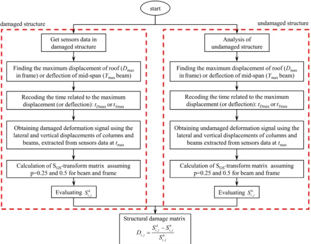
3. Generalized S-transform methodology for damage detection
The main idea of the generalized S-transform method is based on the assumption that the eect of incoming
Figure 2. Generalized Gaussian window in the time domain.
load damages produces discontinuities in the structural deformation curve such that most of these discontinu-ities are not detectable through the observation of the recorded response signals. As will be explained, the sig-nal used here is the deformation sigsig-nal of the structure as a function of the node number. Discontinuous points of the signal can be detected with high accuracy by the generalized S-transform with increasing temporal resolution and decreasing frequency resolution. This feature can be used in discontinuity detection of the deformation signal. Herein, the time axis is replaced by the number of nodes.
To detect the presence and location of damage to structures by using SGS-transform, the following
procedure is introduced:
1. The structural response signals are measured by the desired degrees of freedom in both healthy and damaged structures under applied loads. In beams the vertical, and in frames the vertical and lateral displacements are usually considered;
2. The time of the occurrence of maximum displace-ment in a healthy structure (tD max) is obtained. It
can be used as a basis of the action for damage detection. In multi-span beams, the maximum vertical displacement at the middle of spans and in frames' columns and beams, the maximum lateral and vertical displacements are employed respec-tively for detection and localization of damage;
3. The total structural deformation signal is calculated in both undamaged and damaged states. In the continuous beams, deformation signal is achieved by using vertical displacement response of all nodes in tD max . In addition, in the frame, this signal for
both lateral and vertical displacements is achieved by using calculated responses in all frame nodes in tD max;
4. The structural deformation signals are processed in both undamaged and damaged states, and SGS
-transform coecients (SGS-transform matrix) are
achieved by using generalized S-transform. In this paper, p = 0:5 and p = 0:25 are proposed for damage detection in frame and beams, respectively. This matrix includes N rows and M columns such
that M is equal to the number of nodal points, and the number of each column represents the node number in the original structure;
5. The structural damage matrix is calculated through the following equation:
Di;j= S d i;j Shi;j
Sh
i;j ; (11)
where Di;j is the element of the ith row and
jth column of the structural damage matrix. In addition, Sd
i;j and Si;jh are the absolute values of
the elements of the ith row and jth column of the SGS-transform matrices as calculated in step 4 for
both undamaged and damaged states;
6. Damage matrix elements have high sensitivity to abrupt changes and discontinuities in the defor-mation signal resulting from stiness changes in adjacent elements at high frequencies. Hence, the damage location can be determined by plotting the lower half of the damage matrix spectrum against the node numbers. These rows of the damage matrix are related to high frequencies. The owchart of the proposed algorithm is shown in Figure 3.
4. Numerical study
The capability of the S-transform in structural damage identication and localization is demonstrated through three numerical examples. Numerical examples include a 3-span continuous beam with two xed ends sub-jected to harmonic load with a resonant frequency, a 5-span continuous beam with two xed ends subjected to impact loading, and a 4-story 1-bay steel moment-resisting frame under seismic loading. The purpose of using dierent loading types is to demonstrate the capability and accuracy of the proposed algorithm to process response signals caused by applying various loading types.
In the proposed examples, since the structural performance is exural, all damage scenarios are con-sidered to experience a reduction in the bending sti-ness (EI) in percentage. Structural damping has been considered based on Rayleigh damping with = 0:05. In this section, the damage patterns in structural elements, such as beams and columns, have been selected so as to simulate the damage occurring as a result of high-cycle fatigue caused by the presence of permanent loads on the bridges (Examples 1 and 2) or low-cycle fatigue caused by earthquakes (Example 3).
4.1. Three-span continuous beam 4.1.1. Model description
A 3-span continuous beam with xed supports at both ends (A and D supports) is considered as Example 1 (Figure 4). Geometric properties of the beam are given below. The total length of the beam is 18 m with three equal spans of 6 m. The area moments of inertia and cross-section are the same regarding the entire length of the beam and are 57680 cm4and 198 cm2, respectively.
Material properties, such as modulus of elasticity and Poisson ratio, are E = 200 GPa and = 0:2, respectively. The distributed mass with the intensity of 3260 kg/m is also considered. The performance of the 3-span beam in load bearing is very similar to that of multi-span bridge with continuous deck [29]. In this example, a harmonic load with a resonant frequency is applied to excite the beam. According to the studies conducted by Alwash et al. [29], the harmonic excitation at a resonant frequency of a 3-span beam with two xed ends presents credible information for damage detection in multi-span bridges. Analysis of the beam under incoming loads is done using the nite element method in Matlab software. In this regard, the presented beam shown in Figure 4 is subdivided into 54 nite elements with equal lengths, such that each
Figure 4. Three-span continuous beam model and related nodal points.
of the end nodes of the elements has two vertical and rotational degrees of freedom.
4.1.2. Harmonic loading
To apply a harmonic load, the natural frequency of the rst mode of vibration should be calculated. The estimated value of the rst-mode natural frequency is 10.6 Hz, which is calculated via eigenvalue analysis. Therefore, the harmonic excitation characterized by the 1000 N amplitude and the frequency equal to the rst mode natural frequency is applied in the middle of the second span of the beam. The time history of the harmonic excitation is shown in Figure 5. In addition, the considered damage scenarios are listed in Table 1.
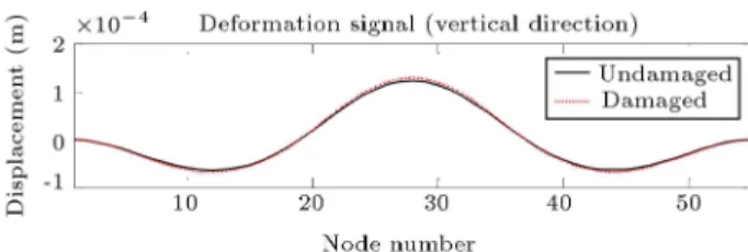
Herein, undamaged and damaged structures are analyzed under the mentioned loading condition. Fig-ure 6 represents the beam deection curve in tD max
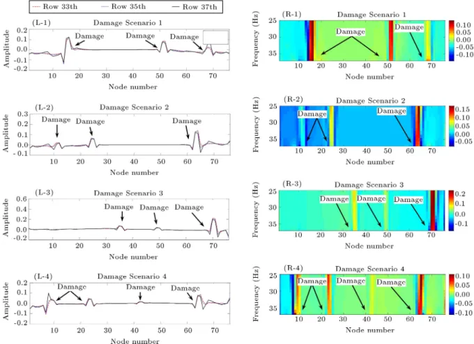
both in undamaged and damaged states for Damage Scenarios (4). The damage matrix of the beam, which is obtained from Eq. (11), includes 55 columns (the number of nodes) and 27 rows.
In Figure 7, the spectrum of rows 15 to 27 of the damage matrix is shown on the right side, and the diagrams related to the entries of rows 23, 25, and
Figure 5. Time history of the harmonic excitation at the resonant frequency.
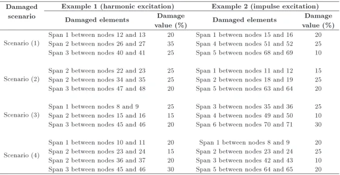
Table 1. Considered damage scenarios in the 3-span and 5-span continuous beams under incoming loads. Damaged
scenario
Example 1 (harmonic excitation) Example 2 (impulse excitation) Damaged elements Damage
value (%) Damaged elements
Damage value (%) Scenario (1) Span 1 between nodes 12 and 13Span 2 between nodes 26 and 27 2035 Span 1 between nodes 15 and 16Span 4 between nodes 51 and 52 2025
Span 3 between nodes 40 and 41 25 Span 5 between nodes 68 and 69 10
Scenario (2) Span 2 between nodes 22 and 23Span 2 between nodes 34 and 35 2525 Span 1 between nodes 11 and 12Span 2 between nodes 18 and 19 1525 Span 3 between nodes 47 and 48 20 Span 5 between nodes 63 and 64 20
Scenario (3) Span 1 between nodes 8 and 9Span 2 between nodes 15 and 16 2515 Span 3 between nodes 35 and 36Span 4 between nodes 49 and 50 2510 Span 3 between nodes 45 and 46 20 Span 6 between nodes 70 and 71 30
Scenario (4)
Span 1 between nodes 10 and 11 20 Span 1 between nodes 8 and 9 20 Span 2 between nodes 23 and 24 15 Span 2 between nodes 23 and 24 25 Span 2 between nodes 36 and 37 20 Span 3 between nodes 42 and 43 10 Span 3 between nodes 45 and 46 30 Span 5 between nodes 64 and 65 20
27 are demonstrated on the left side for all damage patterns. In Figure 7, all the horizontal axes represent the node numbers. According to Figure 7, it is observed that the location of all damaged elements has been identied with high accuracy. For example, in Damage
Figure 6. Deformation signal of the 3-span beam at tD max in Damage Scenario (4).
Scenario (4), the number of damaged elements is 4; as shown by the result, the location of damaged elements is precisely detectable.
4.2. Five-span continuous beam 4.2.1. Model description
In Example 2, a 5-span continuous beam with xed supports at both ends (A and F supports) is investi-gated (Figure 8). Geometric and material properties of the beam are the same as those of the 3-span beam, as explained in Example 1. The distributed mass with the intensity of 3260 kg/m is also considered in Example 2. To excite the beam, an impact load with a half-sine pulse is applied [29]. Analysis of the beam under incoming loads is conducted using the nite element
Figure 7. 23rd, 25th, and 27th elements (L-1 to L-4) of the damage matrix and damage matrix spectrum (R-1 to R-4) for damage scenarios in Example 1.
method. For this purpose, the beam shown in Figure 8 is subdivided into 75 nite elements with an equal length such that each node at two ends of the element has two (vertical and rotational) degrees of freedom. 4.2.2. Impact loading
The time history of the impact load is shown in Figure 9. The impact load amplitude is 100 N that is applied to the structure as a half-sine pulse within 0.05 sec. The point of action is in the middle of the third span at a distance of 3 meters from support C. The considered damage scenarios of the impact excitation are demonstrated in Table 1. The damaged and un-damaged structures are analyzed under the considered damage scenarios, and deformation curves at tD maxare
obtained for each of the patterns. Figure 10 represents the beam deection curve in tD maxboth in undamaged
and damaged states for Damage Scenarios (2). Similar to Example 1, the damage matrix is obtained through Eq. (11) for each damage pattern. The resulting damage matrix includes 76 columns and 38 rows for each of the patterns. In Figure 11, the spectrum of rows 25 to 37 of the damage matrix is shown on the right side, and the diagrams related to the entries of
Figure 9. Time history of the impact excitation.
Figure 10. Deformation signal of 5-span beam at tD max
in Damage Scenario (2).
rows 33, 35, and 37 are shown on the left side for all damage scenario. In Figure 11, all the horizontal axes represent the node number. In Example 2, according to the damage scenarios listed in Table 1, it is observed that the location of all damaged elements has been identied with high accuracy. For example, in Damage Scenario (3), the number of damaged elements is 3. According to Figure 11, the locations of damaged elements have been accurately detected.
4.3. Plane frame 4.3.1. Model description
In Example 3, a 4-story 1-bay moment-resisting frame (Figure 12) is selected to evaluate the eectiveness of the proposed method. The span length is 6 m, and the height of all stories is the same and equal to 3 m. The geometric properties of the members are represented in Table 2. The modulus of elasticity is E = 200 GPa, and the distributed mass with the intensity of 3260 kg/m is considered for all story levels. This intermediate steel moment-resisting frame is designed based on the Iranian Seismic Code (Standard 2800) -3rd edition and volume 10 of the Iranian National Building Codes for steel structure design. The earthquake lateral force eective in this frame is calculated by the equivalent static method. It is assumed that the model is located in a high relatively hazard area with 0.3 g base design acceleration and soil type III (according to Standard 2800). In addition, the occupancy importance factor of the structure is considered as moderate. In the extraction of the spectral parameters, the damping ratio is presumed to be 5%.
After the completion of the design process, the frame is analyzed in both intact and damaged states under the applied seismic load using nite-element method. In this regard, the frame shown in Figure 12 is subdivided into 120 nite elements in such a way that each element in beam and column is 0.5 m and 0.333 m, respectively. Each node at both ends of the element has vertical and rotational degrees of freedom.
4.3.2. Seismic loading and considered damage scenarios
After the occurrence of an earthquake, detecting the presence, location, and severity of damage is a major step in the assessment of structural condition. After
Table 2. The geometric properties of the members in the moment frame.
Story
Beams Columns
Cross section (mmm222)
Area moment of inertia (mmm444)
Cross section (mmm222)
Area moment of inertia (mmm444)
1st , 2nd 6.791E-3 1.507E-4 0.0216 2.639E-4
Figure 11. 33rd, 35th, and 37th elements (L-1 to L-4) of the damage matrix and damage matrix spectrum (R-1 to R-4) for damage scenarios in Example 2.
a major earthquake in a region, numerous aftershocks with low magnitude (PGA < 0:1 g) occur, which can also be said that structures at the low-intensity aftershocks will not suer any damage. Thus, it is possible to use aftershocks as an incoming excitation in the detection of the occurred damage in major earthquakes.
In Figure 13, Tabas ground motion (Sade Station) and Fourier spectrum related to this excitation are demonstrated. The considered damage scenario for seismic loading is listed in Table 3. Damaged and un-damaged structures are analyzed under the considered damage scenarios, and the deformation signals in both horizontal and vertical degrees of freedom in tD maxare
calculated.
Vertical displacement in beams and horizontal displacement in columns represent the behavior of the corresponding loading. Thus, vertical and lateral deformations in tD max are used to detect damage
in beams and columns, respectively. Vertical and lateral deformation signals in tD max are demonstrated
in Figure 14 for Damage Scenario (2). Then, according to the algorithm described above by using Eq. (11), the damage matrix is obtained for each of the damage
scenarios of the frame in both directions. Since the number of nodal points in this structure is 118, the damage matrix dimension for each of the patterns includes 118 columns and 59 rows. In Figure 15, the damage matrix spectra for detecting damages to beams are demonstrated on the right side, and the elements related to rows 55, 57, and 59 of the damage matrix are demonstrated on the left side for all damage scenarios. In Figure 15, all the horizontal axes represent the node number. According to the damage scenarios in Table 3 and Figure 15 (2, 4, 6, 8, R-10), it is observed that all the damaging elements in beams have been accurately detected, while there is no sign of damage in columns. Due to the high axial stiness of the columns, recorded deformation signals in the vertical direction are not appropriate for damage detection in columns. In a similar way, 1, 3, R-5, R-7, and R-9 in Figure 15 are the damage matrix spectra related to the damage in frame columns. It is apparent that all the damage elements in columns have been detected precisely, while there is no sign of damage in beams, which is due to the low sensitivity of the generalized S-transform to lateral displacement in beams.
Figure 12. Plane frame model and related nodal points.
Figure 13. Time history of the seismic excitation and its Fourier transform.
5. Experimental study
In the previous section, the damage detection method was demonstrated through some numerical simulation studies. However, it is useful to examine the experi-mental performance of the proposed method using mea-sured data from an experimental study. To evaluate the
Figure 14. Vertical and lateral deformation signals at tD max in Damage Scenarios (2).
eciency of the suggested approach, the time history result of a mass-spring system with 8-DOFs subjected to impact load is employed.
The 8-DOFs mass-spring system, tested by Duey et al. [30], is formed with eight translating masses connected by springs. The analytical and experi-mental models of the 8-DOFs mass-spring system are presented in Figures 16 and 17, respectively. The undamaged conguration of the system is the state in which all springs are identical and have a linear spring constant. The nominal values of the system parameters are as follows: m1 = 559:6 g (this mass is located at
the end and is greater than others because the hardware requires attaching the shaker), m2through m8= 419:5
g, and spring constants = 56.7 kN/m. Damage is simulated by replacing spring no. 5 with another spring that has a spring constant of about 86% of its original counterpart.
The time history of acceleration responses, as registered by installed sensors in each degree of freedom and supports, is obtained in this experiment. Struc-tural displacement response signals are obtained by using numerical integration of the acceleration signals. To detect the location of damage from displacement signals in tD max, rst, signal resolution is enhanced by
using a spline interpolation technique. For this pur-pose, the signal is interpolated with a ner increment of 0.1. Then, according to the proposed algorithm, the damage matrix of the 8-DOFs mass-spring system is calculated through Eq. (11).
The damage matrix spectrum of the experimental 8-DOFs system and the diagram related to the entries of rows 31, 33, and 35 are shown in Figure 18. The obtained results indicated that the proposed algorithm could be used as a robust and viable method for damage detection of real structures.
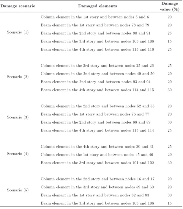
Table 3. Considered damage scenarios for plane frame under seismic loading.
Damage scenario Damaged elements Damage
value (%)
Scenario (1)
Column element in the 1st story and between nodes 5 and 6 20 Beam element in the 1st story and between nodes 78 and 79 20 Beam element in the 2nd story and between nodes 90 and 91 25 Beam element in the 3rd story and between nodes 105 and 106 15 Beam element in the 4th story and between nodes 115 and 116 25
Scenario (2)
Column element in the 3rd story and between nodes 25 and 26 25 Column element in the 2nd story and between nodes 49 and 50 20 Beam element in the 2nd story and between nodes 93 and 94 20 Beam element in the 4th story and between nodes 114 and 115 30
Scenario (3)
Column element in the 2nd story and between nodes 52 and 53 20 Beam element in the 1st story and between nodes 76 and 77 20 Beam element in the 2nd story and between nodes 88 and 89 30 Beam element in the 4th story and between nodes 115 and 114 25
Scenario (4)
Column element in the 4th story and between nodes 30 and 31 25 Column element in the 1st story and between nodes 45 and 46 20 Beam element in the 3rd story and between nodes 101 and 102 30
Scenario (5)
Column element in the 2nd story and between nodes 16 and 17 20 Column element in the 3rd story and between nodes 59 and 60 20 Beam element in the 1st story and between nodes 82 and 83 30 Beam element in the 3rd story and between nodes 105 and 106 15
6. Conclusions
In this study, an eective method based on structural deformation signal processing was introduced. In the proposed approach, the generalized S-transform was employed for identication and localization of structural damage. Due to the following reasons, the SGS-transform is a tool more powerful than wavelet
transform in time-frequency representation and signal processing:
1. The SGS-transform uses the frequency parameter
instead of the scale parameter;
2. Wavelet reconstruction leads to information
leak-age, while the SGS-transform is non-destructive and
reversible in signal reconstruction;
3. The major dierence between these two transforms is that the SGS-transform comprises the phase
factor. In other words, the SGS-transform retains
referenced phase information absolutely;
4. The SGS-transform exhibits a frequency-invariant
amplitude response in contrast to the wavelet trans-form.
To validate the eciency and applicability of the proposed method, a numerical study of damage local-ization was performed using three examples. Examples include a 3-span beam under the harmonic load, a
5-Figure 15. 55th, 57th, and 59th elements (L-1 to L-10) of the damage matrix in the beams and columns, and damage matrix spectra (R-1 to R-10) in beams and columns for all damage scenarios in Example 3.
Figure 15. 55th, 57th, and 59th elements (L-1 to L-10) of the damage matrix in the beams and columns, and damage matrix spectra (R-1 to R-10) in beams and columns for all damage scenarios in Example 3 (continued).
Figure 16. Schematic of analytical 8-DOFs system [30].
Figure 17. The Experimental 8-DOFs system with the excitation shaker attached, reproduced with kind permission from the ASME [30].
span beam under the impact load, and a 4-story 1-bay moment frame under the seismic loading. Fur-thermore, the experimental data from the vibration test of a mass-stiness system were used to verify the proposed approach. The obtained results indicated the robustness of the applied method for achieving the main objectives of damage detection in both numerical and experimental studies.
Acknowledgments
This research was supported by the Civil Engineering Department and the Research and Technology Aairs
Figure 18. (a) Damage matrix spectrum. (b) 31st, 33rd, and 35th rows of the damage matrix in the 8-DOFs system.
of Sharif University of Technology, Tehran, Iran. The authors are grateful for this support.
References
1. Amezquita-Sanchez, J.P. and Adeli, H. \Signal pro-cessing techniques for vibration-based health monitor-ing of smart structures", Archives of Computational Methods in Engineering, 23(1), pp. 1-15 (2016).
2. Doebling, S.W., Farrar, C.R., Prime, M.B., and She-vitz, D.W., Damage Identication and Health Mon-itoring of Structural and Mechanical Systems from Changes in Their Vibration Characteristics: A
Liter-ature Review, Los Alamos National Lab., NM, United States (1996).
3. Sohn, H., Farrar, C.R., Hemez, F.M., Shunk, D.D., Stinemates, D.W., Nadler, B.R., and Czarnecki, J.J., A Review of Structural Health Monitoring Literature: 1996-2001, Los Alamos National Laboratory, Los Alamos, New Mexico (2002).
4. Ditommaso, R. Mucciarelli, M., and Ponzo, F.C. \S-Transform based lter applied to the analysis of non-linear dynamic behaviour of soil and buildings", Conference Proceeding, Republic of Macedonia (2010).
5. Ditommaso, R., Parolai, S., Mucciarelli, M., Eggert, S., Sobiesiak, M., and Zschau, J. \Monitoring the response and the back-radiated energy of a building subjected to ambient vibration and impulsive action: The falkenhof tower (Potsdam, Germany) ", Bulletin of Earthquake Engineering, 8(3), pp. 705-722 (2010).
6. Gabor, D. \Theory of communication. Part 1: The analysis of information", Journal of the Institution of Electrical Engineers, 93(26), pp. 429-441 (1946).
7. Portno, M. \Time-frequency representation of digital signals and systems based on short-time Fourier anal-ysis", IEEE Transactions on Acoustics, Speech, and Signal Processing, 28(1), pp. 55-69 (1980).
8. Bloomeld, P., Fourier Analysis of Time Series: An Introduction, John Wiley & Sons (2004).
9. Cohen, L. \Time-frequency distributions-a review", Proceedings of the IEEE, 77(7), pp. 941-981 (1989).
10. Ovanesova, A. and Suarez, L. \Applications of wavelet transforms to damage detection in frame structures", Engineering Structures, 26(1), pp. 39-49 (2004).
11. Ren, W.X. and Sun, Z.S. \Structural damage identi-cation by using wavelet entropy", Engineering Struc-tures, 30(10), pp. 2840-2849 (2008).
12. Cao, M., Xu, W., Ostachowicz, W., and Su, Z. \Damage identication for beams in noisy conditions based on Teager energy operator-wavelet transform modal curvature", Journal of Sound and Vibration, 333(6), pp. 1543-1553 (2014).
13. Kaloop, M.R. and Hu, J.W. \Damage identication and performance assessment of regular and irregular buildings using wavelet transform energy", Advances in Materials Science and Engineering, 2016, pp. 1-11, Article ID: 6027812, Hindawi (2016).
14. Janeliukstis, R., Rucevskis, S., Akishin, P., and Chate, A. \Wavelet transform based damage detection in a plate structure", Procedia Engineering, 161, pp. 127-132 (2016).
15. Balafas, K., Kiremidjian, A.S., and Rajagopal, R. \The wavelet transform as a Gaussian process for damage detection", Structural Control and Health Monitoring, 25(2), pp. 1-20 (2017).
16. Stockwell, R. \Why use the S-transform. AMS pseudo-dierential operators: Partial pseudo-dierential equations and time-frequency analysis", Fields Institute Commu-nications, 52, pp. 279-309 (2007).
17. Stockwell, R., Mansinha, L., and Lowe, R. \Localiza-tion of the complex spectrum: the S transform", IEEE Transactions on Signal Processing, 44(4), pp. 998-1001 (1996).
18. Bindi, D., Parolai, S., Cara, F., Di Giulio, G., Ferretti, G., Luzi, L., Monachesi, G., Pacor, F., and Rovelli, A. \Site amplications observed in the Gubbio basin, cen-tral Italy: hints for lateral propagation eects", Bul-letin of the Seismological Society of America, 99(2A), pp. 741-760 (2009).
19. Parolai, S. \Denoising of seismograms using the S-transform", Bulletin of the Seismological Society of America, 99(1), pp. 226-234 (2009).
20. Pakrashi, V. and Ghosh, B. \Application of S-transform in structural health monitoring", 7th In-ternational Symposium on Nondestructive Testing in Civil Engineering (NDTCE), Nantes, France (2009).
21. Ditommaso, R., Mucciarelli, M., Parolai, S., and Pi-cozzi, M. \Monitoring the structural dynamic response of a masonry tower: Comparing classical and time-frequency analyses", Bulletin of Earthquake Engineer-ing, 10(4), pp. 1221-1235 (2012).
22. Ditommaso, R., Mucciarelli, M., and Ponzo, F.C. \Analysis of non-stationary structural systems by using a band-variable lter", Bulletin of Earthquake Engineering, 10(3), pp. 895-911 (2012).
23. Ditommaso, R., Ponzo, F., and Auletta, G. \Dam-age detection on framed structures: modal curvature evaluation using Stockwell transform under seismic excitation", Earthquake Engineering and Engineering Vibration, 14(2), pp. 265-274 (2015).
24. Addison, P.S., The Illustrated Wavelet Transform Handbook: Introductory Theory and Applications in Science, Engineering, Medicine and Finance, CRC Press (2017).
25. Mallat, S., A Wavelet Tour of Signal Processing, San Diego, Academic Press (1999).
26. Stockwell, R. \A basis for ecient representation of the S-transform", Digital Signal Processing, 17(1), pp. 371-393 (2007).
27. Pinnegar, C. and Mansinha, L. \Time-local Fourier analysis with a scalable, phase-modulated analyzing function: The S-transform with a complex window", Signal Processing, 84(7), pp. 1167-1176 (2004).
28. Wang, Y., The Tutorial: S-Transform, Graduate Insti-tute of Communication Engineering, National Taiwan University, Taipei (2010).
29. Alwash, M., Sparling, B.F., and Wegner, L.D. \Inu-ence of excitation on dynamic system identication for a multi-span reinforced concrete bridge", Advances in Civil Engineering, 2009, pp. 1-18, Article ID: 859217, Hindawi (2009).
30. Duey, T.A., Doebling, S.W., Farrar, C.R., Baker, W.E., and Rhee, W.H. \Vibration-based damage iden-tication in structures exhibiting axial and torsional response", Journal of Vibration and Acoustics, 123(1), pp. 84-91 (2001).
Biographies
Hamed Amini Tehrani received his BSc and MSc degrees in Civil Engineering from Iran University of Science and Technology. He is currently a PhD candi-date at the Sharif University of Technology, Iran. His research interests include structural health monitoring, structural system identication, signal processing, and random vibrations in earthquake engineering.
Ali Bakhshi earned his BSc and MSc degrees in Civil and Structural Engineering from Sharif University of Technology (SUT) and Shiraz University in 1988 and
1990, respectively. In 1998, he received his PhD from Hiroshima University, Japan, where he joined as a faculty member in the same year. In 2000, he moved to SUT, where he is currently an Associate Professor. He is actively involved in design and installation of shaking table facility; since then, he contributed in many experimental testing types of research. Dr. Bakhshi's main interests include experimental and analytical research in structural control, seismic performance of adobe structures, seismic hazard and risk analyses, and random vibrations. He has published many papers in international journals and conferences.
Moustafa Akhavat received a BSc degree in Civil Engineering from Azad University of Arak, Iran, and an MSc degree in Earthquake Engineering from Iran University of Science and Technology. His research interests include soil-structure interaction, earthquake engineering, and structural health monitoring.