David P. Miller.
An Exploratory Study of Using NoSQL Databases to Store Weather
Data
.
A Master’s Paper for the M.S. in I.S degree
.
March,
2012
.
33
pages.
Advisor: Arcot
Rajasekar
Current weather observations are not sufficient spatially or temporally to resolve all
weather phenomena, but a large increase in the data intake would cause new problems
with storage. NoSQL databases are potential solutions that offer fast queries and the
ability to scale to incredibly large sizes. This study examines some of the unique
characteristics of weather data and if they can be leveraged in a NoSQL environment.
Data models were designed and tested for two NoSQL databases, Cassandra and Hbase,
to see if they can meet all of the necessary query functionality and a few basic speed tests
were run to gauge baseline query speeds.
Headings:
Database Design
by
David P. Miller
A Master’s paper submitted to the faculty
of the School of Information and Library Science
of the University of North Carolina at Chapel Hill
in partial fulfillment of the requirements
for the degree of Master of Science in
Information
Science
.
Chapel Hill, North Carolina
March 2012
Approved by
1. Introduction
Recent research that looked at data taken from commercial aircraft revealed that the intensity of the jet stream can vary significantly and frequently (Cardinali 1870-1). Currently the European Centre for Medium-Range Weather Forecasts (ECMWF) takes aircraft data into their model to help resolve upper atmosphere wind and temperature patterns. The data is thinned so that readings are spaced at least 60 kilometers apart, but with this data resolution the detailed structure of the jet stream can be lost. This study looked at a finer granularity of readings and noticed that the velocity readings of aircraft flying though the jet stream showed frequent peaks, possibly due to embedded gravity waves. These features only showed up in high frequency data and the ECMWF have said that underestimation of analyzed jet streaks is a common problem in their model.
Current weather prediction is not the only area that could benefit from an influx of new data. Climate change is one of the most hotly debated topics in politics and weather circles. There is a wealth of historical weather data stored in log books of ships that goes back to the 1600’s and covers many areas that have very little coverage otherwise (Brohan 220).
Historically there has been a scarcity of readings from over oceans, and the United Kingdom has hundreds of thousands of log books from the Royal Navy and the Honorable East India Company that cover areas from Greenland around the horn of Africa and into the Indian Ocean. With the addition of all this data we could form a much clearer picture of how our climate has changed from well before the Industrial Revolution up through current times.
for the past 30 years and excel at storing and retrieving highly structured data like weather data. The drawback of relational databases is that they do not scale well with large scale data, so another solution is needed for a problem of this size. In the last decade NoSQL databases have risen to popularity because they scale incredibly well and can handle the kinds of unstructured data that is commonly found on the web (Han). NoSQL databases serve as the backend for many of the internet’s largest operations, such as Google’s search interface and Amazon’s online store (Decandia, Chang). This research will look into the combination of weather data and NoSQL databases to see if NoSQL databases can provide all of the needed functionality and if the structured nature of weather data can be leveraged for performance gains. Two NoSQL databases will be examined, Cassandra and Hbase. Both will be loaded with the same data and then a series of tests will be run to determine the usability of the query functionality and the performance of each database.
The following sections of this thesis will give a brief overview of important database concepts in both relational and NoSQL database systems, analyze the unique properties of weather data, present a few brief case studies of NoSQL system implementations and compare and contrast them to a weather implementation, outline the experiment that was run, and discuss the results obtained.
2. Database Overview
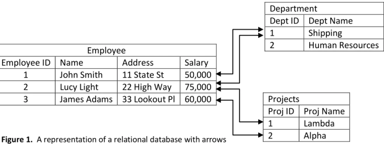
into one table based on its functional relationships and as needed the tables are related to each other so that all of the many-to-one and many-to-many mappings are retained. The classic example of this is a database for a company that contains employees, departments, and projects (Figure 1). Each row in the employee table contains a variety of information for that employee such as name, address and salary which are highly related. Relations are then inserted to point each employee to the departments they work for and the projects they are working on. The exact nature of these mappings is dictated by the structure of the information space; if an employee can only be a part of one department then employee -> department will be a one-to-many relationship. Relational databases tend to have tables that are densely packed since one of the objectives in the design is to eliminate redundant information and missing values. Furthermore, if there are changes to the structure of the database at a later date it can create considerable problems since large parts of the design and query structures may have to be reworked.
Figure 1. A representation of a relational database with arrows
representing the relations. Tables are densely packed with few missing values or repeated information.
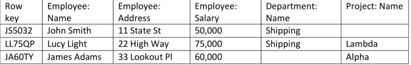
NoSQL databases do not split information into many small tables but instead keep all of the information in one large, sparsely populated table (Figure 2). Each row still contains
information about a single employee, but instead of separating out the department and project Department
Dept ID Dept Name 1 Shipping
2 Human Resources Employee
Employee ID Name Address Salary 1 John Smith 11 State St 50,000 2 Lucy Light 22 High Way 75,000
3 James Adams 33 Lookout Pl 60,000 Projects
Proj ID Proj Name
1 Lambda
information it is attached in separate columns to each employee. Since there are no relations present then NoSQL databases can store the information based on columns instead of storing based on rows like a traditional relational database. Both Cassandra and Hbase allow columns to be grouped into families to further control what kinds of data are stored together. For example, the database could be storing both numerical readings from an observation, which are small and quick to retrieve, and radar images which can be very large and slow to retrieve. It would take a careful design to separate both kinds of data in a relational database to ensure that queries of the numerical data were not slowed down by the radar images. In a NoSQL system both radar images and numerical data would only need to be tagged with different column families to ensure that they are stored efficiently.
This approach does lead to a lot of redundant information being stored in the database. Furthermore, when new information needs to be inserted into the database structure it only requires the creation of a few new columns and not a large reworking. That is not to say that there is no work put into the design of the data model for a NoSQL system, the design of the tables and creation of row keys has to be tailored to how the information will be queried instead of any inherent structure to the data. This can frequently lead to the same data being stored in multiple tables just to facilitate faster queries.
Row key
Employee: Name
Employee: Address
Employee: Salary
Department: Name
Project: Name JS5032 John Smith 11 State St 50,000 Shipping
LL75QP Lucy Light 22 High Way 75,000 Shipping Lambda
JA60TY James Adams 33 Lookout Pl 60,000 Alpha
One main concept that is essential to both relational and NoSQL databases is the
primary key. The primary key is the piece of information that allows us to uniquely identify each row in the table. There are a couple of important concepts that define all primary keys,
uniqueness and permanence. The key needs to be unique so that a query will only find the relevant information and permanent so that if aspects of your data change over time it will not be split and stored in separate places. If we look back at the employee example, what would make a good primary key for an employee? The first natural reaction may be the employee’s name since it is what we use everyday to differentiate people from one another. But looking closer we realize that both concepts behind the primary key are violated when using a name. First, names are not unique. Even in very small companies it is possible for two employees to have the same name so something else would be needed to differentiate them. Second, names are not permanent. It is very common and even expected that when two people get married that one of them takes the other’s name. From a database perspective this would lead to one employee having multiple collections of records that are not connected. Another solution might be to use a person’s Social Security Number as a primary key since it should be unique.
Unfortunately, not all Social Security Numbers are unique, they are changed in some cases, and not everyone in the United States has a Social Security Number, so selecting a good primary key takes a lot of forethought and effort.
2.1 Hbase
Hbase is an open source NoSQL database that is based on Google’s BigTable. While Hbase can be run on a single machine, it is designed to have multiple machines each performing specific roles to facilitate faster query speeds (Architecture). There are three main roles, master server, lock server, and region server. A single master server, which may be replicated, oversees the entire operation, ensuring that everything runs smoothly and any machine failures are dealt with quickly. A single lock server, possibly replicated, maintains locks on the region servers so that only authorized access to the data is allowed. Multiple region servers house the actual data, since all of the data is stored in one or more large tables it is split up into chunks and each regions server gets a piece. The data in the table is stored in lexicographic order by the primary key, typically called a row key (Row Key Design). Smart row key design becomes especially important so that similar data is stored together which should improve query performance. One thing needs to be noted, however. Since Hbase stores everything in bytes there can be some unexpected behavior with numerical row keys which will be used for weather data. Negative numbers appear first in lexicographic order, but for simplicity we will avoid this problem by using positive values for row keys. Second, decimal numbers will need to be padded with zeros to ensure that all row keys are a constant sized string.
2.2 Cassandra
allow the storage of columns inside of columns. This leads to some interesting possibilities with weather data which will be expanded upon later. From a hardware perspective, Cassandra is very different from Hbase. Every machine in a Cassandra system is a built to stand on its own; there are no specific roles for different machines. This allows a Cassandra system to be spread over a much larger geographical distance since the communication time between different clusters of machines is not critical. Data is stored by the hash of the row key; each machine is assigned a range of hashes and any new data that falls in that range is stored on that machine (About Data Partitioning in Cassandra). Individual machines in a cluster are arranged in a ring so that their hash ranges line up sequentially. Cassandra employs a quorum that allows the
administrator to determine how many sequential machines will store backups of data. Clients can make queries to any machine in a Cassandra cluster (About Client Requests in Cassandra). When the query is received it will be sent to all of the machines that have copies of the relevant data and when a sufficient number of responses, which can also be set by the administrator, have been received the response is sent back to the client. Since there is no master server in a Cassandra cluster all machines use a gossip protocol to determine the destination for queries and deal with machine failures (About Internode Communications (Gossip)). All machines operate on a heartbeat and every beat each machine sends a list of its hashes to different random machine in their ring. This way all machines have an index of the hashes of all other machines and can route queries effectively. When one machine fails it takes only takes a few beats for enough other machines to realize the failure and redistribute the data load to account for it.
As mentioned before, one of the main differences between relational databases and NoSQL databases is that NoSQL databases excel at storing unstructured data. Think for a moment of Amazon’s online store, which is supported by another NoSQL database, Dynamo. Each row in the database could pertain to a different product offered on Amazon.com and store information like the price, quantity and a picture. There would be millions of these products, and while they could be grouped into categories like books and shirts, we would not be able to infer any information about one product from looking at another product. Unstructured data like this can be thought of as a collection of unrelated items, and the main challenge is finding the correct item and returning the relevant information. Weather data is different. The collection of items in weather data, let’s say weather stations, are closely related. We would expect that two weather stations that are separated by a short distance to report similar readings. In the event that the readings differed greatly, there is significance in that as well. It could indicate the presence of a strong weather front moving through or that one of the stations is malfunctioning in some way. It is very difficult to make the same kinds of inferences from a collection of items on Amazon.com.
three aspects to be useful, the time of the occurrence, the location of the occurrence, and what actually occurred. A combination of time and location would also make a good candidate for a row key since it neatly divides weather data into a set of instances, but as with any row key design a closer examination is required to anticipate any unique quirks that could arise.
Currently location is encoded in a station identifier which is sent along with the observation. In the United States we typically use the International Civil Aviation Organization (ICAO) airport codes, such as KRDU or KIAD, but there are many different encoding standards worldwide so this can vary depending on the data set being viewed. Another drawback to using a station identifier is that, on its own, it tells us nothing about where the station is located. There would still need to be a separate index that tracked the exact coordinates of each station. In addition, some stations are expected to move, such as the weather instruments that are attached to commercial aircraft. Simply tracking this data by the flight number would lose an essential dimension to the data. Instead of adding an extra level of data that needs to be tracked it would be easier to just track all observations by the Geographic Information System (GIS) coordinates of the station. Each reading could still be tagged with the kind of station that recorded it in case the instrumentation has differing levels of accuracy. GIS also includes an altitude component in addition to latitude and longitude readings which would be very useful from a meteorological standpoint.
taken. From a database perspective, these movements could cause the readings for one station to be stored in different parts of the table and a simple query for a station’s GIS coordinates would not return all of the data. In order to access all of the data for one station we would need to search by all of the coordinates that the station had ever occupied. Fortunately, one of the other basic requirements can be used to bypass this problem. As mentioned before range queries are going to be important for weather data, so in order to get all of the data for a specific station it would only be necessary to do a very small range query around a single point. Queries that encompassed a larger area would naturally pull all readings for the individual stations already. So even though the permanence aspect of the primary key is not satisfied location is still a valuable aspect of uniquely identifying individual observations.
Comparatively, time is a much more straight forward element. The only potential issues could arise with the format that time is stored in. A lot of databases store time formats in something similar to ‘number of seconds since’ an arbitrary date. For Linux systems this is January 1st, 1970. This would cause problems storing data from before 1970; if it was given a negative time then the lexicographic order would sort these times backwards. It is much easier, and makes more sense, to store dates in a simple string format similar to YYYYMMDDhhmmss (Year, Month, Day, hour, minute, second). Problems can arise with data that is taken on different time scales, such as daily or monthly averages. Rather than standardizing the hours and minutes to some arbitrary time, like midnight, these readings should be put in separate tables that only encode time down to the day or month.
could end up being stored on the same server. This would overload one particular machine while others were underutilized. Conversely, by storing location – time all data would be first grouped by geographic location and then by time, so new data coming in would be scattered throughout the table and theoretically would be balanced throughout all of the machines. Storing data by location – time would mean that queries that pull a series of data from one station would be faster than queries that pulled data over a wide range of stations at one point in time. Queries that pulled data from a range of stations at multiple times would not be faster either way.
Throughout all of this discussion one specific query has been ignored, returning the current conditions. Since this query would be performed very frequently it makes sense to optimize for it by storing current conditions in their own table. This table would only use the location as a row key so that when new readings came in they would simply overwrite the old readings at that same location and only the most current data would be stored in this table. Time would still need to be tracked as a column to perform cleanup on stations that do move locations. In the event of a station moving, the last data point at the old location would never be overwritten, so having the time stored would allow us to delete these readings after a certain time frame.
4. Use Cases
As previously mentioned, NoSQL database implementations depend largely on the kinds of data being stored and how it will be queried. Before we get into the specific data models that are used, let’s examine a few real world implementations that chose between Hbase and
Mozilla, the company that makes the Firefox web browser, has a project called Mozilla Labs Test Pilot that collects data from users to help designers create a better user experience (Deinspanjer). They are very open and up front about their data collection tactics and make sure that the user’s privacy is ensured. As the project moved out of the early stages they anticipated increasing their user numbers to tens of millions, collecting over one terabyte of data, and having the majority of their data collection occurring in two short windows of time. This means that their system would need to perform well under peak load and not simply sit idle during downtime. They looked at three NoSQL databases, Hbase, Cassandra, and Riak, and while they ultimately chose Riak mostly for a lower up front cost and less software development to get started, they did make some interesting comments about the utility of both Hbase and Cassandra. One of the main points against both was that a hand made front end would be necessary since both databases do very few security checks like checking payload size and inspecting data for missing or incomplete values. This would also be essential in a weather implementation. One of the major differences between Hbase and Cassandra was that on Hbase some types of administration and upgrades still required a restart of the entire cluster which creates a maintenance window when the service is not available. All of Cassandra’s maintenance only required rolling restarts. This would be especially useful in a weather implementation since there would never be a time when the system is not taking in data, so even a small amount of maintenance would require an alternate way to ensure data is not lost.
Netflix is another company that has moved a number of its services to the cloud and is reliant on NoSQL databases to support them (Izrailevsky). In a blog post last year Yury
while also running MapReduce jobs. As for Cassandra, Netflix was impressed with the ability to split its clusters across the United States to give equal service to different geographical regions. They also made use of the ability to configure the consistency and replication models to the job being performed. Being able to split clusters up geographically could be very useful for a
weather implementation. If local readings were stored on a local cluster it would allow writes to process quickly but could slow down reads in some situations. If the majority of people
requested a nationwide view of the weather then the system would have to routinely request information from multiple clusters.
In early 2010, Dominic Williams wrote a blog post about how a small company that he was working for was designing a massively multiplayer online game and had just finished the process of converting their back end from Hbase to Cassandra (Williams). He was obviously very positive on Cassandra, citing the flexibility of the quorum, the ease of setup, and low
maintenance and tuning. But the most interesting point was how he differentiated the two databases. He says, “Hbase [is] more suitable for data warehousing, and large scale data processing and analysis” which would seem to describe a weather implementation. He goes on to describe Cassandra as “being more suitable for real time transaction processing and the serving of interactive data”. This also describes essential functions to a weather system with real time transaction processing for the new data coming in and the interface serving the interactive data. It is possible that a weather system would be best served by a combination of both systems, and this is a common problem in NoSQL databases. Most NoSQL systems were designed to solve a specific problem that current systems were just not good enough for.
made may still apply. This is some of the most recent information available but NoSQL databases are evolving quickly with new features being released a few times a year.
5. Data Models
5.1 Hbase
The data model for Hbase is fairly straight forward. Without all of the enhancements that Cassandra offers there is not much flexibility to experiment with. Row keys will be a combination of location – time and columns will contain the various parameters to be tracked. In order to maximize query speed columns should be grouped into families based on data types, where numerical readings are separated from larger data types like images. Finer grained column groupings are acceptable, as long as they do not group dissimilar data types together.
One problem that could not be solved through manipulating the data model was being able to run a query that returned data from multiple stations over a period of time. While Hbase does allow range queries, it only allows them on the row key and only allows one range per query. The previously mentioned query would take multiple ranges on various fields, such as a range on latitude, longitude, and time. Since a typical row key would be stored as latitude, longitude, altitude – time, then stations that had the same latitude would be stored next to one another even if they were on opposite sides of the Earth. Even switching around the order of the parameters would not avoid this problem. What is needed is the ability to create
geographic boxes where a small range is taken from a few different parameters.
extremely large jobs that can take hours to run and use hundreds of machines; the setup process alone can take over a minute, and is usually fairly resource intensive (How Many Maps?). Using MapReduce for such a common query would overtax the system and taking over a minute to return a simple query is simply too long.
5.2 Cassandra
While the data model for Cassandra can be tweaked to resemble Hbase’s exactly, there were many more options to experiment with to see if a better solution could be devised. Cassandra gives users a choice on how to partition the data that is read into the table. The Order Preserving Partitioner (OPP) mimics Hbase where row keys are stored in order and allows Cassandra to use range queries on the row key. The Random Partitioner (RP) stores row keys by their MD5 hash which will automatically scatter them across different machines, and makes range queries on the row key essentially useless. While the OPP seems to give more functionality, it does run the risk of overloading certain machines and would make the load balancing something that needs to be watched carefully by the database administrator. However, due to the structured nature of weather data it may be easier to anticipate server load since we can anticipate what future row keys will resemble. Most documentation and use cases that were looked at strongly encourage the use of the RP and since other features made range scans on row keys redundant, the Random Partitioner should be used.
column, however. Rows are essentially limitless; Cassandra is designed to expand to infinity in the row dimension. The parent column can hold up to two billion values, but the child column is not recommended to have more than a handful of values (JohnathanEllis). Assuming that time would be mapped into rows since both would keep expanding infinitely, there is not a good match for the remaining two categories. Both location and parameters would easily expand beyond a handful of values so the child column is not useful, and even the parent column could have trouble holding all of the values for location depending on how precise the readings for the GIS coordinates are.
One other concept that has not been explained previously is the timestamp. When a piece of data is stored, the time of insertion is also stored with it. The timestamp is mostly used to resolve write conflicts and for garbage collection, but it is accessible in the data model. One early experiment looked at using the timestamp to store the time dimension, but similar to the child column it is only designed to hold a small number of values and was too important in the underlying features of Cassandra to be manipulated. This idea was quickly discarded.
every day at a station where the temperature got above 60 degrees, but how often is this query really going to be run? These questions will be difficult to answer without knowing who the users are and how the system will be used. If the system is simply a data repository that allows users to download large chunks of historical data, then a lot of the analysis can be done in separate programs. However, if the system is designed to do the analysis itself then these types of queries may be necessary.
The final data model is similar to Hbase’s where all rows are stored with row keys using location – time format. Parameters will be stored in columns, with similar data types being grouped together in column families and further refinements as necessary. In addition, latitude, longitude, altitude and the time will also be stored in indexed columns to facilitate querying. The system will use the random partitioner and no super columns. Additional tables will be created as necessary for data that is stored on different time frames, such as daily and monthly averages, and for the current conditions as explained earlier.
6. Experiment
There were two main goals to this research: to explore whether or not weather data could be effectively stored in a NoSQL database and to run some preliminary speed tests to determine if there were major differences between Hbase and Cassandra. The preceding sections of this paper have addressed the first goal and the remaining sections will outline the experiment that was run for the second goal.
6.1 Data
http://www.waterbase.org/download_data.html but is also available from the NCDC directly at http://www7.ncdc.noaa.gov/CDO/cdoselect.cmd?datasetabbv=GSOD&countryabbv=&georegio
nabbv=. The data consisted of a daily average of many of the fields that are reported in a standard NWS observation. For a more detailed look at the specific fields that were used and the data cleaning efforts that were undertaken, see Appendix A.
6.2 System
All experiments were performed on one machine that ran both instances of Hbase and Cassandra. The tests were done on the most current versions of Hbase and Cassandra at the start of the experiment; Hbase version 0.90.4 and Cassandra version 0.80. The machine had an Intel Pentium 4 3.6 GHZ processor, 3 GB of RAM, 450 GB hard drive, and running Ubuntu 10.04. The machine was accessed from an offsite location using a Secure Shell Client. To create tables and insert data a combination of command line interface and Python based client were used. For Hbase all tables and keyspaces were created with the Hbase shell and all data insertion was done through a Jython connection. For Cassandra, all tables and keyspaces were created through the Cassandra CLI and data insertion was done with Pycassa, a Python based connection.
6.3 Tests
observations and over 10,000,000 data values. For the one station test, queries were run through the Hbase shell and Cassandra CLI to access data from 10 different stations over
increasing periods of time. Each individual query was run twice and averaged. The geographical area test accessed data from a small area around the same stations as the single station test and over the same time periods. Each area was large enough to take in more readings than the single station test. The geographical area test was only run once per area and only on Cassandra since Hbase could not process these complex queries. All query speeds were measured with the Hbase shell and Cassandra CLI, the insertion speeds were measured in wall clock time.
6.4 Results and Discussion
The insertion test results were surprising; Cassandra handed all 420,000 observations in around 22 minutes while Hbase took nearly 14 hours to insert the January 2000 data and after a few tweaks February 2000 was inserted in around 11 hours. While Cassandra is optimized for write operations and it was expected that Cassandra would outperform Hbase, the results were extremely lopsided. I suspect there are two culprits for this result. First, Hbase required that each piece of information be inserted separately. For Cassandra one procedure call could be used to insert all 25 pieces of information for an individual observation, while Hbase required that each individual piece of information be added separately so it took 25 procedure calls to insert one observation. Secondly, there was no log displayed for Cassandra as write operations preceded, while for Hbase every addition created a log that was displayed to the screen. This could have been a feature of the Jython connection that was being used, but it is suspected that the second issue was a bigger contributor to Hbase’s poor performance.
increased. This accounts for most of the performance increase between the two months, although February did have about 10,000 less observations than January. Additionally, for the Hbase data there are two distinct phases, preparation and insertion. The preparation of the data involves adding each individual parameter to an array, and then the insertion takes that array and writes it to the database. One alternative that was explored to improve performance was to create a multi-dimensional array of 10,000 observations and then measure the insertion time. This alternative was designed to isolate whether the preparation or the insertion was slowing down the write speed. The multi-dimensional array took around 45 minutes to create and under 15 seconds to insert. Clearly the preparation of the data was reason for the slow write speeds, but unfortunately I did not have the knowledge to correct it. Hbase does not seem to be designed to add multiple pieces of data at once, and I could not find any options to turn off the logging mechanism that was slowing down the preparation of the data.
In the one station query test Cassandra routinely outperformed Hbase by returning the results roughly twice as fast for every query. Both databases saw performance slow slightly as
0 0.05 0.1 0.15 0.2 0.25 0.3 0.35 0.4 0.45
1 2 3 4 5 6 7 8 9 10
T im e (s ) Test Number
Test # 2: Data from One Station Over a Period of Time
more readings were accessed. Both databases performed within reasonable expectations and it is expected these speeds could be improved with in a larger implementation.
The geographic area test saw a significant decrease in performance in Cassandra
regardless of how many results were returned. While it is notable that Cassandra could perform these queries, taking over three minutes to return a set of results would not be acceptable in any implementation. Originally the CLI was set to time out after 10 seconds on queries and that limit had to be raised twice before a query would complete.
The degradation in performance is mostly due to how Cassandra handles queries of this type. Each query must contain at least one equality (‘=’) operation in order to execute any greater than/ less than (‘><’) operations. Cassandra then scans through the table creating a list of all records that match the equality operations and filters those results based on the greater than/less than operations. No part of the geographic area query could satisfy the equality requirement so a dummy variable was inserted into each observation that was set to ‘yes’.
0 100 200 300 400 500 600
1 2 3 4 5 6 7 8 9 10
Test Number
Test #3: Cassandra - Data from a Geographic Area Over a
Period of Time
Time (s)
Queries used the dummy variable for equality and attached six greater than/less than operations, one set for latitude, longitude, and time. The altitude dimension was ignored for simplicity and since a data set this small had no conflicts where the altitude was essential. The end result was that Cassandra scanned the entire table to create a list of all the records which was then filtered down based on the area and time constraints. This problem would only be compounded in a larger implementation. The data will need to be broken down into smaller chunks that are stored in separate tables, either geographically by country or temporally by month or day. Another option is to improve how Cassandra handles secondary indexes; they were recently added to Cassandra and will most likely be improved in forthcoming versions.
7. Limitations
There are a couple of major limitations to the speed tests performed in this experiment. First, I did not have access to the kinds of equipment to properly set up a full scale
implementation of either Cassandra or Hbase. Both of these databases are designed to run on multiple machines that are each more powerful than the one machine that I did have.
8. Conclusion
Appendix A: Data Fields and Cleaning
The data for this experiment consisted of 23 fields: 1-Station Number
2-WBAN number 3-Year
4-Month and Day 5-Temperature 6-Temperature Count 7-Dewpoint
8-Dewpoint Count 9-Sea Level Pressure
10-Sea Level Pressure Count 11-Station Pressure
12-Station Pressure Count 13-Visibility
23-Indicators for Fog, Rain, Snow, Hail, Thunder, Tornado
For fields 5 – 16 the first value of the pair is the average for the day and the second value is the number of readings that went into the average. Fields 19, 20, and 21 could also have additional flags attached to them to give more information about how the reading was taken, but for this experiment any extra characters were just included with the reading. WBAN numbers were not stored in the database, and fields 3 and 4 were concatenated to create one field that contained the year month and day. In addition, a dummy variable was created to allow Cassandra to perform the geographic area queries.
A separate list of the latitude, longitude, and altitude of each station was also provided and these coordinates were used in the row key for each reading. All longitude and altitude values were already padded with zeros, but latitude needed one extra zero added to account for the conversion of negative numbers. To deal with negative values the following steps were taken. For negative longitude values, the value was added to 360. This created a natural range of values from 0 to 360 that would logically progress from the Prime Meridian eastward around the globe. For negative latitude values, the value was added to 360. This puts northern
latitudes at their natural 0 to 90 ranges but converts southern latitudes to a range between 270 and 360. There are no readings between 90 and 270. Both latitude and longitude are stored with their correct negative values in the individual columns. For negative altitudes, the absolute value of the reading was stored. This does leave a potential conflict open where two stations could have the same latitude and longitude and positive/negative altitudes, possibly due to a ground station and low flying aircraft. This data set did not have such a conflict but a real world implementation would need a more elegant solution even though negative altitudes should be relatively small (under 50 meters) and infrequent.
Row key-LatitudeLongitudeAltitude-YearMonthDay 1-Station Number
2-Latitude 3-Longitude 4-Altitude 5-YearMonthDay 6-Temperature 7-Temperature Count 8-Dewpoint
9-Dewpoint Count 10-Sea Level Pressure 11-Sea Level Pressure Count 12-Station Pressure
13-Station Pressure Count 14-Visibility
Appendix B: Sample Queries
Test #2: Single station Hbase:
scan 'weather', {STARTROW => '3528136250040-20000101', STOPROW => '3528136250040-20000103'}
scan 'weather', {STARTROW => '3621001330144-20000104', STOPROW => '3621001330144-20000109'}
Cassandra:
get WeatherData where StationNumber = 477610 and YearMoDa > 20000100 and YearMoDa < 20000103;
get WeatherData where StationNumber = 604250 and YearMoDa > 20000103 and YearMoDa < 20000109;
Test #3: Geographic Area
Cassandra:
get WeatherData where Dummy = 'Yes' and Lat > 3500 and Lat < 3600 and Long > 13600 and Long < 13750 and YearMoDa > 20000100 and YearMoDa < 20000103 limit 200;
References
“About Client Requests in Cassandra.” Apache Cassandra 1.0 Documentation. Apache Software Foundation. n.d. Online. 27 March 2012.
“About Data Partitioning in Cassandra.” Apache Cassandra 1.0 Documentation. Apache Software Foundation. n.d. Online. 27 March 2012.
“About Internode Communications (Gossip).” Apache Cassandra 1.0 Documentation. Apache Software Foundation. n.d. Online. 27 March 2012.
“Architecture.” Apache Hbase Reference Guide. Apache Software Foundation. 2 March 2012. Online. 27 March 2012.
“Automated Surface Observing Systems (ASOS).” srh.noaa.gov. National Weather Service. 5 January 2010. Online. 15 March 2012.
Brohan, Philip, Rob Allan, J. Eric Freeman, Anne M. Waple, Dennis Wheeler, Clive Wilkinson, and Scott Woodruff. “Marine Observations of Old Weather” Bulletin of the American Meteorological Society. 90.2 (2009): 219-230. Print.
Cardinali, Carla, Lars Isaksen, and Erik Andersson. “Use and Impact of Automated Aircraft Data in a Global 4DVAR Data Assimilation System” Monthly Weather Review 131.8 (2003): 1865-1877. Print.
Chang, Fay, Jefferey Dean, Sanjay Ghemawat, Wilson C. Hsieh, Deborah A. Wallach, Mike Burrows, Tushar Chandra, Andrew Fikes, Robert E. Gruber. “Bigtable: A Distributed Storage System for Structured Data.” ACM Transactions on Computer Systems 26.2 (2008): 1-26. Print.
“Deadliest Earthquakes.” NOVA. PBS. 2012. Online.
Decandia, Giuseppe, Deniz Hastorun, Madan Jampani, Gunavardhan Kakulapati, Avinash Lakshman, Alex Pilchin, Swaminathan Sivasubramanian, Peter Vosshall, Werner Vogels. “Dynamo: Amazon’s Highly Available Key-Value Store.” 21st ACM Symposium on
Operating System Principles, Stevenson, WA, October 14-17 2007. Print.
Han, Jing, E. Haihong, Guan Le, Jian Du. "Survey on NoSQL database" Pervasive Computing and
Applications (ICPCA), 2011 6th International Conference 26-28 Oct. 2011, 19 December
2011. Print.
“How Many Maps?” MapReduce Tutorial. The Apache Software Foundation. 14 February 2012. Online. 15 March 2012.
Izrailevsky, Yuri. “NoSQL at Netflix” The Netflix Tech Blog Netflix 28 January 2011. Online. 28 February 2012.
JohnathanEllis “Cassandra Limitations.” Cassandra Wiki. n.p. 16 February 2012. Online. 28 February 2012.
“Overview.” MapReduce Tutorial. The Apache Software Foundation. 14 February 2012. Online. 15 March 2012.
“Row Key Design.” Apache Hbase Reference Guide. Apache Software Foundation. 2 March 2012. Online. 27 March 2012.
“Surface Weather Observation Stations.” FAA.gov. Federal Aviation Administration. 27 December 2010. Online. 15 March 2012.
“What is the Coop Program?” nws.noaa.gov. National Weather Service. 14 September 2009. Online. 15 March 2012.