JOINT TRANSPORTATION
RESEARCH PROGRAM
INDIANA DEPARTMENT OF TRANSPORTATION AND PURDUE UNIVERSITY
Implementation of Weigh-in-Motion
Data Quality Control and
Real-Time Dashboard Development
Wayne A. Bunnell, Howell Li, Michael Reed, Timothy Wells,
Dwayne Harris, Marc Antich, Steven Harney, Darcy M. Bullock
RECOMMENDED CITATION
Bunnell, W. A., Li, H., Reed, M., Wells, T., Harris, D., Antich, M., Harney, S., & Bullock, D. M. (2018).
Implementation of
weigh-in-motion data quality control and real-time dashboard development
(Joint Transportation Research Program
Publica-tion No. FHWA/IN/JTRP-2018/11). West Lafayette, IN: Purdue University. https://doi.org/10.5703/1288284316731
AUTHORS
Wayne A. Bunnell
Field Implementation Research Engineer
Lyles School of Civil Engineering
Purdue University
Howell Li
JTRP Senior Software Engineer
Lyles School of Civil Engineering
Purdue University
Timothy Wells
Section Manager
Indiana Department of Transportation
Dwayne Harris, PhD, PE
Transportation Research Engineer
Division of Research and Development
Indiana Department of Transportation
JOINT TRANSPORTATION RESEARCH PROGRAM
Marc Antich
LAN Administrator
Traffic Management Division
Indiana Department of Transportation
Steven Harney
Traffic Management Planning Specialist
T
raffic Management Center
Indiana Department of Transportation
Darcy M. Bullock, PhD, PE
Lyles Family Professor of Civil Engineering
Lyles School of Civil Engineering
Purdue University
(765) 494-2226
[email protected]
Corresponding Author
The Joint Transportation Research Program serves as a vehicle for INDOT collaboration with higher education
in-stitutions and industry in Indiana to facilitate innovation that results in continuous improvement in the planning,
design, construction, operation, management and economic efficiency of the Indiana transportation infrastructure.
https://engineering.purdue.edu/JTRP/index_html
Published reports of the Joint Transportation Research Program are available at http://docs.lib.purdue.edu/jtrp/.
NOTICE
The contents of this report reflect the views of the authors, who are responsible for the facts and the accuracy of the
data presented herein. The contents do not necessarily reflect the official views and policies of the Indiana Depart
-ment of Transportation or the Federal Highway Administration. The report does not constitute a standard, specifica
-tion or regula-tion.
COPYRIGHT
Copyright 2018 by Purdue University. All rights reserved.
Print ISBN: 978-1-62260-503-3
TECHNICAL REPORT DOCUMENTATION PAGE
1. Report No.
FHWA/IN/JTRP-2018/11
2. Government Accession No. 3. Recipient’s Catalog No. 4. Title and Subtitle
Implementation of Weigh-in-Motion Data Quality Control and Real-Time Dashboard Development
5. Report Date May 2018
6. Performing Organization Code
7. Author(s)
Wayne A. Bunnell, Howell Li, Michael Reed, Timothy Wells, Dwayne Harris, Marc Antich, Steven Harney, Darcy M. Bullock
8. Performing Organization Report No. FHWA/IN/JTRP-2018/11
9. Performing Organization Name and Address Joint Transportation Research Program
Hall for Discovery and Learning Research (DLR), Suite 204 207 S. Martin Jischke Drive
West Lafayette, IN 47907
10. Work Unit No. 11. Contract or Grant No. SPR-4017
12. Sponsoring Agency Name and Address Indiana Department of Transportation (SPR) State Office Building
100 North Senate Avenue Indianapolis, IN 46204
13. Type of Report and Period Covered Final Report
14. Sponsoring Agency Code
15. Supplementary Notes
Conducted in cooperation with the U.S. Department of Transportation, Federal Highway Administration.
16. Abstract
State agencies have implemented weigh-in-motion (WIM) sensors for years to assess and monitor various aspects of highway commercial motor vehicle traffic. This study analyzes 3.5 years of WIM data from 33 WIM sites provided by the Indiana
Department of Transportation (INDOT) and compares systematic procedures to identify WIM locations with measurement errors. The following areas are examined: WIM accuracy and precision, class 9 front axle weight, left-right front axle residual, and impact of pavement smoothing on WIM performance. The statistical distribution of Class 9 truck’s front axle weight as a performance metric is suggested for automated online software. This study also assessed the accuracy and precision of two WIM sites by direct comparison with weight data obtained at Indiana State Police certified weigh scales. A 5-month study on I-94 collected 564 static weights and found that 98% of the WIM weights were within ± 5% of the static weights. A second study on I-70 collected 262 static weights and found that 87% of the WIM weights were within ± 5% of the static weights after statistical adjustment
17. Key Words
weigh-in-motion, WIM, calibration, WIM maintenance, WIM dashboard development
18. Distribution Statement
No restrictions. This document is available through the National Technical Information Service, Springfield, VA 22161.
19. Security Classif. (of this report) Unclassified
20. Security Classif. (of this page) Unclassified
21. No. of Pages 35
22. Price
EXECUTIVESUMMARY
IMPLEMENTATIONOF WEIGH-IN-MOTION DATAQUALITYCONTROL ANDREAL-TIME
DASHBOARDDEVELOPMENT
Motivation
Commercialmotorvehiclestravelanaverageof294millionmiles daily onIndiana’sroads. Stateagencies haveimplemented weigh-in-motion(WIM)sensorstoweigh,count,andclassifycommercial vehicles at highway speeds. Recentadvancements in communica-tions, computationalcapacity,and memory storagehave enabled real-timerecordingandpermanentstorageofdatafromeveryWIM stationstatewide.Improperlyloadedcommercialvehiclescause expo-nentially greaterdamagetoroadways.In the year2016 alone, INDOT’s WIM stations produced approximately 550 million totalvehiclerecordsperyear.Thisstudyhadtwoobjectives:
1. Develop ‘‘Big Data’’ data mining procedures and tools to screen WIM stations’ ‘‘health’’ to determine early indications on when a WIM may need maintenance.
2. Ground truth selected WIM sites using adjacent Indiana State Police static scales.
Data Analytics
This study develops database tools to analyze 3.5 years of INDOT WIM data to compare systematic procedures for identify-ing WIM stations with measurement errors. The front axle and left-right residual weight quality control methods developed in past literature are implemented in automated software, and five case studies are presented for analysis. Since regularly performing on-site calibration is typically a costly undertaking, the goal of this study is to use software and data mining techniques to identify sensor out-of-range locations to enable a data-driven protocol for WIM site maintenance.
Some performance metrics were identified for assessing the quality of WIM stations, including daily median class 9 front axle weight, daily median class 9 front axle left-right residual, and pavement
smoothness near the WIM station. A newly constructed VWIM station sampled nearly 616,000 class 9 vehicles and revealed that 85%of all class 9 front axle weights fell between 10,000 and 12,000 pounds. This performance metric can be used to identify poorly functioning WIM stations remotely. Pavement smoothness can significantly affect the integrity of the weight data obtained by a WIM station. Historical data also revealed the effects of WIM calibration on the data.
Field Validation Results
Field validation was performed on two WIM stations by com-paring the WIM weights to weights obtained at Indiana State Police–certified static weigh scales. The truck weight was observed and recorded at each location and results were later compared for analysis. A 5-month study on I-94 collected 564 static weights and found that 98%of the VWIM weights were within¡5%of the static weights. A second study on I-70 collected 262 static weights and found that 87%of the WIM weights were within¡5%
of the static weights after statistical adjustment. A larger spread of percent error was seen on the I-70 WIM, while the I-94 VWIM had a smaller spread. However, it should be noted that in both cases the percent errors were generally spread evenly and centered on zero, which is indicative of normal random measurement error. Pavement grinding was performed on the I-94 site before VWIM installation for improved pavement smoothness. The I-70 site did not have any special pavement preparation.
Recommendations
Pavement smoothness is critical to a properly functioning WIM station; therefore pavement smoothness should be considered before construction completion is approved. Additionally, systematic smoothness evaluations should be conducted on a regular basis. Field validation of the two WIM sites shows a larger spread of percent error on the I-70 INDOT site that doesn’t meet smooth-ness specifications than on a brand new site that maintained tight construction and calibration tolerances. (However, even the I-94 site pavement smoothness did not meet recommended standards for WIMs according to ProVAL (n.d.) and AASHTO MP 14-05 (2012)).
CONTENTS
INTRODUCTION . . . 1
1. BACKGROUND AND STUDY OBJECTIVE . . . 1
1.1 Motivation . . . 1
1.2 Study Objective . . . 1
2. QUALITY CONTROL DATA ANALYTICS. . . 1
2.1 Weigh-in-Motion Data . . . 1
2.2 Online Evaluation Methodology . . . 3
2.3 Online Case Studies . . . 7
3. PAVEMENT SMOOTHNESS IMPACT . . . 9
3.1 Profiler . . . 9
3.2 Profile of a Smooth Pavement . . . 9
3.3 Profile of an Unground Concrete Pavement . . . 9
3.4 Transition Pavement Profile . . . 10
3.5 Effect of Pavement Smoothness on WIM Precision . . . 10
4. FIELD VALIDATION . . . 14
4.1 I-70 WIM Location . . . 14
4.2 I-70 WIM Evaluation Procedure . . . 15
4.3 I-70 WIM Evaluation Results . . . 19
5. DISCUSSION AND CONCLUSIONS . . . 26
5.1 Discussion . . . 26
5.2 Conclusions . . . 26
6. ACKNOWLEDGMENTS . . . 27
LIST OF TABLES
Table Page
LIST OF FIGURES
Figure Page
Figure 2.1Indiana map of WIM sites with database and online dashboard statistics 2
Figure 2.2Visual representation of class 9 possible axle weight ranges 3
Figure 2.3Cumulative frequency diagram of class 9 front axle weights August to December 2016 on well-calibrated VWIM station 4
Figure 2.4Statewide heatmap of class 9 median daily front axle weights for May 2017 for 300-level site-lanes 5
Figure 2.5WIM lane configuration diagram 5
Figure 2.6Statewide class 9 front axle statistics for outlier analysis 6
Figure 2.7Successful bi-annual WIM calibration 7
Figure 2.8WIM station daily class 9 median front axle data over three years 8
Figure 3.1Pavement profiler vehicle and sensor array 9
Figure 3.2VWIM station with smooth pavement conditions on I-94 10
Figure 3.3Profile data on weigh-in-motion station#952300 lane 2 11
Figure 3.4Pavement profile on WIM station with out-of-tolerance measurements 12
Figure 3.5Effect of pavement roughness and calibration on font axle median values 13
Figure 4.1Partnership with Indiana State Police Commercial Vehicle Enforcement Division 14
Figure 4.2I-94 monthly accuracy evaluations 15
Figure 4.3Indiana ingress lanes from Interstates and significant highways 16
Figure 4.4Indiana egress lanes with nearby State Police weigh scales and INDOT WIM systems 17
Figure 4.5Recommended WIM evaluation site 17
Figure 4.6WIM#3700 and State Police weigh scale location and physical condition 18
Figure 4.7Indiana State Police weigh scale at Richmond 18
Figure 4.8The inner workings of Indiana State Police static weigh scales 19
Figure 4.9Data collection procedure 20
Figure 4.10Truck matching example 21
Figure 4.11Truck matching procedure 22
Figure 4.12Visual depiction of the correlation between precision and accuracy 22
Figure 4.13WIM#3700 GVW and static scale true GVW—12/20/2017 data 23
Figure 4.14WIM#3700 GVW and static scale true GVW adjusted values 24
Figure 4.15WIM#3700 cumulative frequency diagram of adjusted percent error for lane 3 24
INTRODUCTION
This report is divided into five chapters.
N
Chapter 1 provides the background, motivation, andresearch objectives for the study.
N
Chapter 2 describes the WIM data that is available toINDOT and how it can be used to develop a better under-standing of statewide system health.
N
Chapter 3 reviews the results of profiling the roadway forexcessive variations in pavement smoothness.
N
Chapter 4 details the field evaluations of two IndianaWIM stations, one on I-94 near Chesterton and one on I-70 near Richmond.
N
Chapter 5 provides the discussion and final remarks toconclude this report.
1. BACKGROUND AND STUDY OBJECTIVE
Background Weigh-in-motion (WIM) sensors have been in use for many years by agencies as an instrument to monitor highway truck traffic, provide data for law enforcement to identify overweight vehicles, and assess interstate commerce dynamics at strategic roadway loca-tions. One of the earliest assessments of WIM technology was performed by Oregon Department of Transporta-tion in the mid-1950s (Stiffler & Bensly, 1956), but it was not until the 1980s, with the emergence of improved sensing, microprocessors, and communication, that this technology was commonly utilized in North America (Al-Suleiman, Sinha, & Kuczek, 1989; Cunagin, 1986; Dossey, Easley, & McCullough, 1996; Lee, Izadmehr, & Machemehl, 1985).
Proper sensor maintenance is crucial to ensure accurate measurements. Early studies have examined the dynamics of measuring with WIM sensors (Lee & Machemehl, 1985; Moore, Stoneman, & Prudhoe, 1989). Dahlin (1992) proposed a method for determining WIM data validity by looking at the shift in the range of the distribution of gross vehicle weight (GVW) and front axle weight over time. An improved three-component mixture model was later proposed by Nichols and Cetin (2007) to determine sensor drifting in between the loaded and unloaded peak of the GVW distribution over several weeks. In the mid-2000s, statistical control procedures were developed for identifying out-of-range measurements of front axle left and right side weight residuals and exploring the impact of minimum tem-perature trends on the weight differential (Nichols & Bullock, 2004; Nichols, Bullock, & Schneider, 2009). These tests were performed in accordance to existing calibration specifications outlined by ASTM E1318-09 (2017). FHWA suggested using adjustment factors to bring the left and right sensors into balance if drifting was detected without a substantial change in the GVW or front axle weight, but recommended further in-depth data analyses if there was a significant change in either sensor’s measurement (FHWA, 2010).
Recent advancements in communications, computa-tional capacity, and memory storage has enabled large volumes of data generated from numerous WIM sites
to be transmitted and archived at one centralized location, such as an agency’s traffic management center (TMC). This has allowed vehicle weight data to be stored in relative perpetuity and to be mined systematically for errors and calibration drifting. One study found that agencies typically test WIM calibrations routinely every 6 to 24 months, but stated that more simplified and standardized software quality control procedures were needed to reduce subjectivity in identifying sensor issues (Papagiannakis, 2010).
1.1 Motivation
According to INDOT, commercial vehicles travel an average of approximately 294,000,000 miles daily on Indiana’s roads. Highway infrastructure is designed to handle a specific number of properly loaded com-mercial vehicles throughout its service life. Overloading commercial vehicles per axle or by total gross weight significantly reduces the life expectancy of the roadway and its infrastructure. Therefore, a need exists to quantify the damage being done to the road system by over-weight vehicles and to discourage such commercial vehicles from habitually causing excess damage.
1.2 Study Objective
This study had two objectives:
1. Develop analytic tools to analyze 3.5 years of WIM data stored at the Indiana Department of Transportation (INDOT) to compare systematic procedures for identify-ing WIM locations with measurement errors. The front axle and left-right residual weight quality control methods developed in past literature are implemented in auto-mated software and five case studies are presented for analysis. Since regularly performing on-site calibration is typically a costly undertaking, the goal of this study is to use software and data mining techniques to identify sensor out-of-range locations to enable a data-driven protocol for WIM site maintenance.
2. Ground truth selected WIM sites using adjacent Indiana State Police static scales.
2. QUALITY CONTROL DATA ANALYTICS 2.1 Weigh-in-Motion Data
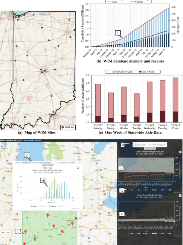
Over the last few years, Indiana has deployed data communications, computing, and storage infrastructure to process data from 33 WIM sites on INDOT road-ways. Figure 2.1a shows the WIM station locations. Data from these sites is transferred daily from the field to the INDOT TMC database. The dataset consists of a vehicle component which describes the classification and GVW, and an axle component which describes individual axle left and right-side weights. Additionally, each record has a specific location, lane number, and a 0.1-second precision detection timestamp.
Figure 2.1b shows the statewide cumulative number of vehicles and axles recorded from January 2014
through June 2017. Callout i shows a significant increase in the velocity of data coming into the system in June 2015. Currently, just over 3 billion axle records totaling around 600 GB are collected. Note that it requires slightly more storage capacity for axle records than vehicle records. Figure 2.1c shows class 9 axles separated out over a one-week period in 2017. The amount of class 9 axles increases
from 16% to 24% of the total from Saturday to the following Friday, indicating trucks getting back on the road after the holiday period.
Figure 2.1d shows an example web application visu-alizing statewide class 9 GVW and front axle data. The interface is presented on a Google Maps layer and each site is indicated by a map marker (callout i). The top of
the right-hand menu (callout ii) allows a user to select a date period for analysis, and system-wide performance is plotted on pareto-sorted graphs in the menu. Users may also get information on a particular WIM site by clicking on the WIM map marker, as seen in callouts vi and vii. Subsequent sections of this paper describe these graphs and their uses in greater detail.
2.2 Online Evaluation Methodology
2.2.1 Front Axle Confidence Band
A virtual weigh-in-motion (VWIM) concept was imple-mented using multiple sensors on an eastbound lane of I-94 just upstream of the Chesterton Indiana State Police (ISP) static weigh scales. The project team imple-mented monthly evaluations, in which over 600 class 9 vehicles were randomly sampled, weighed at ISP certi-fied weigh scales, and compared to measurements from the new I-94 VWIM system. The overall performance of the VWIM system met the expectation of¡5%error when compared to the static measurements. Over 600,000 Class 9 vehicle records were logged at this VWIM site from August to December 2016.
Front axle data is compiled and statistically analyzed from this VWIM site for the evaluation period and is summarized in Table 2.1. Front axle data from the truck-ing industry for specific models includtruck-ing the Freightliner Columbia, Kenworth T680, Volvo VN780, and Inter-national ProStar, among others, were obtained from Celadon Trucking’s Combined Weight Chart to be 10,220, 11,425, 10,900, and 11,940 pounds respectively
(Celadon Trucking, 2014). Consistent with the weights taken at the state police scales and the new VWIM station, this data is summarized in Table 2.1.
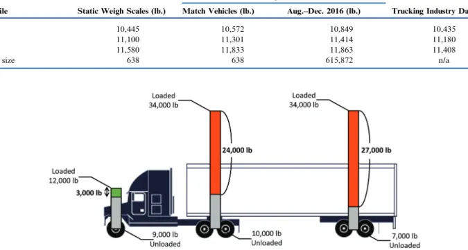
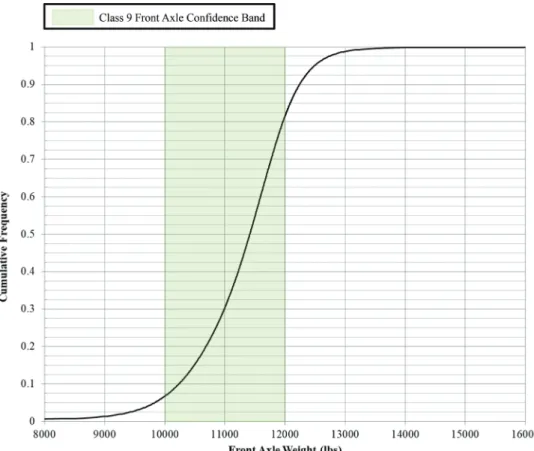
Class 9 GVW tends to have a large variance due to a variety of factors including loading conditions, weather conditions, and the commodity being transported. A class 9 vehicle can weigh as little as 30,000 pounds unloaded and up to 80,000 pounds or higher with special permits. With such a large GVW range, each individual WIM station would require custom GVW threshold values. However, as seen in Figure 2.2, the variance of class 9 front axles is much tighter and consistently between 10,000 and 12,000 pounds, regardless of the loading condition. Thus, front axle median weight is excellent for evaluating WIM performance. Front axle class 9 data from the I-94 VWIM has been plotted as a cumulative frequency diagram in Figure 2.3.
As shown in Table 2.1, a total of 615,872 class 9 vehicles are sampled to create Figure 2.3, which features a class 9 front axle confidence band ranging from 10,000 to 12,000 pounds. This confidence band captures over 75 percent of the data, and a median near 11,500 pounds.
2.2.2 Statewide Monthly Outlier Analysis
Figure 2.4 features a heat-map presenting one month of front axle weight data from ten representative WIM sites. Each row represents a single WIM lane and each column indicates a day in May. The daily median value of the front axle weight determines the color of each cell based on the front axle confidence range. Values within the range of 10,000 to 12,000 are colored white.
TABLE 2.1
Class 9 front axle weights for confidence band
I-94 Virtual Weigh In Motion Station
Percentile Static Weigh Scales (lb.) Match Vehicles (lb.) Aug.–Dec. 2016 (lb.) Trucking Industry Data (lb.)
25 10,445 10,572 10,849 10,435
50 11,100 11,301 11,414 11,180
75 11,580 11,833 11,863 11,408
Sample size 638 638 615,872 n/a
Cells are colored red for median values above 12,000 pounds and blue for values below 10,000 pounds. Greater intensity of the color indicates a greater deviance from the confidence range. This visual gives a practitioner a high-level sensor performance glance over numerous lanes for a multi-week period.
For example, callout i shows a lane that is perform-ing within range in the first half of the month, with low median values starting on May 15. Callout ii shows multiple lanes measuring slightly above range for the entirety of the month. It can be seen that these lanes belong to a single WIM site, WIM 315. Callout iii shows a lane that, for a period of two consecutive days, reads very high. This may indicate a spike in tem-perature or other weather-related conditions. Finally, callout iv shows a lane that has received no data throughout the month of May 2017. This is indicated by a line of dark grey as the query results for that lane were null.
The standard WIM lane numbering scheme employed by INDOT is shown in Figure 2.5. Lane 1 starts with the lane closest to the ITS cabinet. Lanes 2, 3, and 5 work inward toward the median. Lane numbering picks back up at the lane furthest from the ITS cabinet in the opposite travel direction and works its way to the median. Figure 2.5 shows an example of a 6-lane highway’s lane configuration. This numbering scheme can accommodate up to 10 lanes, but if there are more than 10 lanes, there will need to be an ITS cabinet on
either side of the road due to the limited number of WIM sensor inputs. In this case, both directions will be treated as separate WIM stations, and lane numbering will increase from the ditch to the median.
Another statewide WIM assessment metric is the pareto-sorted class 9 front axle median graph (Figure 2.6a). Monthly front axle median values per WIM-lane are sorted and plotted with their corresponding 75th and 25th percentile values as higher and lower error bars respectively. Callout i in part a shows the front axle confidence band in green. Approximately 70%WIM-lanes falls within this band while 20%lies above (callout ii) and 9%resides below (callout iii). Additionally plotted in this figure is the left and right sensor data. Callout iv in part a shows a confidence band for each individual left and right sensor of 5,000 to 6,000 pounds. Monthly median values for right front axle sensors are plotted in red while the left sensors are plotted in blue for each WIM-lane. A line connects the two medians for easier comparison.
Figure 2.6b shows the same WIM-lane monthly median data as a difference between the left and right sensor of each WIM lane. Callout i shows data with zero differ-ence, which may indicate a sensor failure, where the system might double the measurement of the working sensor to produce estimated truck weights. Data to the left and right of callout i that is less than 500 pounds is reasonable and expected due to the crown of the road-way and uneven loading of the trucks. Median values
Figure 2.3 Cumulative frequency diagram of class 9 front axle weights August to December 2016 on well-calibrated VWIM station.
by callout ii and callout iii are thousands of pounds different and indicate that one or both sensors are not functioning properly.
A pareto-sorted plot of the class 9 left-right residuals from the VWIM system on I-94 is shown in Figure 2.6c.
Callout iv shows the median value of 315 pounds for the data in part c. Although it is reasonable to see a difference of 300-500 pounds between left and right sensors, a residual value of 1,000 pounds or greater is atypical and indicative of a WIM sensor issue.
Figure 2.5 WIM lane configuration diagram.
2.3 Online Case Studies
2.3.1 Calibration Estimation Through Dashboard Data
INDOT has a current WIM maintenance schedule of 24 months, calibrating half of its WIM inventory every year. With such length of time between calibrations, proper calibration is crucial. Figure 2.7a shows 3.5 years of daily median front axle values from February 2014 to June 2017 for the drive lane of WIM #952100. Con-fidence bands for front axle total and front axle left/ right sensors are plotted as well as columns to indi-cate the winter months. Callout i shows one calibration that occurred on December 5, 2014, that made the
measurements less scattered. During the spring of 2015, the median front axle measurements start to increase until the next calibration (callout ii). After the calibra-tion, the median data returns to reasonable ranges and once again falls within the confidence band, indicating a successful system calibration.
This WIM site was selected for a visual inspection of the pavement and sensor conditions. Figure 2.7b shows the left quartz WIM sensor in good condition. Addi-tionally, the inductance loops, shown in part c, appear to be in good shape. Part d shows an overview of the WIM site, with the drive lane in the foreground. The asphalt was recently repaved and the pavement is in great condition.
2.3.2 Out of Tolerance Front Axle WIM Measurements and Left-Right Data
Performance metrics from the online screening tool flagged WIM#953150 (WIM 315) as being out of toler-ance. Plotting the daily median front axle data for lane 2 revealed characteristics exhibited by other lanes of this WIM station (Figure 2.8). According to INDOT’s records, the most recent calibration occurred in May 2014. Figure 2.8a callout i shows the median data at the top end of the front axle confidence band for both total and left/right weight. The left and right sensors appear to be functioning properly having consistent but not equal measurements. However, later in the winter
of 2014, data scatters and rises. Throughout most of 2015, median data tightens up, but continues a slight upward trend to end above the 12,000-pound confidence band before winter (callout ii). Seasonal variations throughout the winter months increase in severity with each passing winter and the median data continues to drift further from reasonable values.
Although front axle weight is more consistent than GVW, it should not be the only performance metric utilized. The median front axle data shown in Figure 2.8b falls within the confidence band and seems well cali-brated. However, the left-right sensor data of Lane 1 provides additional information. Starting in July of 2014, the left sensor of Lane 1 begins to measure values
above the green confidence band (callout i) while the right sensor measures values below the confidence band (callout ii). Although the sensors measure values over 1,000 pounds different, they balance each other and produce a stable total front axle graph for Lane 1. Again, winter variations are visible in the data (callout iii). However, as time passes, the left sensor begins to degrade at a faster rate than the right sensor, which has more tightly grouped data and experiences fewer out-of-range measurements.
3. PAVEMENT SMOOTHNESS IMPACT 3.1 Profiler
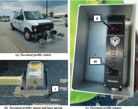
Pavement conditions also affect WIM measurement accuracy. Dynamic loading from trucks bouncing across sensors results in improper weight readings. Outlier analysis, performance metrics, and the online web application identified the top 10 most out of tolerance WIM sites throughout the state. Five WIM sites are selected and profiled by the inertial measurement profiler (Figure 3.1). Part a shows the vehicle and sensor mount while part b shows the left wheel track laser that profiles the road. There is a laser sensor on both wheel tracks that measures the distance between it and the pavement below. Each laser is about 40 wide and provides an average value along the length of the laser (callout i). This line laser covers a larger area and gives a better representation of the roadway surface than a single point laser. Callout ii is the camera lens and receiver array while callout iii is the sensor’s laser.
Each WIM lane was profiled on July 18, 2017 at a con-stant 50 miles per hour. Each WIM location was manually flagged on a laptop by clicking a button as the test vehicle passed over the WIM station. At a constant speed of 50 miles per hour (73.3 feet per second), and an average visual reaction time of 0.25 seconds, the WIM could be at least 18 feet in either direction of the marked location.
3.2 Profile of a Smooth Pavement
The pavement at the I-94 VWIM station was profiled both before and 1 year after VWIM construction in order to have a control for pavement roughness. Figure 3.2a callout i shows the location of the VWIM station. The grey line shows the pavement profile before lane grind-ing and the black line shows it after high-precision lane grinding. Callout ii shows the VWIM station after lane grinding and callouts iv and iii show a close-up of the pavement before and after lane grinding respectively.
3.3 Profile of an Unground Concrete Pavement
WIM#952300 has a rougher pavement than the I-94 VWIM station. Figure 3.3a shows each concrete panel along the roadway profile at the dotted lines. The pavement joints are set at 12-foot and 20-foot intervals. Callout i shows the location of the WIM station in parts a, b, and c of the figure. Callout ii shows a dip in the left sensor profile in part a and demonstrates the
pavement distress that is evident in part b. Part c is a satellite image of the WIM station with dotted lines that correspond to dotted lines in part a.
3.4 Transition Pavement Profile
WIM station#953150 has a much more pronounced elevation profile than the previous two. Callout i shows the location of the WIM station in Figure 3.4a and in the satellite view in part b. The jolt observed near callout ii matches up with a pavement transition from asphalt to concrete. This transition is not smooth for any of the three outside lanes. Although the distance between callout i and callout ii is more than 110 feet in the profile data, it is well within the range of possible distances based on human perception-reaction time and vehicle speed. The bumps observed in the data after the pavement transition in part a could be the van settl-ing after the jolt of the pavement transition. A video of class 9 trucks bouncing after the pavement transi-tion can be seen at the URL in part b. It is clear that
the pavement transition at callout ii causes larger vehicles to bounce which produces out-of-range WIM measurements.
3.5 Effect of Pavement Smoothness on WIM Precision
Smooth pavement is imperative for consistent, accu-rate, and precise WIM measurements. Callouts i and ii in Figure 3.5a show daily median front axle data for the I-94 VWIM station in comparison to a successfully calibrated WIM#952100. Both stations produce stable and consistent data for front axle total left and right. However, part b shows that there is a discernable dif-ference between the I-94 VWIM and the other WIM stations used as case studies in this report. The r-squared value of a best-fit line can serve as a proxy for preci-sion and approximate the scattering of the WIM data. The data in part b suggests significantly less variance in measurements from the I-94 VWIM station. This further emphasizes smooth pavement as a necessity for proper WIM measurements.
4. FIELD VALIDATION
The first field evaluation took place on Eastbound I-94 near the Chesterton State Police Weigh Scales. In May 2016, VWIM sensors were deployed and Purdue University was tasked with the third-party evaluation of the new system’s performance. Each of the 5 monthly evaluations sampled 100-150 trucks at the Indiana State Police static weigh scales, and their observations were compared to the weights measured by the WIM system. The results showed that the overall perfor-mance of the WIM system met the expectation of¡5%
error as compared to the static weigh scales at the Indiana State Police post.
Collaboration with Indiana State Police was crucial for the success of the project. In order to verify the accuracy and precision of the WIM system, it was neces-sary to weigh the trucks with certified scales. Figure 4.1 shows the collaboration between Purdue and Indiana State Police. Part a shows an Indiana State Police Officer operating the static scale. Part b shows the Commercial Vehicle Enforcement Division (CVED) static weight screens where the weights of the vehicles are displayed. Members of the Chesterton CVED team that were crucial to the success of the project are pictured in part c.
Figure 4.2a shows an example of the August monthly evaluation with 122 trucks matched and plotted. Almost all class 9 vehicle data points fit within the¡5% thresh-old. Part b of Figure 4.2 shows all 564 trucks sampled in one comparison plot. With very few exceptions, almost all the data consistently fits within the same
¡5% threshold. The individual monthly evaluations paired with the cumulative evaluation indicate that the accuracy and precision on the fresh VWIM system are within acceptable ranges.
4.1 I-70 WIM Location
The initial location for the precision and accuracy test of one of INDOT’s WIM stations was determined by considering several factors including location, prox-imity to a state police weigh station, WIM sensor age, pavement condition, and traffic counts. Figure 4.3 shows all interstate ingress lanes for the state of Indiana as well as a few major highway ingress lanes. White circles represent WIM stations while white circles with yellow stars over them represent VWIM stations that have cameras. The black car silhouette represents Indiana State Police weigh scale locations.
The top 6 WIM locations to investigate are shown in Figure 4.4, based on interstate ingress status and prox-imity of WIM to Indiana State Police weigh station. Each of these six locations were studied in greater detail to reveal that the most promising WIM station for evalua-tion is near Richmond on I-70. Figure 4.5 highlights the top reasons for recommending WIM#3700 as the primary evaluation WIM station. Although the pave-ment was not brand new, it has been recently recon-structed and the sensors were replaced during that time.
I-70 does not have the highest total traffic, however, INDOT records indicate that this portion of I-70 has the highest percentage of truck traffic. Proximity to the state police post was also a factor in the decision to recommend WIM#3700 as the evaluation station. Although it was not the closest to a weigh scale, it is the second closest, and it only has one significant highway exit in the 7-mile stretch between, as opposed to WIM
#4300, which has both US Highway 20 and US High-way 421. Therefore, the decision to use WIM #3700 near Richmond, Indiana was supported.
WIM #3700 is located on I-70 near Richmond, Indiana less than a mile west of the Indiana/Ohio state line. Figure 4.6a shows the exact location of WIM#3700 (callout i) as well as the state police post (callout ii). The sensors on the westbound lanes of I-70 WIM#3700 can be seen in part b. The state police weigh scale is pictured in part c of the figure. It should be noted that there are 3 exits between WIM#3700 and the ISP static scales. This makes proper identification of trucks challenging.
Figure 4.1 Partnership with Indiana State Police Commercial Vehicle Enforcement Division.
It is not guaranteed that a truck approaching the static scales came directly from the WIM on the interstate 7 miles back. This is purely a concern with the current practice of data collection and is solely an issue of posi-tive re-identification. For example, a truck that approaches the static scales at 12:40 pm would be assumed to cross the WIM approximately 7 minutes prior, at 12:33 pm. However, that truck may have taken an exit to refuel and eat lunch, a stop that could easily take more than 30 minutes. In this case, that truck would be found to have crossed the WIM at 12:03 pm or earlier, and its weight measurement would not be valid as additional weight in the form of fuel could have been added. Depending on the size of the truck’s tanks, a semi
tractor can hold anywhere between 100–400 gallons of fuel. At approximately 7 pounds per gallon, the differ-ence between an empty and a full gas tank could be 700–2800 pounds. Therefore, all weights of trucks not found within 10 minutes of weighing at the static scales were thrown out.
4.2 I-70 WIM Evaluation Procedure
The evaluation procedure test setup is straight-forward. A truck drives over WIM #3700 sensors at highway speeds (Figure 4.6b) and that truck will travel 7 miles to the state police weigh scale where its weight will be measured with certified scales (Figure 4.6c).
These measurements will be recorded and compared for evaluation. The WIM sensors are piezoelectric quartz crystal sensors that generate an electrical impulse as a truck drives over the sensors. They are capable of measuring the left and right components of each axle individually. However, the certified weigh scales do not have such capabilities of weight data fidelity. Figure 4.7 highlights the three pressure plates typically found at an Indiana State Police weigh scale. Callout i shows the front axle pressure plate while the drive tandem pressure plate is indicated by callout ii, and the trailer rear tandem pressure plate can be seen with callout iii. An observer must be vigilant and ensure that the truck places itself fully and correctly on the scale or incorrect weight readings will result. The weighing mechanism for the certified weigh scale is pictured in Figure 4.8. Part b shows a close-up of the calibrated pressure strain gages that measure the additional weight on each platform.
Data from WIM#3700 is recorded and permanently housed in a server at INDOT’s Traffic Management Center in Indianapolis. WIM #3700 is not a VWIM site as it only records weight data and does not have cameras to photograph vehicles as they cross the WIM. Consequently, a GoPro is deployed to record video of
every vehicle that crosses the WIM in order to posi-tively match truck weights. Figure 4.9a shows the aerial photograph of the WIM site and where the GoPro is deployed to monitor westbound traffic. Part b shows an officer in the scale house monitoring the CVED weight screen, callout i. It is nearly impossible to bring targeted vehicles into the static scales for weighing in an efficient manner. This is due to the geometry of the approach, the short exit ramp to the scale house, and line-of-sight constraints at the Richmond scale house. In order to obtain the maximum amount of matched data, trucks are brought into the static weigh scales and weighed as quickly and as safely as possible. Over a 100-minute time period, about 130 class 9 trucks were weighed at the static scales. In general, this is about 45 seconds per weighed truck.
Truck weights were recorded as they were weighed at the static scales, and GoPro video footage captured every truck that crossed the WIM station. After data collection at the static scale was finished, the video cameras were retrieved, and researchers scoured video from the WIM site for each truck that was weighed at the static scales. Figure 4.10a shows a truck being weighed at the static scales while part b shows that truck crossing the WIM station nearly 8 minutes earlier.
Figure 4.4 Indiana egress lanes with nearby State Police weigh scales and INDOT WIM systems.
Figure 4.6 WIM#3700 and State Police weigh scale location and physical condition.
Figure 4.10c shows the true weight of the vehicle obtained at the static weigh scale.
Figure 4.11 shows the research procedure for match-ing the weights of the trucks from the static scale to weights of the same truck at the WIM. Over 30 hours of back-end work was put into properly identifying and matching 300 trucks that were originally collected over 5 hours. Figure 4.11i shows images of each truck weighed at the static scale, and served as the beginn-ing of the searchbeginn-ing procedure. Callout ii shows video footage from the static scale to capture any details about the truck that the photograph cannot provide, such as the truck’s arrival time to the scale. Callout iii shows video footage at the WIM, which was viewed in order to match weights recorded at the WIM to specific trucks. Callout iv is a time synchronizing spreadsheet designed to reveal the real time of any event that occurs in the video files collected that day. It also allows
researchers to target any specific time in the videos. Figure 4.11v and vi show the WIM data that has no truck designation, which is matched by timestamp to the truck in question. Weight, speed, and temperature data from the WIM as well as weight data from the static scale are then recorded for each truck, as demon-strated in callout vii.
4.3 I-70 WIM Evaluation Results
The true gross weight of the vehicle seen in Figure 4.10 was found to be 61,480 pounds. However, the weight of that vehicle obtained by WIM #3700 was only 54,249 pounds, an 11.8%difference. In order to assess the status of the WIM, it is necessary to determine if the scale is accurate and or precise. Figure 4.12 shows the subtleties between accuracy and precision. A 12% dif-ference in vehicle weight would suggest low accuracy,
low precision, or both (Figure 4.12 parts a, b, c). How-ever, a properly functioning WIM system would have both high accuracy and high precision (part d). In order to determine whether the system has low accuracy or low precision, or both, more data must be collected. The sensors in the drive lane work independently from the sensors in the passing lanes, thus their respective measurements do not affect one another. Therefore, a lane-by-lane analysis is required. Figure 4.13a shows 57 data points collected over the course of two hours on December 20, 2017. These trucks all crossed the WIM in the drive lane only. It should be noted that most of the weights obtained by the WIM are around 10% lower than the weights obtained at the certified static scales, the true weight. There is a clear upward
trend with the data, centered around the -10%dashed line, which indicates consistency with the data. In fact, it looks like the data has a systematic bias to about 10% below the true weight. It is clear from the data that the WIM is not very accurate. The true weight of the truck is consistently incorrect. However, the data has a very small spread, even when measuring heavier trucks. This suggests that the WIM is precise (Figure 4.12b).
Although a trend is indicated by the data collected in December 2017, it is not enough data to be statistically sound. Additionally, this only samples the WIM while the temperature was nominally 39uF over a 2-hour data collection period. Therefore, additional data was col-lected on February 15, 2018 over a 5-hour period. The temperature was nominally 60uF throughout the duration
of the data collection. This study added 206 truck weights in the drive lane. Despite temperature and temporal variation, WIM#3700 continued to collect data that was consistently low, matching the graph shown in Figure 4.13a.
It is possible that the inaccuracy is a result of improper calibration. A proper WIM calibration can be statis-tically estimated through ordinary least squares (OLS) linear regression. An OLS linear regression was perfor-med on the relatively small data set as well as the larger second data set independently. The following equations were developed to statistically adjust the data using OLS regression. Equation 4.1 corresponds to the data col-lected in December while Equation 4.2 corresponds to the February data.
Y~1:0644Xz1956:6 ð4:1Þ
Y~1:155Xz107:18 ð4:2Þ
Figure 4.13b shows the transformed December data through OLS linear regression. Note that the data shifts
to be centered on the 45uequality line and the spread of the data decreases to only ¡5%. Figure 4.14 shows all transformed data for the drive lane. Referring to Figure 4.12, if this WIM were properly calibrated, it would have both high accuracy and high precision. Random error from the WIM and from the static scales is expected, and it is normal to see both positive and negative measurement discrepancies due to a variety of factors. Recall that for a new WIM installation with significant care taken during construction and calibra-tion, a¡5%error was observed. Therefore, with proper calibration it may be possible for WIM #3700 to reach similar levels of performance.
In order to better understand the true spread of the data, a cumulative frequency diagram was created for the 262 truck weights. Figure 4.15 shows a CFD plot with the adjusted percent error shown for WIM#3700 lane 3 as well as data obtained at the I-94 VWIM, ranging from -10%to nearly 8%. The plots look similar to each other, with the biggest exception being that the data from the I-94 VWIM, shown in black, only has a
spread of -6%to+6%. It should be noted that in both cases, 0%error is near 50%of the data. Therefore, the data is centered around 0 in both cases. The curves indi-cate that errors observed in the positive and negative directions are random measurement errors and there is no significant bias in either direction. Also, 90%of the data for WIM #3700 is contained within ¡5% while
over 95%of the data for I-94 is contained within¡5%. This further supports the¡5%claim from Figure 4.14. Other factors such as vehicle speed and pavement temperature have been known to affect weight mea-surements obtained by WIM technology. Figure 4.16a shows a histogram of the 206 truck speeds collected on 2/15/18. Figure 4.16b shows a bar graph of average
Figure 4.12 Visual depiction of the correlation between precision and accuracy.
percent errors binned by truck speeds. A general trend can be seen, although in the lowest and highest speeds, statistical significance is low as the sample size is less than 5 for both cases. However, it appears that lower
speeds may result in negative percent error, or the WIM measuring low. Similarly, speeds higher than 67 miles per hour may result in the WIM measuring high when compared to the static scale.
Figure 4.14 WIM#3700 GVW and static scale true GVW adjusted values.
5. DISCUSSION AND CONCLUSIONS 5.1 Discussion
Seasonal variations were observed in the daily median front axle data of many WIM stations over the 3.5-year dataset. INDOT calibrates its WIM stations on a bi-annual basis, in the fall of every other year. During the winter months, the median weight data tends to become less accurate and less precise due to temperature variations among other factors. Pavement transitions should be avoided within close proximity of the WIM stations because they cause vehicles to bounce over the scales, resulting in incorrect measurements. Pavement smooth-ness is crucial to obtaining accurate and precise WIM measurements. At highway speeds, truck suspensions should dampen bounces due to shocks within a few seconds. At 70 miles per hour (103 feet per second), two seconds would require at least 200 feet of smooth pavement before the WIM station.
A field validation project was completed for two sepa-rate WIM stations, one brand new construction on I-94 near Chesterton, and one reconstructed WIM station near Richmond, Indiana. The new construction near I-94 utilized specialized vendor-specific VWIM equip-ment and specified an extremely tight construction tolerance that was practically unattainable and was not scalable for a statewide system. The study collected 564 static weights and found that over 98% of the VWIM weights were within¡5%of the static weights, as expected. The recent reconstruction of the INDOT WIM #3700 near Richmond, Indiana was not dis-covered to be within vertical tolerance according to American Society for Testing Materials (ASTM) when profiled by INDOT. However, a field validation was also completed for this WIM as a gauge for INDOT’s current practices. The study collected 262 static weights and found that all the WIM weights were systemati-cally low by about 10%to 15%when compared to static weights from the ISP static scales. This systematic bias is most likely a result of poor calibration. An ordinary least squares linear regression was applied to all 262 WIM weights to statistically approximate a properly calibrated station. After statistically adjusting the data, 87%of the WIM weights were found to be within¡5%
of the static weights. These results are encouraging, as they indicate that such precision and accuracy may nearly be achieved with slightly more attention to quality assurance and quality control of reconstruction at the site. With improvements in communication, data proces-sing, and data storage, it is more possible to observe and predict trends in commercial vehicle weights state-wide. As commercial vehicle information becomes more available, agencies will have a better ability to observe and act upon habitual offenders of weight limits and other permitting violations. Data is recorded and avail-able in near real-time. Real-time dashboards can be created that approximate statewide WIM system health as well as highway infrastructure system health. Each WIM records the weight of commercial vehicles as they travel that section of highway. It is possible to create a
real-time dashboard that shows the approximated remaining service life of each roadway section. Further-more, with the addition of specialized equipment, such as license plate readers and Department of Transporta-tion (DOT) number readers, the resoluTransporta-tion of the data can be brought to specific trucking companies, and even individual drivers. Therefore, there is great potential to target individuals that routinely violate weight limits on individual axles or on gross vehicle weight. Utilizing such technologies may give agencies a more effective way to discourage future violations and preserve the integrity of the highway infrastructure for the future.
5.2 Conclusions
INDOT processed data for 33 WIM/VWIM sites throughout the state which produced approximately 550 million total vehicle records per year in 2016. Several performance metrics have been proposed on limited data sets in past studies (Nichols & Bullock, 2004; Nichols et al., 2009; Nichols & Cetin, 2007). This study implemented an online WIM health-monitoring tool (Figure 2.3) and examined five areas.
N
Validation and use of the class 9 front axle weightN
Validation and use of the left-right front axle residualN
Impact of pavement smoothing on WIM performanceN
Field validation on recently constructed vendor-specificVWIM
N
Field validation on recently renovated INDOT WIM siteClass 9 GVW tended to have a large variance depend-ing on a variety of factors includdepend-ing the loaddepend-ing, weather, and commodity transported. However, the front axle of class 9 vehicles tends to have a much tighter variance and consistently ranges between 10,000 and 12,000 pounds regardless of overall GVW.
Diagnostic tools analyzing median front axle weight of class 9 vehicles were used to assess overall system health. These performance measures were used to evaluate specific WIM stations and individual sensors. Seasonal variations were observed for one station with increased variation during the winter months. In another station, even though overall front axle weights were in range, left-right sensor measurements were observed to be dramatically different which emphasized the need to examine sensors on each wheel track separately.
Pavement profiling was performed to further determine the root cause of out-of-range data. The VWIM station on I-94 was profiled before and after lane and was found to have a¡5%accuracy after lane grinding. In contrast, the profile of a WIM station that is close to a transition from asphalt to concrete pavement shows high pavement profile variations. The I-94 VWIM had a best fit r-squared value of 0.03 after lane grinding WIM stations with significantly rougher pavement had wider spread data with best fit r-squared values between 0.3 and 0.5. Wider spread data indicates low precision, reinforcing the need for smooth pavement just before and at WIM sites.
Field validation tests were performed on two sepa-rate WIM stations, one vendor-specific VWIM site using
tight construction tolerances and requiring significant effort in calibration, and one recently rebuilt INDOT WIM using current construction tolerances and cali-bration techniques. It was determined that the vendor-specific VWIM site had slightly greater precision cap-abilities than the INDOT WIM. However, the accuracy of the INDOT WIM was not within acceptable ranges due to poor calibration. Statistical adjustment of the INDOT WIM data revealed the potential for nearly 90%of the data to fall within¡5%when compared to static weights with 95%of the data falling within¡7%. Such accuracy and precision was achieved on a WIM station that did not meet ASTM standards for pave-ment smoothness. This indicates that better accuracy and precision can be achieved on sites with pavement that meet ASTM smoothness standards.
6. ACKNOWLEDGMENTS
This work was supported by the Joint Transpor-tation ResearchProgramandtheIndianaDepartment ofTransportation.Thecontentsofthispaperreflectthe viewsofthe authors,whoare responsibleforthefacts andthe accuracyofthe datapresented herein, anddo notnecessarilyreflecttheofficialviewsorpoliciesofthe sponsoring organizations. These contents do not con-stitute astandard,specification, or regulation.VWIM datawasprovided byKapschTrafficCom.
REFERENCES
AASHTO MP 14-05. (2012). Standard specification for smoothness of pavement in weigh-in-motion (WIM) systems. Washington, DC: American Association of State Highway and Transportation Officials.
Al-Suleiman, T., Sinha, K. C., & Kuczek, T. (1989). Effects of routine maintenance expenditure level on pavement service life.Transportation Research Record,1216, 9–17.
ASTM E1318-09. (2017). Standard specification for highway weigh-in-motion (WIM) systems with user requirements and test methods. West Conshohocken, PA: ASTM International. Celadon Trucking. (2014, October 1).Combined weight chart. Accessed July 30, 2017, at https://www.celadontrucking.com/ cms400min/celadon2013/pdfs/combined-weight-chart.pdf
Cunagin, W. D. (1986). Use of weigh-in-motion systems for data collection and enforcement (NCHRP Synthesis 386). Washington, DC: Transportation Research Board. Dahlin, C. (1992). Proposed method for calibrating
weigh-in-motion systems and for monitoring that calibration over time.Transportation Research Record,1364, 161–168. Dossey, T., Easley, S., & McCullough, B. F. (1996).
Methodology for estimating remaining life of continuously reinforced concrete pavements. Transportation Research Record,1525, 83–90. https://doi.org/10.3141/1684-06 FHWA. (2010).WIM data analyst’s manual(Publication No.
FHWA-IF-10-018). Washington, DC: U.S. Department of Transportation, Federal Highway Administration. Lee, C. E., Izadmehr, B., & Machemehl, R. B. (1985).
Demonstration of weigh-in-motion systems for data collection and enforcement(Report No. 557-1F). Austin, TX: University of Texas at Austin.
Lee, C. E., & Machemehl, R. B. (1985). Weighing trucks on axle-load and weigh-in-motion scales. Transportation Research Record,1048, 74–82.
Moore, R. C., Stoneman, B. G., & Prudhoe, J. (1989). Dynamic axle and vehicle weight measurements: Weigh-in-motion equipment trials. Traffic Engineering and Control,
30(1), 10–18.
Nichols, A. P., & Bullock, D. (2004). Quality control pro-cedures for weigh-in-motion data (Joint Transportation Research Program Publication No. FHWA/IN/JTRP-2004/12). West Lafayette, IN: Purdue University. https:// doi.org/10.5703/1288284313299
Nichols, A. P., Bullock, D., & Schneider, W. (2009). Detecting differential drift in weigh-in-motion wheel track sensors.
Transportation Research Record,2121, 135–144. https://doi. org/10.3141/2121-15
Nichols, A. P., & Cetin, M. (2007). Numerical characteriza-tion of gross vehicle weight distribucharacteriza-tions from weigh-in-motion data. Transportation Research Record,1993, 148– 154. https://doi.org/10.3141/1993-20
Papagiannakis, A. T. (2010). High speed weigh-in-motion calibration practices. Journal of Testing and Evaluation,
38(5), 615–621.
ProVAL. (n.d.). Implementation of ProVAL OWL: A tech brief. Retrieved May 4, 2018, from http://www.roadprofile. com/download/Implementation-of-OWL.pdf
Stiffler, W. W., & Bensly, R. C. (1956). Weighing trucks in motion and the use of electronic scales for research.Traffic Engineering,26(5), 195–199, 206.