Modeling Gentrification: an Agent-Based, Amenities-Driven
Approach
Avishai Halev
Supervisor: Nancy Rodriguez
1
Abstract
The evolution of urban areas plays a major role in crafting public policy and spurring investment. Gentrification, involving the “transformation of a working-class or vacant area of the central city into middle-class residential or commercial use”1 , is inherently inter-twined with neighborhood ascent and descent. We propose an agent-based model to study the existence and dynamics of gentrification, centered on a two-dimensional lattice with wealth and an inherent amenities interacting via particular feedback processes. Various parameter regimes beget distinct sets of dynamics, including that of wealth hotspots – as consistent with empirical observation. We then derive a continuum model of partial differ-ential equations (PDE) from the agent-based model and analyze the instability regime of the continuum system; the resultant regime agrees with observations of simulation of the discrete model.
2
Introduction
Gentrification is well-documented as a major factor in modern urban development. This residential phenomenon is associated with major increases in housing prices and upgrades of local amenities, leading to an emigration of low-income residents and an influx of wealthier community members. This wealthier contingent is generally whiter, more educated, and younger compared to the low-income residents they replace2.
While the existence of gentrification is a hot topic in political circles, its underlying causes and effects are wildly disputed. An inability to study the problem experimentally and the potential for a wide variety of motivating factors complicate any deep under-standing of the issue. Hamnett (1991) suggested three main drivers for gentrification – the existence of middle-class potential gentrifiers, an availability of urban housing, and a tendency among these potential gentrifiers to prefer to live in an urban setting3. Other proposed drivers of gentrification include falling crime rates in inner city neighborhoods4,5,
demanding work schedules and lack of free time among the young middle class6, proximity to social amenities, such as coffee shops, beer gardens, bike shares, gyms and restaurants7, and increased racial tolerance among Millennials8.
Further obfuscating an empirical understanding of gentrification is the potential pres-ence of inherently chaotic dynamics9–11. Despite this, the majority of theoretical analysis of gentrification has focused on binary divisions – blacks and whites, flows of capital and flows of people, macro-forces of capital accumulation – concentrating on subsets of the potential dynamics involved in gentrification2,12.
Typically, modeling gentrification involves agent-based models that allow virtual simu-lation in lieu of experiment; the seminal ”Schelling model” of residential segregation utilized an agent-based model inhabiting an 8x8 lattice with two classes of agents to represent an arbitrary binary social division13,14. The Schelling model found that segregation was ram-pant even in situations where agents were willing to inhabit neighborhoods that consisted of up to two thirds of the other group13,14.
Extensions of the Schelling model to examine a variety of issues related to residential segregation and gentrification focused on similar agent-based approaches15–18. However, the discrete nature of the agent-based model prevents the implementation of various ana-lytical techniques to better understand such a system.
Hasan and Rodriguez (under review) proposed a model of gentrification using parabolic PDEs19. Their work, centered on the assumption that wealth diffuses but is also advected by an amenity-driven velocity field, showed that relevant parameter regimes exist that lead to wealth hotspots. This model, however, suffers from the lack of a derivation from underlying first principles.
PDEs are a valuable tool to model the spatiotemporal dynamics of ecological and sociological systems20,21, and the derivation of PDE systems from agent-based models has
proven to be effective in a range of mathematical applications, particularly in mathematical biology22–24. Short et. all (2008) considered agent-based and continuum (PDE) models of criminal behavior and showed that the two systems were in agreement in the limit of large system sizes25.
3
Discrete Model
This section is devoted to the introduction of a discrete model for the dynamics of wealth in a given community — measured in dollars as incomes or net worth — and an intrinsic, dimensionless amenities, meant to encompass the variety of spatial factors involved in gentrification – from proximity to work to the density of coffee shops and restaurants6,7.
We consider this community to be a two-dimensional lattice; for simplicity’s sake, we consider a rectangular grid lattice with constant lattice spacing ` and time step δt, with each lattice site shaving a given wealthWs(t) and amenities As(t).
If unmaintained, we expect amenities to decay in time with decay rate ω. However, attractive features will increase proportionally to the wealth at a given site, due to in-stitutional factors such as increases in property taxes and effectiveness of home owners associations. Newer, wealthier residents may also demand improved or different goods and services; prompting an influx of new retailers – who expand, provided residents have the capital to sustain them26,27. We thus introduce φ as a parameter measuring the rate of increase in amenities, per dollar, per unit time; as a result, we model this growth and decay by
As(t+δt) =As(t)(1−ωδt) +φWs(t)δt. (1) Certain sources of investment – in particular, those originating in the private sector – are highly sensitive to the likelihood of return on investment and thus on the level of current wealth. Other sources, however, are more stable; public investment in infrastructure – such as schools, parks, highways, and rail transit – play a role in the gentrification of neighborhoods2,28. We model this stable, external investment by allowing our amenities to grow at a constant rate Γ>0.
As a phenomenon, gentrification does not occur at isolated sites; rather, a wealth of literature shows that neighborhoods are often segregated by socio-economic class29–32. Neighborhood amenities not only affect the site they are located at but adjacent sites as well; we model this association by modifying our update rule to allow As to spread to its neighbors. Specifically, we introduce a parameter η that varies between zero and unity that measures the relative strength of neighborhood effects and alter our update rule:
As(t+δt) =
"
(1−η)As(t) +
η z
X
s0∼s
As0(t)
#
(1−ωδt) +φWs(t)δt+ Γδt (2)
wherezis the coordination number – denoting the number of sites adjacent tos– and the sum is taken over all sites s0 that neighbor s.
We devise a similar update rule to model wealth, beginning with a stipulation similar in form to (1). We expect wealth to decay in time at the same rate as amenities, and reinvestment to occur proportionally to the wealth at that site. In lieu of a constant of proportionality, we consider a proportionality functionr(Ws;As):
Ws(t+δt) =Ws(t)(1−ωδt) +r(Ws;As)Ws(t)δt. (3)
Different forms of r(Ws;As) may be adopted to better model particular municipalities or underlying factors. As examples one may consider
r(Ws) = ˜r
1− Ws M
(4)
or
r(Ws;As) = ˜r
1−Ws M
Ws
M −As
(5)
where ˜r and M parameters.
We implement neighborhood effects in a similar manner as we have done for the ameni-ties. Research has shown that property values, in particular, rise in accordance to their proximity to quality schools and parks33,34 and highways35. We argue that neighborhood effects are skewed towards sites with amenitiesAs that are high relative to all neighbors of a given sites0.
Our update rule for wealth is thus:
Ws(t+δt) =
"
(1−η)Ws(t) +ηAs(t)X s0∼s
Ws0(t)
P
s00∼s0As00(t)
#
(1−ωδt) +r(Ws, As)Ws(t)δt.
(6)
3.1 Logistic Growth
From this point, we consider a logistic rate of reinvestment of the form:
r(Ws) = ˜r
1− Ws M
(7)
with ˜r a constant growth rate and M a carrying capacity. This choice of reinvestment rate is motivated by our expectation of two distinct regimes:
1. Direct, external sources of investment — such as government funding and philan-thropy — are targeted towards areas of lower wealth. These sources are highly mo-tivated by return on investment; if low-wealth areas are seen to improve with direct investment, investment will increase up to a certain point.
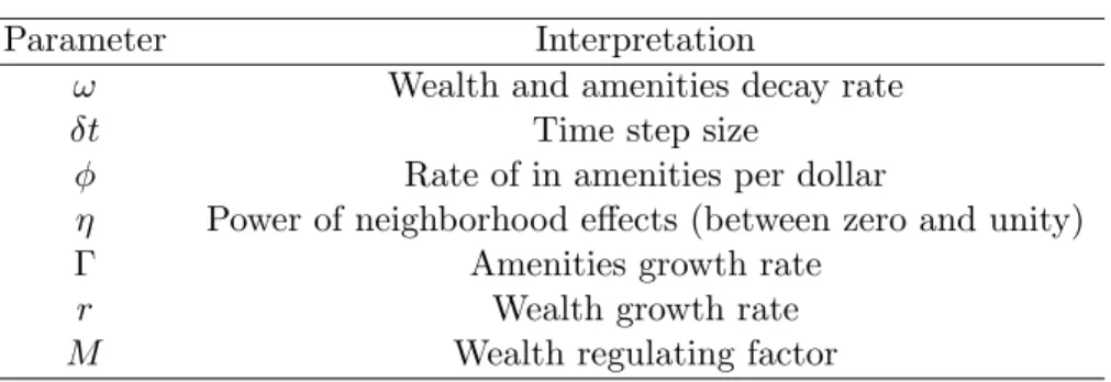
Table 1: Discrete Parameters
Parameter Interpretation
ω Wealth and amenities decay rate
δt Time step size
φ Rate of in amenities per dollar
η Power of neighborhood effects (between zero and unity)
Γ Amenities growth rate
r Wealth growth rate
M Wealth regulating factor
As such, we have the following update rule, where we have dropped the tilde:
Ws(t+δt) =
"
(1−η)Ws(t) +ηAs(t)X s0∼s
Ws0
P
s00∼s0As00
#
(1−ωδt) (8)
+r
1−Ws(t) M
Ws(t)δt.
Equations (2) and (8) form the main components of our discrete system with logistic rate of reinvestment. We employ no flux boundary conditions, so that no wealth or ameni-ties is lost through the boundaries; all sources and sinks are contained within the governing equations. The relevant parameters are summarized in Table 1.
3.1.1 Discrete Solutions
With this system, we have two spatially homogeneous solutions:
Ws As = 0 Γ ω (9) and Ws As =
M1− ωr
M φ ω
1−ω r
+Γω
Note that if ωr = 1 our two solutions collide, whereas they are otherwise distinct. As such, we can predict a transcritical bifurcation at this point, pending the stability of these spatially homogeneous solutions. In order to determine whether these spatially homogeneous solutions are stable, and to analyze the potential bifurcation about the point ω
r = 1 we run simulations on this system for various parameter regimes as detailed below.
3.2 Discrete Simulations
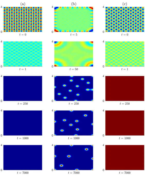
Simulations of our discrete system (2) and (8) are run in MATLAB on an 100x100 rectan-gular lattice with spacing`= 1 and time stepδt= 0.01 with periodic boundary conditions. By varying our parameters, we observe three distinct sets of dynamics:
1. Homogeneous destitution. In this case, both the amenities and wealth decay
through-out, and the entire domain quickly approaches our first spatially homogeneous solu-tion given in (9). In particular, we observe homogeneous destitusolu-tion persist in the regime ωr ≥1, considering only positive values of these parameters.
2. Homogeneous wealth. Here, amenities and wealth quickly converge to the second
solution given in (9). This regime materializes for 0< ωr <1; while the homogeneous wealth solution exists for ωr > 1, it takes on negative values in this regime and appears to be unstable to small perturbations; simulations with ωr > 1 and with the homogeneous wealth solution as initial condition eventually diverge as numerical errors accumulate.
3. Wealth hotspots. In this regime, spatial homogeneity is not achieved in reasonable
time scales. Small pockets of wealth and amenities are surrounded by large areas of destitution. These hotspots form early and quickly become circular. However, achieving temporal stability can take significant time, with hotspots deforming and merging in the process before returning to their circular state. The parameter regime leading to hotspots appears to be 1−ε < ω
r <1, whereε >0 is small and may depend on other parameters or initial conditions.
Figure 1: Output of the discrete simulation for η = 0.01, Γ = 0 in the three distinct parameter regimes. Left, homogeneous destitution, ωr = 0.9. Center, hotspots, ωr = 1.1. Right, homogeneous wealth,ωr = 1.3.
4
Continuum Limit
In order to examine the dynamics of the system in greater detail, we derive a continuum system from the agent-based model. We begin by rewriting equation (2) as
As(t+δt) =
As(t) +
η`2
z ∆As(t)
(1−ωδt) +φWs(t)δt+ Γδt. (10)
where ∆As(t) is the discrete spatial Laplacian:
∆As(t) =
X
s0∼s
As0(t)−zAs(t)
!
/`2. (11)
We now subtract As(t) from both sides, convertWs(t) into a wealth density W(t) by dividing by`2, and divide through by δt. Taking limits asδt, `2 → 0, and requiring that
D=`2/δt and ϕ=`2φremain constant, we arrive at our continuous amenities equation:
∂A ∂t =
ηD
z ∆A−ωA+ϕW + Γ. (12)
By performing a series of similar – if slightly more involved – operations, we arrive at our continuous equation for the wealth density (see appendix for details):
∂W ∂t =
ηD z
h
∆W −2∇ ·(W∇logA)
i
+r
1−W M
W −ωW. (13)
Equations (12) and (13) combine to form a system that serves as a continuous corollary to the agent-based model; they are of the general form of a reaction-diffusion system, sys-tems that often beget pattern formation36. The amenities diffuse spatially while decaying in time; simultaneously, higher levels of wealth and external sources lead to investment in the amenities of a community. Wealth also diffuses spatially and decays in time; wealth reinvestment occurs if the level of wealth is below a certain carrying capacity, that, if exceeded, leads to an additional sink of wealth.
4.1 Dimensionless Equations
To better understand the intrinsic properties of the system, we non-dimensionalize using the characteristic time scaleτ ≡1/ωand length scale`c≡
p
D/ω, arriving at the following scaled variables:
˜
A= ω
ϕMA, W˜ =
1
MW, x˜= √
z `c
x, t˜=ωt. (14)
Our dimensionless equations are thus
∂W
∂t =η[∆W −2∇ ·(W∇logA)] +ρ(1−W)W −W, (15) ∂A
whereρ≡r/ω andγ ≡Γ/(ϕM).
This non-dimensionalization has reduced our parameter space from the original eight dimensional parameters to three non-dimensional, and our three dimensionless parameters have clear interpretations in terms of our dimensional variables. Our originally dimension-less parameterη measures the strength of neighborhood or diffusive effects in the discrete and continuous simulations, respectively. The parameterρ≡ r
ω measures the relative rates of investment and decay; ρ > 1 implies excess wealth should be available in the domain while ρ < 1 suggests decay may overwhelm investment. Finally, the parameter γ is a external rate of investment in amenities that is spatially and temporally homogeneous.
In this dimensionless system, our spatially homogeneous solutions are (W , A) = (0, γ) (homogeneous destitution) and (W , A) = (1−1ρ,1−1ρ+γ) (homogeneous wealth). In terms of our dimensional parameters, these solutions are
W A = 0 Γ φM W A =
1−ωr
1−ω r +
Γ
φM
(16)
Note the resemblance between the solutions of the continuum equations above and the equilibrium solutions of the discrete system in (9). Again, depending on the stability of spatially homogeneous solutions aboutρ≡ r
ω = 1, we can predict a transcritical bifurcation at this point. More importantly, the resemblance between these equilibrium solutions suggests that results of analysis of the continuum model will carry over to the agent-based model, particularly as it pertains to analysis of the stability of these solutions.
4.2 Numerical Simulation
Numerical simulation is performed via the finite element method using a triangular mesh. Equations are solved on a grid with Neumann (no flux) boundary conditions.
Simulations of our continuum system exhibit striking similarity to their counterpart in the discrete system. In particular, systems withρ < 1 exhibit decay to the homogeneous destitution solution, while takingρ >1 will either lead to hotspots or homogeneous wealth for ρ sufficiently close to unity and larger ρ respectively. These three regimes correlate with the dynamics of the discrete system, both in terms of the observed dynamics and the parameters that give rise to them.
Spatial dynamics for various sets of parameters corresponding to those used in the discrete simulation can be seen in figure (2). The visible similarity indicates that our continuum model is an accurate approximation of our discrete equations for small time steps and spacing. Encouraged by the ability of our continuum system to predict results of our discrete system, we turn to analysis of our continuum equations to attempt to distinguish systems that exhibit hotspots from those that do.
4.3 Linear Order Analysis
To better understand the behavior of our system surrounding these equilibrium solutions, we consider values of our variables slightly perturbed from their steady states. We start with our homogeneous wealth solution (W , A) = (1−1
ρ,1−
1
ρ+γ) by analyzing perturbations of the form
A(x, t) = 1−1
ρ +γ+δAe
σteik·x,
W(x, t) = 1−1
ρ +δWe
σteik·x,
By inserting these perturbations into our dynamical equations (15) and discarding nonlin-ear terms, we arrive at the following eigenvalue equation:
−η|k|2−ρ+ 1 2η|k| 2(1−
ρ) 1−ρ(γ+1)
1 −η|k|2−1
δW δA
=σ δW δA (17)
For our system, linear order instabilities exist if the determinant of this matrix is negative:
η2|k|4+η|k|2
ρ+ 2−2ρ
γρ+ρ−1
+ρ−1<0 (18)
This is true if our amenities reinvestment γ lies within the range
1
ρ −1< γ <
−(ρ−5)(ρ−2)ρ−4p(ρ−1)3+ 4
(ρ−2)2ρ (19)
providedρ >1 or, for 0< ρ <1
γ 6= 1
ρ −1 (20)
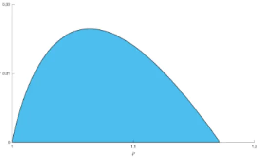
If we additionally require that our amenities reinvestment γ be nonnegative, we find that the inequality (19) is only satisfied for the bounded band given by 1< ρ <4−2√2. Thus, instabilities in our homogeneous wealth solution may exist for all reinvestments in the range 0 < ρ < 4−2√2; in particular, this instability holds for almost all γ ≥ 0 if 0 < ρ < 1. This result reinforces the value of our model as the homogeneous wealth solution (W, A) = (1−1ρ,1−1ρ+γ), which implies uniform, negative wealth for 0< ρ <1, is never attracting.
To gain a complete picture of the stability of solutions, we perform a similar linear stability analysis on the solution (W , A) = (0, γ). We arrive at the following matrix equation:
Figure 3: Instability region of the homogeneous wealth solution. Values of the reinvestment parametersγ and ρ lying in the shading region beget linearly unstable modes.
−η|k|2+ρ−1 0
1 −η|k|2−1
δW
δA
=σ
δW
δA
(21)
From this system, we find that our (0, γ) solution exhibits instabilities only if
ρ >1 (22)
If this holds, unstable modes are given by all wavenumbers such that
|k|2 < ρ−1
η (23)
Taken together, equations (19) and (22) allow us to paint a broad picture of hotspots dependent on our reinvestment parametersρ and γ. Forρ <1, there is insufficient invest-ment in the neighborhood for anyone to maintain a modicum of wealth, and both wealth and amenities decay in time until the neighborhood is destitute in wealth if not amenities. Two situations arise in the regime 1 < ρ < 4 −2√2, dependent on our amenities reinvestment γ. For sufficiently small γ – as defined in (19) – some families are able to retain their wealth; however, reinvestment is insufficient to allow wealth to prevail domain-wide and wealth is concentrated in hotspots. On the other hand, larger values ofγ allow homogeneous wealth throughout for allρ >1.
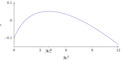
0 3 |k|2
∗ 6 9 12
−0.1 0 0.1
|k|2
σ
Figure 4: Maximum eigenvalue is plotted for a set of parameters η= 0.1, ρ= 1.1,γ = 0. The maximal wavenumber|k|∗ sets the final size of hot spots.
0 0.5 11 4 - 2√2 2
−0.4
−0.2 0 0.2 0.4 0.6 0.8 1
ρ
A
Figure 5: Transcritical bifurcation in amenities, shown here for γ = 0. Red and blue lines represent homogenous destitution and homogeneous wealth, respectively; solid and dotted lines denote regions of stable and unstable solutions, respectively. Asγ increases, the instabilities in the homogeneous wealth solution disappear, with the hotspot region 1< ρ <4−2√2 collapsing inward.
5
Conclusion
Starting from basic sociological assumptions surrounding the spread of gentrification, we derive an agent based model of this phenomenon. Namely, we consider a system wherein wealth in a community begets an increase in community investment, and vice versa. To this end we define the amenities of a community to be a measure of the results of this investment; these amenities may include various factors such as coffee shops, parks, tapas restaurants, and local festivals and events.
We argue that these amenities both diffuse spatially over time and decay temporally if not maintained; reinvestments to maintain these amenities are proportional to the amount of wealth at a given time. In particular, we focused on a logistic rate of reinvestment; future analyses may consider the effects of different such rates. Similarly, wealth travels up amenities gradients and concentrates in areas of high amenities. From this discrete empirical model, justified on sociological observations, we derive a continuous model; the resultant system of partial differential equations is of the general form of a reaction-diffusion system. For corresponding parameters we observe similar dynamics in the discrete and continuous model, and the homogeneous solutions of both discrete and continuum models are clearly alike, in their respective parameter spaces.
In both discrete and continuous models, the interplay between wealth and amenities creates a feedback loop that, for certain parameter regimes, leads to hotspot formation evocative of those observed in true gentrified neighborhoods. For the logistic rate of rein-vestment under consideration, this regime is 1< ωr <4−2√2 under the assumption that there is no wealth-independent reinvestment in amenities. By recognizing the term ωr as the ratio of investment and decay rates, we are able to qualitatively interpret the relevant regimes of this ratio. For 0 < ωr < 1, decay dominates reinvestment throughout our do-main and wealth vanishes throughout for large time scales. For ωr >4−2√2, reinvestment sufficiently overcomes decay so that wealth approaches the solution 1− ωr in a spatially homogenous fashion. The regime 1< ωr <4−2√2 begets hotspot formation with the size of hotspots determined bysomething .
We have succeeded in designing a model that exhibits qualitative similarities with empirical observations; areas of future work may involve analysis of the efficacy of our model in mirroring actual gentrification. The difficulty in devising effective measures and compiling empirical data sets is an immediate obstacle to accomplishing this; this goal is additionally complicated by the wide variety of underlying factors of gentrification. We have unified these in the ”amenities” metric but it is unclear what exactly these factors are and how significant of a role each plays in combining to form amenities.
Splitting amenities into public policy driven amenities and private investment driven amenities is another avenue worth exploring; the contrast in effective time scales between the two make this a natural division. The former would act on longer time scales and concentrate mainly on areas of low wealth while the latter would play out in shorter periods of time and invest mainly in areas where high returns on investment would be expected.
Another natural area of further inquiry would be to analyze different forms of the rate of reinvestmentr(Ws, As). Modifications ofr(Ws, As) would lead to different equilibrium solutions and sets of dynamics and could better factor in the myriad of causes of gentrifi-cation in actual cities, as well as the unique domains of particular urban areas.
In summary, our model of gentrification effectively models the creation of wealth hotspots seen in actual cities. Our ideas can serve as a basis for further inquiry into the factors leading to gentrification, which continue to be elusive. Better understanding of these factors can shape public policy to better serve those effected by this sociological phenomenon.
References
[1] Loretta Lees, Tom Slater, and Elvin Wyly. Gentrification. Routledge, 2013.
[2] Miriam Zuk, Ariel H Bierbaum, Karen Chapple, Karolina Gorska, Anastasia Loukaitou-Sideris, Paul Ong, and Trevor Thomas. Gentrification, displacement and the role of public investment: a literature review. In Federal Reserve Bank of San
Francisco, 2015.
[3] Chris Hamnett. The blind men and the elephant: the explanation of gentrification.
Transactions of the Institute of British Geographers, pages 173–189, 1991.
[4] Samuel Dastrup and Ingrid Gould Ellen. Linking residents to opportunity: Gentrifi-cation and public housing. Cityscape, 18(3):87, 2016.
[5] Ingrid Gould Ellen, Keren Mertens Horn, and Davin Reed. Has falling crime invited gentrification? Technical report, Center for Economic Studies, U.S. Census Bureau, 2017.
[6] Lena Edlund, Cecilia Machado, and Maria Micaela Sviatschi. Bright minds, big rent: gentrification and the rising returns to skill. Technical report, National Bureau of Economic Research, 2015.
[7] Victor Couture and Jessie Handbury. Urban revival in America, 2000 to 2010. Tech-nical report, National Bureau of Economic Research, 2017.
[8] Derek Hyra. Commentary: Causes and consequences of gentrification and the future of equitable development policy. Cityscape, 18(3):169, 2016.
[9] Damaris Rose. Rethinking gentrification: Beyond the uneven development of Marxist urban theory. Environment and planning D: Society and Space, 2(1):47–74, 1984.
[10] Robert A Beauregard. The chaos and complexity of gentrification. In Neil Smith and Peter Williams, editors, Gentrification of the city, chapter 3, pages 35–55. Allen & Unwin, 1986.
[11] Loretta Lees. In the pursuit of difference: representations of gentrification.
Environ-ment and planning A, 28(3):453–470, 1996.
[12] Stephen Benard and Robb Willer. A wealth and status-based model of residential segregation. Mathematical Sociology, 31(2):149–174, 2007.
[13] Thomas C Schelling. Dynamic models of segregation. Journal of mathematical
soci-ology, 1(2):143–186, 1971.
[14] Thomas C Schelling. Micromotives and macrobehavior. WW Norton & Company, 2006.
[15] Alexander J Laurie and Narendra K Jaggi. Role of ’vision’ in neighbourhood racial segregation: a variant of the schelling segregation model. Urban Studies, 40(13):2687– 2704, 2003.
[16] Romans Pancs and Nicolaas J Vriend. Schelling’s spatial proximity model of segrega-tion revisited. Journal of Public Economics, 91(1-2):1–24, 2007.
[17] Junfu Zhang. Residential segregation in an all-integrationist world. Journal of
Eco-nomic Behavior & Organization, 54(4):533–550, 2004.
[18] Elizabeth E Bruch and Robert D Mare. Neighborhood choice and neighborhood change. American Journal of sociology, 112(3):667–709, 2006.
[19] Ali Hasan and Nancy Rodr´ıguez. Transport and concentration of wealth: modeling an amenities-based theory. Under review.
[20] MA Lewis, KAJ White, and JD Murray. Analysis of a model for wolf territories.
Journal of Mathematical Biology, 35(7):749–774, 1997.
[21] H Berestycki and J-P Nadal. Self-organised critical hot spots of criminal activity.
European Journal of Applied Mathematics, 21(4-5):371–399, 2010.
[22] Nicola Bellomo, Abdelghani Bellouquid, Juan Nieto, and Juan Soler. Multicellular biological growing systems: Hyperbolic limits towards macroscopic description.
[23] Yasmin Dolak and Christian Schmeiser. Kinetic models for chemotaxis: Hydrody-namic limits and spatio-temporal mechanisms. Journal of mathematical biology, 51 (6):595–615, 2005.
[24] Radek Erban and Hans G Othmer. From individual to collective behavior in bacterial chemotaxis. SIAM Journal on Applied Mathematics, 65(2):361–391, 2004.
[25] Martin B Short, Maria R D’orsogna, Virginia B Pasour, George E Tita, P Jeffrey Brantingham, Andrea L Bertozzi, and Lincoln B Chayes. A statistical model of crim-inal behavior. Mathematical Models and Methods in Applied Sciences, 18(supp01): 1249–1267, 2008.
[26] Karen Chapple and Rick Jacobus. Retail trade as a route to neighborhood revitaliza-tion. Urban and regional policy and its effects, 2:19–68, 2009.
[27] Daniel Monroe Sullivan and Samuel C Shaw. Retail gentrification and race: The case of Alberta Street in Portland, Oregon. Urban Affairs Review, 47(3):413–432, 2011.
[28] Gary Bridge, Tim Butler, and Loretta Lees. Mixed communities: Gentrification by
stealth? Policy Press, 2012.
[29] Douglas S Massey and Nancy A Denton. American apartheid: Segregation and the
making of the underclass. Harvard University Press, 1993.
[30] Camille Zubrinsky Charles. The dynamics of racial residential segregation. Annual
review of sociology, 29(1):167–207, 2003.
[31] Claude S Fischer, Gretchen Stockmayer, Jon Stiles, and Michael Hout. Distinguishing the geographic levels and social dimensions of us metropolitan segregation, 1960–2000.
Demography, 41(1):37–59, 2004.
[32] Richard Fry and Paul Taylor. The rise of residential segregation by income.
Wash-ington, DC: Pew Research Center, (202):26, 2012.
[33] Margot Lutzenhiser and Noelwah R Netusil. The effect of open spaces on a home’s sale price. Contemporary Economic Policy, 19(3):291–298, 2001.
[34] Austin Troy and J Morgan Grove. Property values, parks, and crime: A hedonic analysis in Baltimore, MD. Landscape and urban planning, 87(3):233–245, 2008.
[35] Richard Voith. Changing capitalization of CBD-oriented transportation systems: Ev-idence from Philadelphia, 1970–1988. Journal of Urban Economics, 33(3):361–376, 1993.
[36] Mark C Cross and Pierre C Hohenberg. Pattern formation outside of equilibrium.
Reviews of modern physics, 65(3):851, 1993.