2019_Jing.pdf

(1)

Data Assimilation with a Machine Learned Observation Operator and

Application to the Assimilation of Satellite data for Sea Ice Models

Siyang Jing

An undergraduate honors thesis submitted to the faculty of the department of mathematics of University of North Carolina at Chapel Hill.

Chapel Hill 2019

To be approved by:

Prof. Christopher Jones Prof. David Adalsteinsson

(2)

ABSTRACT

Siyang Jing: Data assimilation with a machine learned observation operator and application to the assimilation of satellite data for sea ice models

In collaboration with Dr. Christian Sampson Under the direction of Prof. Christopher Jones

Data assimilation embodies a wide variety of techniques used to combine model output and

real-world observations in an optimal way to estimate the true state of a system. Important to all

data assimilation schemes are the modelMused to evolve physical state variables forward in time,

and the observation operatorHused to map those state variables to observed quantities. Ideally,

the observed quantities are the state variables themselves in which caseHis simply a projection.

However, in practice, this may not be the case. In many cases, the relationship between the physical

state variables and the observed quantities can be very complex and highly nonlinear. An example

is the case of passive microwave satellite observations of sea ice. Sea ice plays a vital role in the

Earth’s climate system and is a focus of both remote sensing and modeling efforts in modern times.

Passive microwave radiometry provides a daily picture of the ice, despite persistent Arctic cloud

cover, at a low resolution of 25km. While one cannot resolve many ice features in this data set,

the concentration of ice in a given 25km pixel may be derived from the intensities of observed

microwaves at various frequencies. Sea ice is far more emissive in the microwave spectrum than

open water and that contrast can be exploited to estimate sea ice concentration. The emissivity of the

ice depends on its temperature, bulk salinity, thickness, and its snow cover. Further, the microwaves

must pass through the atmosphere producing noise in the observed signal. The map from sea ice

state variables to observable microwave intensities is thus very difficult to model.

More empirical methods can obtain concentrations; the NASA TEAM 2 algorithm is an example.

Given the frequent observations possible with passive microwave, the long 30-year record sea ice

concentration derived from these observations is an enticing data set for assimilation into large-scale

sea ice models. In addition, sea ice concentration is a sea ice state variable allowing for a simple

(3)

can be inaccurate due to the presence of melt ponds, which are ponds that form atop the ice from

melting snow. These ponds block the microwave signature from the ice below them making it appear

as though there is less ice leading to an underestimation of sea ice concentration. Assimilation of

this data could be detrimental. However, one could avoid the issue by instead using an observation

operator which maps the sea ice state, which can include the ponds, directly to the satellite radiances.

This way if the model is in line with the radiances themselves we avoid assimilation of incorrect data.

As stated, this relationship is complicated and computationally expensive to model. We propose

to that end to machine learn the observation operator that takes ice state to satellite radiances. In

this initial study, we use a simplified proxy model of sea ice that mimics ponding behavior as an

experimental test bed. Using our model we generate a training data set from the state variables and

non-injective functions which produce “observed radiances”. We explore the amount of data needed

to train the operator to obtain successful assimilations with an Ensemble Kalman Filter scheme. We

compare our results to using retrieved concentration values which suffer from the pond masking

effect. We find that with sufficient training data our machine learned observation operator leads to

(4)

ACKNOWLEDGEMENTS

This study is conducted in collaboration with Dr. Christian Sampson under the supervision

of Prof. Christopher Jones. This study is part of the projects initiated on the AIM work shop

“Climate Change and Resilience: Methods of Dynamical Systems and Data Assimilation” supported

by NSF Grant #DMS-1722578. Thank the Mathematics and Climate Research Network (MCRN)

and American Institute of Mathematics (AIM) for support. Thank Amit Apte for part of the EnKF

(5)

LIST OF FIGURES

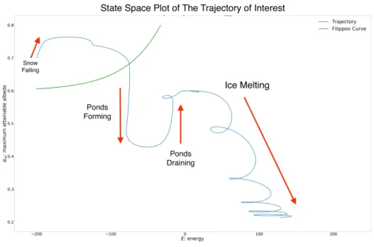
2.1 The state space trajectory that we use in data assimilation experiments. . . 17

2.2 Trajectories with various initial points whenFCO2 = 0. . . 18

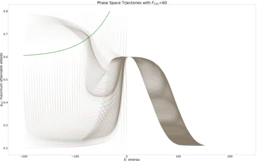
2.3 Trajectories with various initial points whenFCO2 = 60. . . 19

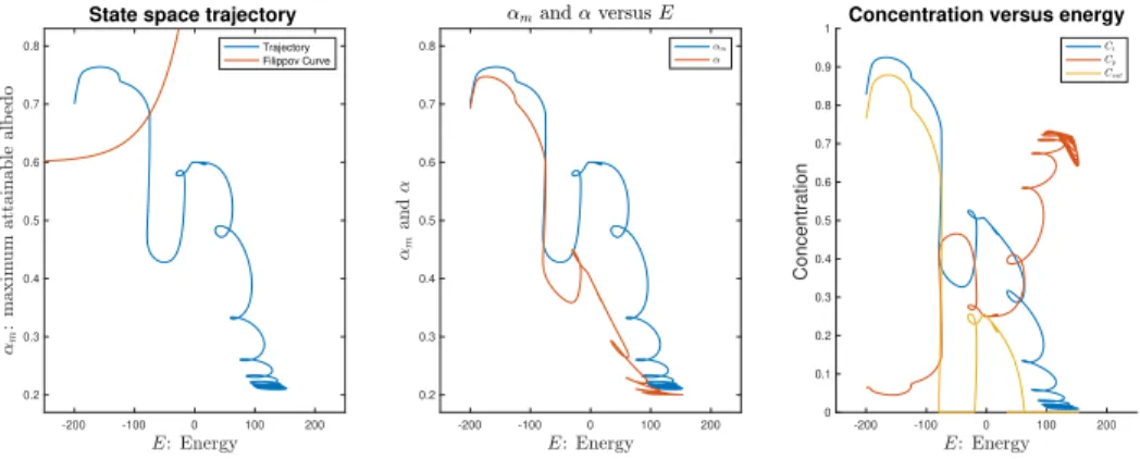
2.4 Overview of the proposed proxy for the melt pond problem in sea ice concentration retrieval. . . 20

2.5 Overview of the proposed proxy for the melt pond problem in sea ice concentration retrieval. . . 21

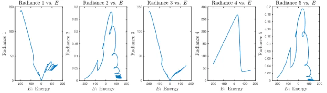
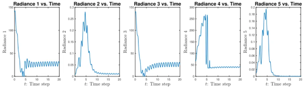
2.6 The proxy for satellite radiances versus energy. . . 21

2.7 The proxy for satellite radiances versus time. . . 22

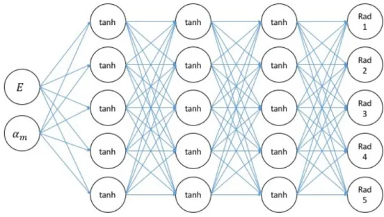
3.1 Graphical representation of the proposed machine learning model. . . 27

3.2 The performance of machine learning observation operator evaluated on one trajectory. . . 28

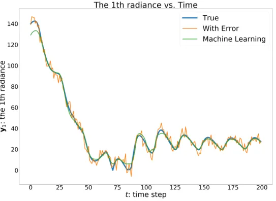
3.3 Time evaluation of the 1st radiance, true value, noisy value and ML fitted value. . . 29

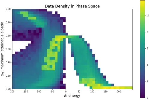
3.4 Density of available training data for machine learning in the state space. . . 30

3.5 Error of machine learning algorithm in state space. . . 31

3.6 Drop out data in the shaded region of interest. . . 33

3.7 Comparison between the original data density (left) and the data density after dropping95%data inE∈[−50,50]. . . 33

3.8 Comparison between the error of machine learning algorithm with all data (left) and with5%data inE ∈[−50,50]. . . 34

4.1 DA experiment withH, the true observation operator. . . 39

4.2 DA experiment withHˆ_ML, i.e. ML OP with grid training data. . . 39

4.3 DA experiment withH_ML, i.e. ML OP with training data from trajectories. . . 40

4.4 DA experiment withHretrieval, the observation operator representing the proxy for satellite retrieval algorithm. . . 41

4.5 DA experiment withH_30%, i.e. ML OP trained with30%data inE∈[−50,50]. . . 42

(8)

4.7 Time evolution of absolute error ofαmwithH,HˆML,HML, andHretrieval, respectively 43

4.8 Time evolution of absolute error ofEwithH,Hˆ_ML,H_ML, andH_retrieval, respectively 43

4.9 Time evolution of absolute error ofαmwithH,HˆML, andHML, respectively . . . 44

(9)

LIST OF ABBREVIATIONS

DA Data Assimilation

EnKF Ensemble Kalman Filter

EW09 The Sea Ice Model Proposed by Eisenman and Wettlaufer in 2009

FNN Fully Connected Neural Network

i.i.d Independent and identically distributed

KF Kalman Filter

ML Machine Learning

NN Neural Network

OP Observation Operator

(10)

LIST OF SYMBOLS

α Albedo, the percentage of solar radiation reflected back

αm Maximum attainable albedo

C(Rn,Rm)Continuous function fromRntoRm

The uncertainty in model

η The uncertainty in observation operator

H Observation operator

H The linearization or matrix form ofH

HML Machine learning observation operator with realistic training data

ˆ

HML Benchmark machine learning observation operator with unrealistically large amount of training data

Hretrieval Observation operator representing the proxy for satellite retrieval algorithm

H_5% Machine learning observation operator with5%data inE ∈[−50,50]for training.

H_30% Machine learning observation operator with30%data inE∈[−50,50]for training.

In The identity mapping inC(Rn,Rn)

K The Kalman gain matrix

M The dynamic model used in data assimilation

M The linearization or matrix form ofM

N(µ,σ) Normal distribution with meanµand error covariance matrixσ.

P The covariance matrix representing the uncertainty in state estimate

Q The covariance matrix representing the uncertainty in model

R The covariance matrix representing the uncertainty in observation

ξ The error of machine learning observation operator.

x The state vector, in our study is2-dimensional containingE andαm.

xf The forecast estimate of the state.

xfi _{The forecast estimate of the}_{i-th ensemble member.}

xa The analysis estimate of the state.

y The observation vector, in our study is5-dimensional representing the satellite radiances.

(11)

CHAPTER 1

Introduction

1.1 Data Assimilation

Data assimilation is an analysis technique in which the observed information is accumulated into

the model state by taking advantage of consistency constraints with laws of time evolution and

physical properties. In this study, we will focus on sequential data assimilation with its discrete time

formulation.

We first consider themodelthat evolves the state variablesxt∈Rnin time, which is typically a dynamical system defined by the mapM ∈C(Rn×N,Rn)

xt+1 =M(xt, t) +t, t∈N (1.1)

where = {t}t∈N is an i.i.d. sequence. In many applications, models are supplemented by

observations of the system as it evolves; this information then changes the probability distribution

on the states, typically reducing the uncertainty. To describe such situations, we assume that we are

given data, or observations,y_t∈Rmdefined as follows. At each discrete time instance, we observe a (possibly nonlinear, as in this study) function of the state variables, with additive noise:

y_t=H(xt) +ηt, t∈N (1.2)

whereη ={ηt}t∈Nis an i.i.d. sequence. The functionHis known as theobservation operator.

The objective ofdata assimilationis to determine information about the statesxt, given datayt, at

each time stept. For example, if we are directly observing all the state variables, then the observation

(12)

variables, then the observation operator becomes a projection. As later described in Section 2.3, the

observation operator in our study is much more complicated and non-linear.

Sequential DA consists of two steps at each discrete time, the prediction step, where the estimate

from last time step is evolved using the model to give theforecast, and the update step, where the

forecast is updated to theanalysisreflecting the observations.

As described above, the observation operator is very important - it allows us to compare our

forecast model states with measurements and obtain a more accurate estimate of the model state.

Passive microwave satellite data is an example where the physical state of a system, ocean temperature,

for example, is not directly observed, but the intensity of microwave radiation it emits is. In a situation

like this, we have two choices for an observation operator.

1. Infer the physical quantities from the light intensities with an inverse scheme. (Often done,

but can be inaccurate) and use an observation operator which is a projection on to the inferred

state variables.

2. Use an observation operator which maps the model state variable directly to the actually

observed quantities.

In cases where the inversion option 1 is not a good choice as incorrect data would be assimilated

pushing the model in the wrong direction. In this situation, it is advantageous to use option 2.

However, option 2 presents its own difficulties,Hmay be highly nonlinear and complex, as is the

case for satellite radiance measurements. In this work, we explore methods for discoveringHusing

data and machine learning with a focus on sea ice modeling.

1.1.1 Kalman Filter

From the beginning of data assimilation, many algorithms that aim to produce the optimal state

estimate under various constraints and assumptions have been proposed. Some popular methods

include 3D-Var, 4D-Var, particle filter, and Kalman filter along with its variants. In this study, we

focus on the Ensemble Kalman Filter. First, let us review the Kalman filter. Named after Rudolf E.

Kalman, the Kalman filter first emerged in control theory. It uses a system’s dynamic model (e.g.,

physical laws of motion), known control inputs to that system, and multiple sequential observations,

(13)

by using only one measurement alone. In terms of data assimilation, the standard Kalman filter

(KF) is the optimal sequential data assimilation method for linear dynamics and observations with

Gaussian error, i.e., we assume in Equation (1.1) and Equation (1.2)MandHare linear mappings

andtandηtat each time step are normal distribution with zero mean. Usually, the problem which

KF applies to can be formulated as follows:

• xb_, _B_{, prior guess of initial state vector and error covariance matrix}

• xt+1=M(xt) +t, t∼ N(0,Qt), whereMis the dynamic model that evolves the state in time andQtis the error covariance matrix for the model. In addition, we have to know the

matrix form (linearization in the case of nonlinear dynamics) ofM:M.

• y_t =H(xt) +ηt, ηt ∼ N(0,Rt), whereHis the observation operator that maps system states to observations, and Rt is the error covariance matrix for the observation operator.

Similarly, the matrix form (linearization in the case of nonlinear observation operator) ofH:

H.

The algorithm goes as follows:

1. Setxa₀ =xbandPa₀ =B

2. Forecast step:

• Propagate the prior guess forward in time,xf_t₊₁ =M(xa_t)

• Propagate the prior guess error covariance matrix forward in time:Pf_t₊₁=MPa_tMT +Q

3. Analysis step:

• Calculate the Kalman gain matrix:K=PfHT(R+HPfHT)−1

• Get the analysis of the state using the observations:xa=xf+K(y− H(xf)

• Calculate the analysis error covariance matrix:Pa= (I−KH)Pf

(14)

1.1.2 Ensemble Kalman Filter

As stated above, the standard Kalman filter (KF) only gives the optimal state estimate for linear

dynamics and measurement processes with Gaussian error statistics. For non-linear situations,

the extended Kalman filter (EKF) can be used with the linearization ofMandH, although it is

well known that EKF is unstable under strong nonlinearities. Both the KF and the EKF explicitly

propagate error information with a dynamic equation for the state error covariance matrix. However,

the integration of this equation is not computationally feasible for large-scale environmental systems.

To overcome these limitations, the ensemble Kalman filter (EnKF) was proposed by (Evensen, 2003).

The ensemble Kalman filter is a suboptimal estimator, where the error statistics are predicted by

using a Monte Carlo or ensemble integration to solve the Fokker-Planck equation. In this study,

we use the formulation of (Gillijns et al., 2006). Like the Kalman filter, EnKF also consists of the

forecast step and the analysis step.

First, to represent the error statistics in the forecast step, we assume that at timet, we have an

ensemble ofqforecasted state estimates with random sample errors. We denote this ensemble as

Xf_t ∈_Rn×q_{, where}

Xf_t = (xf1

t , ...,x fq

t ) (1.3)

and the superscriptfi refers to the i-th forecast ensemble member. Then, the ensemble mean

¯

xf_t ∈Rnis defined by

¯

xf_t = 1

q q

X

i=1

xfi

t (1.4)

From the ensemble members, we calculate the forecast output and the forecast output mean

yfi

t =H(x fi

t ) (1.5)

¯

yf_t = 1

q q

X

i=1

yfi

t (1.6)

We define the ensemble error matrixEf_t ∈Rn×qaround the ensemble mean by

Ef_t = (xf1

t −¯x f t, ...,x

fq

t )−¯x f

(15)

and the ensemble of output errorEfyt ∈R

n×q

Ef_y

t = (y

f1

t −¯y f t, ...,y

fq

t )−¯y f

t (1.8)

The forecast of the error covariance in the state is estimated with the ensemble error covariance, i.e.

Pf_t = 1

q−1E f t(E

f

t)T (1.9)

We also define

Pf_xy

t =

1 q−1E

f t(Efyt)

T _(1.10)

Pf_yy

t =

1 q−1E

f yt(E

f yt)

T _(1.11)

We interpret the forecast ensemble mean¯xf_t as the best forecast estimate of the state, and the sample covariance of the ensemble membersPf_t as the forecast estimate for the uncertainty.

The second step is the analysis step. The Kalman gain matrix is estimated by

Kt=Pfxyt(P

f yyt)

−1 _(1.12)

To obtain the analysis estimates of the state, the EnKF performs an ensemble of parallel data

assimilation cycles, where fori= 1, ..., q

xai

t =x fi

t +Kt(yit− H(x fi

t ) (1.13)

whereyi_tare perturbed observations given by

yi_t=y_t+ηt, ηt∼ N(0,Rt) (1.14)

The ensemble mean and covariance are calculated as follows

¯

xa_t = 1

q q

X

i=1

xai

(16)

Pa_t = 1 q−1E

a

t(Eat)T (1.16)

and are used as the best analysis estimate of the state and uncertainty, respectively. The last step is

the prediction of error statistics in the next forecast step:

xfi

t+1=M(x ai

t ) +t, t∼ N(0,Qt) (1.17)

Unlike the extended Kalman filter, the evaluation of the filter gainKtin the EnKF does not

involve an approximation of the nonlinearity M and H. Hence, the computational burden of

evaluating the Jacobians ofMandHis absent in the EnKF.

As we can see from the formulation of EnKF, it is a sub-optimal estimation derived from Kalman

filter to compensate for high computational cost and nonlinearity. Like the Kalman filter, EnKF

would still perform better under the same constraints and assumptions of Kalman filter. Typically,

the closer the actual system is to linear and Gaussian, the more likely EnKF is useful.

However, when there is a systematic error or bias in our knowledge about the observation

operatorH, wrong information might be assimilated into the system and the analysis could be even

worse than the forecast. If the true observation operator isH, but we think it is insteadH0_{, when}

calculating the output forecastyfi

t in Equation (1.1.2), we would useH0 instead of the correctH. Intuitively, even if the forecast ensemble statesxfi

t are exactly the same as the truth, forecast output

of the ensemble membersyfi

t =H0(x fi

t )would be far from the observation which is generated by

Hinstead ofH0, and the update step based on such difference would likely drive the model farther

away from the truth. Since the calculation of the Kalman gain matrix Equation (1.12) is based on the

output forecast through Equation (1.1.2) and Equation (1.1.2), the algorithm would likely to give an

estimate of the Kalman gain matrix that is far from the truth. Furthermore, in Equation (1.13), each

ensemble member is updated with the Kalman gain and the difference between the observation and

forecast output, where we again would put the wrongH0_{in the equation. In our study, this is exactly}

what happens in a sea ice concentration retrieval algorithm when melt ponds obscure the microwave

(17)

1.2 Sea Ice Modeling and Data Assimilation

1.2.1 Numerical Sea Ice Models

A complete sea ice model consists of a momentum equation, thermodynamic model, and an equation

governing the evolution of the ice thickness distribution. Here we give a brief review of the standard

equations used to model sea ice on large scales (Hunke et al., 2017). The typical form of the

momentum equation for sea ice is given by,

ρ¯hdv

dt =∇ ·(¯hσ) +τa+τw−fc−ρ¯hga∇H. (1.18)

Herevis the ice velocity,σ the stress,τa atmospheric forcing,τw ocean forcing,fcthe Coriolis

force,Ha sea surface tilt term,ρthe ice density,¯hthe average ice thickness, andgagravitational acceleration. In addition to a thermodynamic model, the ice thickness distribution,g, are tracked and

evolved according to the ice thickness distribution equation (Thorndike et al., 1975) given by,

dg

dt + (∇ ·v)g+ (f g)

h =ψ. (1.19)

The first two terms in equation 1.19 describe horizontal transport and the changes in ice

thick-nesses due to flow,f =dh/dtis the rate that thickness changes due to thermodynamic processes andψa term accounting for mechanical redistribution due to ridging, where convergence causes ice

to pile up. Typically discrete thickness categories are tracked within a grid cell of the model and

measures of observable quantities, such as ice concentration, can be calculated by looking at the

amount of ice in the zero thickness categories. In this work, we focus on sea ice concentration as a

quantity of interest for assimilation into a large scale sea ice model.

1.2.2 Sea Ice Concentration Retrieval

Sea ice concentrations themselves are derived by exploiting the high contrast in the microwave

emissivities of sea ice and open water. The satellite itself retrieves the brightness temperatureTB.

The brightness temperature can be approximated, in the microwave regime, through the dimensionless

(18)

with the equation

TB(λ, p) =εs(λ, p)Ts. (1.20)

Hereλis the wavelength,pthe polarization, andTsis the physical temperature in degrees Kelvin.

The emissivity itself depends on the dielectric properties of the emitting material. For sea ice, this

is primarily a function of the salinity and brine volume fraction while for snow it is the grain size

and water content. Further, the atmosphere must also be considered since the brightness temperature

retrieved by the satellite is a combination of several contributions from the Earth, atmosphere, and

space.

Once atmospheric and other effects are accounted for, the retrieved brightness temperature can

be thought of as coming from a mix of open water, first year, and multiyear sea ice. The assumption

is that the measured temperature brightness is coming from a linear mix of the constituents. That is,

withFbeing the fraction,

TB(λ, p) =εs(λ, p)Ts=εw(λ, p)TwFw+εf y(λ, p)Tf yFf y+εmyTmy(λ, p)Fmy (1.21)

wheres,w,my,f ystand for the scene, water, multiyear and first-year ice respectively.

For many of the established algorithms, retrieval of ice concentration depends on tie points which

are observed brightness temperatures for open waterTBw, first-year iceTBf y, and multiyear ice

TBmy. The tie points themselves incorporate most atmospheric effects and can depend on location,

the season, and the sensor itself. The successful retrieval of ice concentration relies heavily on having

correct tie points. In the wintertime, these do not vary much. However, in the summer, observed

brightness temperatures can vary greatly both spatially and temporally (Willmes et al., 2014).

As the melt season progresses, higher water content in the snow layer atop the ice increases the

microwave emissivity of the snow while absorbing most of the emissions from the ice below. The

snow itself can have an emissivity close to 1 compared to that of multiyear ice at 0.7-0.8 or first-year

ice at 0.9-0.95. This can have the effect of increasing the overall emissivity of a given scene. As the

snow melt progresses, water runoff settles into the topographic low points of the surface forming melt

ponds. These ponds continue to grow, deepen and eventually connect to form complex geometries

(19)

when the ice becomes sufficiently permeable. Melt ponds have a microwave signature very close

to that of open water at the relevant frequencies and also absorb most of the emission from the ice

below. This has the opposite effect of wet snow, decreasing the overall emissivity. The increased

emissivity of the wet snow is likely to push toward a concentration retrieval on the high side, whereas

melt ponds tend to push toward lower values (Kern et al., 2016; Kongoli et al., 2011). The extent

of these effects on sea ice concentration retrieval depends on the tie points of the algorithm used.

Many algorithms are tuned to mitigate the masking effect of melt ponds in the summer to provide

concentrations that more closely represent the extent of sea ice. These values are important for heat

fluxes as the heat flux of sea ice and the ocean differs significantly.

One might also be interested in albedo. In this case, one would want a concentration that more

closely represents the surface fraction of exposed sea ice. This is because the critical factor here is

the difference between the albedo of melt ponds and the ice. For this purpose, one may not want to

mitigate the masking effect of melt ponds at all. As an example, in (Kern et al., 2016) it was observed

that for100%sea ice concentration with40%melt pond coverage, many of the standard concentration retrieval algorithms returned concentrations of≈90%. While still an underestimation, this value is a far cry from the 60% sea ice surface fraction an algorithm not tuned to account for melt ponds

might produce. Further, for an algorithm that is tuned high, the large spatial and temporal variability

of surface conditions in summer can lead to concentration retrievals of>100%. In addition, ponds can rapidly drain through the porous microstructure of the ice when it is warm enough, this means a

retrieval algorithm tuned high will be over predicting concentrations in situations where ponds have

disappeared.

Attempts to quantify this effect were carried out in (Kern et al., 2016). Linear correlations were

found in a comparison of sea ice concentrations obtained using NASA’s MODIS sensor, which can

resolve melt ponds, and NASA’s AMSR-E sensor. The slopes ranged from 0.9 to 1.12 , depending

on the algorithm, indicating that some algorithms are underestimating concentration while others

are overestimating it. These errors have been found to be as high at26%when compared to data obtained using NASA’s Moderate Resolution Imaging Spectroradiometer (MODIS) sensor (Kern

et al., 2016). This can create serious problems when attempting to assimilate concentration data into

large scale sea ice models. Many large scale sea ice models also include pond fraction as a state

(20)

the true values, one would not want to assimilate a retrieved concentration of 70% ice, the amount

hidden by the ponds.

1.2.3 Assimilating with the satellite radiances

Given that 100% ice and 30% ponds looks the same to a passive microwave satellite as 70% ice and

no ponds, in that observed radiances are very similar, one possible way to avoid the assimilation of

incorrect data is to change the observation operator and map the state variables of the model to the

radiances instead of obtaining an (inaccurate) estimate of state variables from them. This itself is

a challenging task and the radiances emitted by a scene of emissivity will depend not only on the

fraction of ice, water, and ponds, but on the thickness, salinity, temperature and snow cover of the ice.

Perhaps the most difficult parameter to estimate is sea ice emissivity. Sea ice may be viewed as a

composite of ice and brine, and the microwave emissivity depends heavily on the volume fraction and

configuration of the brine pore space, a problem which relates to classic problems in homogenization

theory. Further atmospheric effects need to be taken into consideration as it serves as an intermediate

layer between the ice pack and observing satellite.

One method previously studied uses various parameterizations of sea ice emissivities and an

atmospheric radiative transfer model to build a complex observation operator which takes sea ice

model state variables directly to passive microwave satellite radiances (Scott et al., 2012). It was

found that this improved model predictions, especially during the melt season. However, it is sensitive

to the parameterization of emissivity chosen and computationally expensive. In this work a 3D-var

assimilation scheme was used. However, the Ensemble Kalman Filter (EnKF) has many advantages

over 3D-Var but due to the needed atmospheric modeling would be computationally prohibitive. We

instead propose to use a machine-learned observation operator which takes inputs of sea ice state

variables and rough atmospheric conditions and outputs likely observed satellite radiances. Once

learned, the low computational cost of the observation operator would allow for an EnKF scheme

to be possible. The primary difficulty here, however, is in building a data set to train on. As a first

step, we will use a simple Testbed Model designed to mimic how ponds form and drain during the

melt season with proxies for satellite radiance, true ice concentration, pond fraction, and retrieved

concentrations to investigate how successful a machine learning observation operator is in improving

(21)

1.3 Machine Learning

Machine learning (ML) is the scientific study of algorithms and statistical models that computer

systems use to effectively perform a specific task without using explicit instructions, relying on

patterns and inference instead. It is seen as a subfield of artificial intelligence. Machine learning

algorithms build a mathematical model of sample data, known as “training data”, in order to make

predictions or decisions without being explicitly programmed to perform the task. Machine learning

algorithms are used in a wide variety of applications, such as email filtering, and computer vision,

where it is infeasible to develop an algorithm of specific instructions for performing the task. Machine

learning is closely related to computational statistics, which focuses on making predictions using

computers. The study of mathematical optimization delivers methods, theory and application domains

to the field of machine learning.

1.3.1 Neural Networks

Neural networks (NNs) are computing systems vaguely inspired by the biological neural networks

that constitute animal brains. The neural network itself is not an algorithm, but rather a framework for

many different machine learning algorithms to work together and process complex data inputs. Such

systems “learn” to perform tasks by considering examples, generally without being programmed

with any task-specific rules.

An ANN is a model based on a collection of connected units or nodes called artificial neurons,

which loosely model the neurons in a biological brain. Each connection, like the synapses in a

biological brain, can transmit information, a “signal”, from one artificial neuron to another. An

artificial neuron that receives a signal can process it and then signal additional artificial neurons

connected to it. In common ANN implementations, the signal at a connection between artificial

neurons is a real number, and the output of each artificial neuron is computed by some non-linear

function of the sum of its inputs. Artificial neurons and edges typically have a weight that adjusts

as learning proceeds. The weight increases or decreases the strength of the signal at a connection.

Typically, artificial neurons are aggregated into layers. Different layers may perform different kinds

of transformations on their inputs. Signals travel from the first layer (the input layer) to the last layer

(22)

the neural network can be summarized as

xl+1=fl(Wlxl+bl) (1.22)

whereflis a element-wise nonlinear function called the “activation function”. We may have different

activation functions for different purposes in different layers. For example, in our study, the hidden

layers all havetanhas the activation function while the final output layer does not have activation function, i.e.,foutis the identity mapping.

1.4 Rationale for Testbed Model

As mentioned in Section 1.2.3, the motivation of this study is to investigate how successful a machine

learning observation operator is in improving predictions compared to retrieved concentrations.

Typically, sea ice dynamics are simulated with the numerical sea ice models described in Section 1.2.1

e.g., the Community Sea Ice Model (CSIM) (Hunke and Lipscomb, 2010). However, use of such

large-scale sea ice models in this study, while describable, would act as a bottleneck preventing

timely exploration of the state space and its relationship to satellite radiance values. This is partly

because of the computational cost in running the large-scale models, especially in EnKF, where a

large ensemble is needed, and the dynamics of every ensemble member needs to be calculated. Also,

the state space in a large-scale sea ice model is usually high-dimensional. Here we wish to be able to

fully explore the state space, and so we will require a low-dimensional model.

Besides a low-dimensional model, we also need to define proxies for satellite radiances, ice

concentration, and pond concentration from the model state variables. While real observations

exist, for this initial study, we focus on exploring how machine learning can be used to discover

an observation operator. Therefore we desire to have complete control over the state variables, the

observations, and the error in each and as such real ice observations would not be appropriate for use

at present.

In data assimilation, Lorenz’96 (Lorenz, 1995) is often used as a model problem. It is a 40-dimensional dynamical system formulated by Edward Lorenz in 1996, originally used to study issues

(23)

success with Lorenz’96. However, it is not sufficient to make our argument. In this work, we are

motivated by the sea ice concentration retrieval problem caused by melt ponds, so we seek a low

dimensional model which mimics the specific situation of interest. For example, the formation and

drainage of ponds cause errors in retrieved concentrations which would not otherwise be present, and

the model should display behaviors representing such phenomenon.

To this end, we use the ODE energy balance model of (Eisenman and Wettlaufer, 2009). This

model accounts for energy input and loss in sea ice and as a result, can give us an accounting of

how and when a pond should form or drain. However, this model does not explicitly have a variable

related to the formation of melt ponds. Therefore, we will introduce a second ODE and variable to

account for this. Since we will only have two variables, we will be able to easily explore the whole

state space by simply generating model runs of different initial conditions. This will further allow us

to create a proxy for satellite radiances, ice concentration, and pond fraction based on a simple input

space. The details of this model are presented in Chapter 2. With this model, we are able to focus on

(24)

CHAPTER 2

Testbed Model Formulation

2.1 Original Model of Eisenman and Wettlaufer

As mentioned in Section 1.2.3, we build a Testbed Model to mimic the physical process of ponds

forming and draining form to investigate how successful a machine learning observation operator

is in improving predictions compared to retrieved concentrations. We base our model on a simple

sea ice model developed by I. Eisenman and J.S. Wettlaufer in 2009 (EW09). The original ODE of

(Eisenman and Wettlaufer, 2009) is given by:

dE

dt = [1−α(E, αm)]Fs(t)−F0(t) +Fco2 −FT(t)

E cmlHml

+FB (2.1)

where α(E, αm) =

αml+αm 2 +

αml−αm 2 tanh

E Lihc

(2.2)

In Equation (2.1), Fs(t) is the incoming solar radiation, F0(t) is the amount of longwave radiation(heat) that escapes to space,FCO2 is the amount of longwave radiation reflected back from

clouds and CO2,FT(t)has to do with heat exchange with lower latitudes, andFBis the heat input from the ocean below the ice. In the original model,FCO2 andFBare constants, whileFs(t),F0(t), andFT(t)are taken to be step-wise constant functions consisting of the monthly averaged values. In our study, the time-dependent quantities are replaced with continuous functions consisting of10-term Fourier series fitted to the monthly averaged values. Meanwhile, we are most interested inFCO2, and

we will vary its value to investigate its influence on the system.

In the model, Equation (2.2) represents the albedo (the percent of incoming solar radiation the

ice reflects) and depends on the energy of the ice as a whole. In this equationαml is the albedo

(25)

thickness which is used to control the smoothness of the parameterization. In the original model,

αm is the maximum attainable albedo of the ice which they take to be0.68. In reality, it can be as high as0.8with snow on top of it in cold conditions. AsEincreasesαgoes down, this serves as a way to account for the ice albedo feedback caused by the formation of melt ponds. However, this

does not take into account pond drainage. As sea ice warms, it becomes increasingly permeable to

fluid flow. Large connected pathways form in the ice called brine channels. When these connect up

enough, ponds can drain through the porous microstructure of the ice into the ocean. This happens

at temperatures higher than when the ponds initially form. With the dark-colored ponds removed,

the albedo of the ice is temporally increased and more solar radiation reflected. In this work, we are

interested in having a model which mimics, in some way, ponding on sea ice. To approximate this

behavior, we will allow the maximum attainable albedo to vary withEin a way that roughly mimics

the effect of pond drainage. We will also use the values ofE andαm to ”measure” pond and ice

fractions. This is discussed below.

2.2 Proposed Model

The primary argument for makingαmchange in time will be the following, in very cold conditions

the maximum attainable albedo of the surface should tend toward 0.8 with snow fall and other processes keeping the albedo high. When the ice is in warmer conditions, like melting, the maximum

attainable albedo should tend to lower values, e.g. 0.2, the albedo of open water, and there should be a competition of values. Initially, as the ice begins to pond the albedo drives down pretty quickly,

however as the ice temperature increases the ice becomes permeable and the melt ponds drain out,

which then causes the albedo of the ice to recover quickly. In order to mimic this physical process, we

model the rates of change of the maximum attainable albedoαmwith a Filippov system (F. Filippov,

(26)

dE

E cmlHml

+FB dαm

dt = E2 K₁2αm

1−αm

0.8

+ K 2 2 1 +E2αm

1− αm

0.6

in S1 ={(E, αm) :H(E, αm)>0} (2.3)

dE

E cmlHml

+FB

dαm dt =

K₃2 1 +E2αm

1−αm

0.6 + E 2 K2 4 αm

1− αm

0.2

in S2 ={(E, αm) :H(E, αm)<0} (2.4)

where H(E, αm) =α(E, αm)−0.6. (2.5)

In our proposed model, the dynamics for the energy E is the same as the original EW09

model. αm is modeled by separate equations representing the two different situations. In “cold”

conditions,αmis modeled by competing logistic models with the carrying capacity to be0.8and0.6 Equation (2.3). In “warm” conditions,αmis similarly modeled by competing models with carrying

capacities of0.2and0.6Equation (2.4). We also let the growth or decay rate in these equations depend on the energyEand some scaling factorKi’s. The two parts of the dynamics are separated

by the discontinuity boundaryH = 0, whereH is defined by the smooth function Equation (2.5). Since the boundary is supposed to divide the state space into “cold” and “warm” parts, therefore

we choose the boundaryH = 0to simply be where the albedo of the systemα(E, αm)crosses the α= 0.6threshold. Figure 2.2 is a plot of a state space trajectory of the system, with initial condition E = −200, αm = 0.7and parameter valueFCO2 = 60. It gives an example of how the system

behaves.

• In cold conditions, the system is at the left top part of the state space shown in Figure 2.2,

whereα(E, αm) > 0.6. When the energy is largely negative, the logistic model term with the energy in the numerator dominates in Equation (2.3), and the maximum attainable albedo

(27)

Figure 2.1: The state space trajectory that we use in data assimilation experiments.

falling. The initial rise from0.7towards0.8in Figure 2.2 illustrates to this process. When the energy is close to zero, the term with the energy in the denominator (with the addition of 1 to

avoid singularities atE = 0) dominates, andαmapproaches0.6, which is not apparent from Figure 2.2. As the system’s energy keeps increasing, it crosses the boundary between the two

parts of dynamics.

• In warm conditions, the system is at the center part of the state space shown in Figure 2.2,

whereα(E, αm) <0.6. The rate thatαm approaches0.2is faster when the energy is away from0whereas the rate to approach0.6is faster when the energy is near0. As a result, we take the energy to be in the denominator for the logistic model with a carrying capacity of

0.6and the energy in the numerator for the logistic model with a carrying capacity of0.2 Equation (2.4). In Figure 2.2, we can see that right after the system crosses the boundary,αm

is rapidly driven towards0.2, representing the process of ponding. When energy is higher, the ice becomes permeable, and melt pond drainage exposes the surface of the ice again, causing

(28)

Figure 2.2: Trajectories with various initial points whenFCO2 = 0.

Figure 2.2 and Figure 2.2 plot the boundary curve and trajectories from various initial points

in the state space with different values of FCO2, respectively. When the value ofFCO2 is small,

as in Figure 2.2 whereFCO2 = 0, the energy of the system stays negative, whereas whenFCO2

is sufficiently large, as in Figure 2.2 whereFCO2 = 60, the states that start with negative energy

will cross zero and become positive. In our data assimilation experiments, we will focus on one

particular trajectory of interest, the one with initial conditionE=−200,αm = 0.7and parameter valueFCO2 = 60. The aforementioned Figure 2.2 plots this trajectory along with the boundary curve

separating the two parts of the dynamical system.

In terms of discrete time sequential data assimilation, the state variable is a two dimensional

vector defined by

x= (E, αm) (2.6)

The model Min Equation (1.1) is therefore defined by integrating the ODE Equation (2.3) or

Equation (2.4) in time

M(xt, t) =

Z (t+1)∆τ

t∆τ

dx

(29)

Figure 2.3: Trajectories with various initial points whenFCO2 = 60.

where d_dtx = (dE_dt,dαm

dt ), and∆τ is the time step in data assimilation. In our study, all the ODE’s are numerically integrated using the Matlab programdisode45(Calvo et al., 2016) with its default

settings (the major algorithm parameters include absolute error tolerance10−6 and relative error tolerance10−4).

2.3 Proxy for Ice and Pond Concentration and Satellite Radiances

As mentioned in Section 1.2.3, for our particular problem, we need to define from our state variables

E andαm proxies for other physical quantities of interest, including ice and pond concentration

values, the satellite radiances, and satellite-retrieved ice concentration. In Equation (2.8) We define

the concentration of iceCito be the one minus the percent difference between the physically highest

attainable albedo of0.8and the average of the maximum attainable albedo and the current albedo. The concentration here would approach 1 when the system is in a very cold state and the average is

(30)

-200 -100 0 100 200 0.2 0.3 0.4 0.5 0.6 0.7 0.8

State space trajectory

Trajectory Filippov Curve

-200 -100 0 100 200

0.2 0.3 0.4 0.5 0.6 0.7 0.8

-200 -100 0 100 200

0 0.1 0.2 0.3 0.4 0.5 0.6 0.7 0.8 0.9 1 Concentration

Concentration versus energy

Figure 2.4: Overview of the proposed proxy for the melt pond problem in sea ice concentration retrieval.

Ci(E, αm) = 1−

0.8−1₂(αm+α(E, αm)) 0.6

!

(2.8)

The pond concentration is defined as one minus the ratio of the current albedo to the maximum

surface albedo. The idea here is that a low albedo at timetcompared to the maximum attainable

albedo should mean the surface is covered in ponds.

Cp(E, αm) = (0.5 tanh(

E+ 200

10 ) + 0.5)(1− 0.2 α(E, αm)

)1000(1−αm

0.8) (2.9)

For the satellite retrieved concentration, to model the fact that the melt ponds obscure the

microwave signature of the ice and thus melt ponds and open water are indistinguishable in terms of

satellite radiances as mentioned in Section 1.2.2, we take the maximum of zero and the difference

between ice concentration and pond concentration.

Csat(E, αm) = max(0, Ci(E, αm)−Cp(E, αm)) (2.10)

Figure 2.3 plots the quantities of interest as they change with the state variables on the trajectory

shown in Figure 2.2 in the state space. Figure 2.3 gives plots of the time evolution of quantities of

interest.

Finally, for the satellite radiances, we define functions of the state variables that give non-unique

(31)

0 5 10 15 20 -200 -150 -100 -50 0 50 100 150 200

0 5 10 15 20

0.2 0.3 0.4 0.5 0.6 0.7 0.8

0 5 10 15 20

0 0.1 0.2 0.3 0.4 0.5 0.6 0.7 0.8 0.9 1

Figure 2.5: Overview of the proposed proxy for the melt pond problem in sea ice concentration retrieval.

-200 -100 0 100 200

0 50 100 150

-200 -100 0 100 200

0 0.05 0.1 0.15 0.2 0.25 0.3

-200 -100 0 100 200

0 50 100 150

-200 -100 0 100 200

0 50 100 150 200 250 300

-200 -100 0 100 200

0 0.02 0.04 0.06 0.08 0.1 0.12 0.14 0.16 0.18 0.2

Figure 2.6: The proxy for satellite radiances versus energy.

change with the state variables on the trajectory shown in Figure 2.2 in the state space. Figure 2.3

gives plots of the time evolution of the five radiances.

O(E, αm) =

           

|Eαm|

αm−α(E, αm) α(E, αm)|E|

(0.5 + 0.4 tanh(50₁₀−E))(E+ 273.15) Ci(1−α(E,α_α_mm))

            (2.11)

2.4 Problem of Using Satellite Retrived Concentration in DA

In terms of data assimilation, if we assimilate with the satellite retrieved concentration, the real

(32)

0 5 10 15 20 0

50 100 150

Radiance 1 vs. Time

0 5 10 15 20 0 0.05 0.1 0.15 0.2 0.25 0.3

0 5 10 15 20 0

50 100 150

0 5 10 15 20 0 50 100 150 200 250 300

0 5 10 15 20 0 0.02 0.04 0.06 0.08 0.1 0.12 0.14 0.16 0.18 0.2

Figure 2.7: The proxy for satellite radiances versus time.

be the actual satellite retrieved ice concentrationCsat as a function ofEandαmin Equation (2.10)

H_sat(x) =H_sat(E, αm) =Csat(E, αm) = max(0, Ci(E, αm)−Cp(E, αm)) (2.12)

However, since we think it is supposed to give the correct ice concentration, the observation operator

Hretrievalthat is used to produce forecast outputyfti in Equation (1.1.2) and Equation (1.13) would be

the ice concentrationCi(E, αm)as a function ofEandαm in Equation (2.8)

H_retrieval(x) =Ci(E, αm) = 1−

0.8−1₂(αm+α(E, αm)) 0.6

!

(2.13)

In this case, there is a systematic bias betweenH_sat andH_retrieval. As discussed in Section 1.1.2, the apparent error in our knowledge about the observation operatorHcould create severe problems

in EnKF, and thus assimilate wrong information into our state estimate. Therefore, we propose to

assimilate directly on satellite radiances with machine learned observation operator. In that case, our

observation space is no longer the1-dimensional space of ice concentration, but the5-dimensional space of the satellite radiances. The real observation operatorHwould be

H(x) =H(E, αm) =O(E, αm) =

           

|Eαm|

αm−α(E, αm) α(E, αm)|E|

(0.5 + 0.4 tanh(50₁₀−E))(E+ 273.15) Ci(1− α(E,α_α_mm))

(33)

While we do not have information of the specific form of the five functions in Equation (2.14)

that make upH, we aim to find with machine learning a functionH_ML ∈C(R2,R5)that closely approximatesH, that is

H_ML≈ H or H(xt, t)− HML(xt, t) =ξt (2.15)

whereξtis ideally an i.i.d sequence with0mean and small variance. In this way, although there is still an error betweenHMLandH, the systematic bias present in the case ofHsatandHretrievalis gone.

Ifξtdoes behave like an i.i.d sequence with0mean and small variance, we can incorporate this error as part of the uncertaintytin the forecast model in Equation (1.1) or as part of the uncertaintyηtin

the observation in Equation (1.2).

• In Equation (1.1.2), HML would be used to calculate {yfti} i=q

i=1, which are further used to

estimate the Kalman gain. Without explicitly quantifying the error in the approximation of

HMLtoH, we could think of this error as coming from the ensemble states{xfti} i=q

i=1instead

of from H_ML, since both uncertainty in {xfi

t } i=q

i=1 and HML could could contribute to the

uncertainty in{yfi

t } i=q

i=1. We will discuss this perspective in more details in Section 4.3.

• Furthermore, in Equation (1.13), each ensemble member is updated with the Kalman gain

and the difference between the observation and forecast output, whereHMLis used in place

ofHin the equation. Here we could consider the uncertainty brought byH_MLas part of the uncertainty in the observationsy_t.

y_t− HML(xfti) =yt− H(xt, t) +ξt=ηt+ξt (2.16)

Originally, the observations are perturbed byN(0,Rt)in Equation (1.14) to account for uncer-tainty. Here we could account for this increased uncertainty fromH_MLby first appropriately

estimatingξtand further perturbing the observations accordingly. This is discussed in more

(34)

CHAPTER 3

Methods

3.1 Data Generation

To generate a data set for the training of machine learning observation operators, we first select points

from the state space asX, calculate the corresponding radiancesY, i.e. observations, and finally add

error to the observations to getY˜.

state space points The first data set we generate isD_traj. To mimic the situation in the real world,

we decide to use points on various trajectories in the phase space to formXtraj. From the model’s

formulation, the maximum attainable albedoαmis only meaningful between0.2and0.8, and the region of interest forE is between−200to0. Therefore,20×30uniform grid data points from S = [−200,0]×[0.2,0.8]are chosen as initial conditions. Figure 2.2 and Figure 2.2 are in fact generated with such initial values withFCO2 = 0andFCO2 = 60, respectively. Note that in our

dynamical system Equation (2.3) and Equation (2.4), the forcing parameterFCO2 is also of interest.

The real world analogy ofFCO2 would be the combined influence of total carbon dioxide emissions,

different weather conditions, climate changes, and etc. Thus we should expect various values of

FCO2 in the data set. To capture this effect, we generate trajectories with12values ofFCO2 ranging

from−10to100. The model is run for200time steps with a step length of0.05for each initial condition and each value ofFCO2, resulting in2400trajectories and1440000data points. From the

data points,Ytraj=H(Xtraj)are calculated and noises are added to giveY˜traj.XtrajandY˜trajform the

data setDtraj= (Xtraj,Y˜traj).

grid data points From Figure 2.2 and Figure 2.2, we can see that in places where the limit cycles

exist, the trajectories are clustered and the data is dense in that region, whereas in places where

(35)

Section 3.3.1, such imbalance creates a problem for the machine learning algorithm. To fully exploit

the potential of the machine learning algorithm to fit the satellite radiances, we also generate a data

set with the unrealistically large amount of data filling up the whole state space.2000×3000uniform grid data points fromS = [−200,0]×[0.2,0.8]are chosen to formXgrid. From the data points,

Ygrid=H(Xgrid)are calculated and noises are added to giveY˜grid.XgridandY˜grid form the data set Dgrid = (Xgrid,Y˜grid).. We expect that with sufficient data, the machine learning algorithm should

perform well everywhere in the state space.

observations and error The observations are calculated for each of the generated data points with

Equation (2.11). In the real world, the data is never perfectly clean, so it is important to add error in

the observations. Moreover, the machine learning algorithms are expected to average out the white

noise error and learn the true pattern behind the noises. Note that the five radiances have different

magnitude scales, radiance 1,3,4 are of∼101_{while radiance 2,5 are of}_∼₁₀−2_{. We initially did} not take such effect into account and add the same errorN(0,1)to all five radiances. Experiments showed that machine learning algorithms were not able to learn anything about radiance 2,5. We also

tried to add error proportional to the value of each radiance at each point. However, this approach

created a problem for values near0, in which case essentially no error is present. Our final approach is adding error proportional to the mean absolute value of each radiance.

¯ yj =

n

X

i=1

|yij| (3.1)

˜

yij =yij +ηij (3.2)

ηij ∼ N(0, λ¯yj) (3.3)

whereλis a control parameter for the magnitude of the error. We generate 7 datasets withλ ∈

{0,0.1,0.2,0.3,0.4,0.5,0.6}to investigate how error affects machine learning algorithms. In data

(36)

3.2 Model Training and Selection

Since we construct the function for satellite radiancesHin a highly nonlinear manner, we decide to

use the artificial neural network (ANN) as the machine learning algorithm. Other algorithms such

as XGBoost and Random Forest are also worth experimenting in the future. We split the data set

randomly into90%for training and validation, and10%for evaluation. We also exclude from the training set the points on the trajectory that we will use in the DA experiment to avoid overfitting. The

training-validation set is further split into the training set and validation set. We choose hyperbolic

tangenttanhas the activation function in hidden layers. We add batch normalization (Ioffe and Szegedy, 2015) before each hidden layer and dropout (Srivastava et al., 2014) after each hidden layer

to regularize the network and prevent it from overfitting. All parameters are initialized using Xavier

initialization (Glorot and Bengio, 2010). The network is trained with Adam optimizer (Kingma

and Ba, 2015). Hyperparameters are chosen based on 9-fold cross-validation. The network is

implemented in Python with Keras framework using Tensorflow as backend. After experiments, we

choose four layers to get our architecture shown in Figure 3.2. The machine learning model can be

written as a composed function in Equation (3.4)

y=xout=W4(tanh(W3(tanh(W2(tanh(W1xin+b1)) +b2)) +b3)) +b4 (3.4)

wheretanhis the element-wise hyperbolic tangent function,W2,W3,W4 are5×5matrices,W1 is a5×2matrix andb1,b2,b3,b4are5-dimensional vectors. The total number of parameters is105. The parameters are determined by the optimization algorithm.

3.3 Evaluation

To examine the accuracy of the prediction model, two evaluation measures are used in this study:

(37)

Figure 3.1: Graphical representation of the proposed machine learning model. as: RMSE= v u u t 1 nm n X i=1 m X j=1

(y_ij0 −yij)2 (3.5)

MAPE= 1 nm n X i=1 m X j=1

y_ij0 −yij yij (3.6)

whereyijis thejth feature of theith sample,yij0 is the predicted value of the correspondingyij.

Figure 3.3 plots the points on the trajectory that we will use in the DA experiment and the

corresponding values of radiance 1,2,4 on those points. Figure 3.3 is a larger illustration of the lower

left plot of Figure 3.3. The figures compare the values given by machine learning algorithmH_ML(X) with the truthYand the noisy training dataY˜ withλ= 0.4. In most places, the machine learning values overlap with the truth and give reasonable values in general. Particularly, it seems that machine

learning is able to average out the noise and discover the real pattern in the data. In the lower middle

plot of the 4th radiance value, even though the noise in the training data is disproportionately large,

our machine learning model is still able to recover the true values behind the noise. In fact, through

experiment, we found out that, with appropriate techniques and sufficient data, machine learning is

(38)

Figure 3.2: The performance of machine learning observation operator evaluated on one trajectory.

machine learning modelHˆMLtrained with a large amount of data is almost perfect, as we expected.

The plot is not shown since the machine learning values virtually overlap with the truth everywhere.

In some sense, we can safely say that the machine learning algorithm fit the function perfectly and

should be identical as and indistinguishable from the true functionH. The accuracy ofH_MLand ˆ

H_MLsatisfies our assumption in Equation (2.15) that the error in the machine learned observation

operator should be white noise with zero mean and small variance.

3.3.1 Data Density

Although in general machine learning achieves a high level of accuracy, H_ML displays different levels of error in different parts in the state space. It is well known that the amount of available

training data is a significant factor in determining the performance of machine learning algorithms.

In our study, since we generate data with trajectories forH_ML, the data points are not uniformly

distributed spatially. In regions where the system achieves equilibrium states and where limit cycles

exist, the data points are clustered together and we therefore have a large amount of data to train

the machine learning algorithm. In regions where the system goes through transient states, the data

points are sparse and we have a limited amount of data to train the machine learning algorithm. The

experiments show correlation between the accuracy and the amount of available training data, or data

(39)

Figure 3.3: Time evaluation of the 1st radiance, true value, noisy value and ML fitted value.

expected error in different regions, we divide the state space into45×30uniform grids, with each grid square representing10units in energyEand0.02unit in maximum attainable albedoαm. In each grid square, we sum up the number of data points in the training data (and then take logarithm)

to represent the data density in this square region. We take the averaged RMSE of all the values in

the grid square to serve as the expected error estimation in that region. Figure 3.3.1 is a heat map

plot of the density in the grid regions, where the color bar represents the logarithm of the number of

available data points in each grid. Figure 3.3.1 is a heat map plot of the expected error in the grid

regions, where the color bar represents the averaged RMSE.

From the plots, we can see the correlation between data density and error. The darker blue colors

in Figure 3.3.1 roughly correspond to the lighter green-yellow colors in Figure 3.3.1. In particular,

for the equilibrium states, where sufficient training data exists, our model tends to perform quite well,

whereas for the transient state, where training data is extremely sparse, the values given by machine

learning does not make much sense. As previously described in Section 2.4 and Equation (2.15), we

expect the difference betweenHMLandHto be an i.i.d. sequence with 0 mean and small variance.

(40)

(41)

(42)

issue in data assimilation, we considerξas a function of the state variablesEandαm, and estimate

ξ(E, αm)with the averaged RMSE error and data density in the corresponding grid square. Then we apply appropriate covariance estimation and inflation. The details are discussed later in Section 4.3.

3.3.2 Training with Sparse Data

As discussed above, data density plays a significant role in determining the accuracy of the machine

learning algorithm in different regions in the state space. In the real world, different regions of the

state space represent different physical configurations of the system. It is completely possible that

the current states of the system are rarely seen in the past and thus the machine learning algorithm

does not have sufficient historic data to learn the behavior of observation operator in such situation.

To further investigate the influence of sparse training data in the region of interest, we generate

another two data sets, where we have limited training data in a certain region, and train another two

machine learning observation operator with these data sets respectively. We are most interested in

the regionS = {(E, αm) : E ∈ [−50,50]}, shown in Figure 3.3.2 as the shaded region, where the energy crosses zero and the interesting dynamics corresponding to pond forming and draining

happens. From the data set D_traj, we randomly drop95% (70%, respectively) of the data from

Xtraj in the regionS and the corresponding observations from Y˜traj to significantly decrease the

amount of available training data in that region. The resulting data sets areD_5%= (X5%,Y˜5%)(and

D_30% = (X30%,Y˜30%), respectively).

After training our neural network withD_5%andD_30%, we get two machine learning observation

operatorsH_5%andH_30%. They are again evaluated and analyzed with the same methods described

in Section 3.3. Figure 3.3.2 compares the original data density of D_traj and the data density of

D_5%after dropping95%data inE ∈[−50,50]. Figure 3.3.2 compares the accuracy ofH_MLand

H_5%. There is a clear boundary in both figures - inside the regionSwhere data is dropped, data is

apparently sparser and the error is significantly larger than outside the region. We can clearly see that

(43)

Figure 3.6: Drop out data in the shaded region of interest.

(44)

(45)

CHAPTER 4

Experiments

4.1 Setup

In this chapter, we test our machine learning observation operator in the data assimilation scheme.

The state variable in the experiment isx= [E, αm]. The model that evolves the states in timeM is defined by Equation (2.3) and Equation (2.4). To focus on the observation operator, we adopt

the perfect model assumption in our experiment, i.e. assume we know the true model and exclude

any model error from our experiment. Therefore the forecast model dynamics is the same as the

true dynamics. The time step is set as0.05, which roughly corresponds to 18 days in the physical sense, allowing us to see the seasonal effects brought by the seasonally varying terms in the model

FT(t),F0(t), andFs(t). The experiment lasts for200steps, i.e. 10years, after which no further interesting behaviors can be observed from the experiments. The true observations are generated by

Equation (2.11) in most experiments and by Equation (2.10) in the experiment withHretrieval. We

assume that the observations are available at every timet. We also add noise to the true observations

the same way we add error to the training data in Equation (1.1.2), Definition 3.2, and Definition 3.3,

withλ= 20%. Data assimilations are done at every integration timetn. The analysis error is defined as thel2norm of the difference between the true value and the analysis.

The true initial condition isx0= [0.7,−200], i.e.E0 =−200andαm0 = 0.7, withFCO2 = 60,

from which Figure 2.2 is generated. The initial ensemble mean is a perturbed value from the true

initial condition:

¯

xf₀ =x0+N(0,

  

0.12 0 0 40

(46)

The initial spread is defined as

Pf₀ =

  

0.12 0 0 40

  

The size of the ensemble is taken as 100. Through experiments, we found that a larger size

of the ensemble does not provide a proportionate improvement in performance. 100 seems a

computationally reasonable size for our experiment.

4.2 Choices of Observation operators

We conduct two parts of experiments consisting of several runs of identical twin experiment with

ensemble Kalman filter, using different observation operators, in order to show the different

perfor-mance of EnKF with assimilating the incorrect information from satellite retrieved ice concentration

and with assimilating directly the satellite radiances.

In the first part, the observation space isR, and the observations are real numbers representing the satellite retrieved ice concentration generated withHsat, defined in Equation (2.12), while the

forecast outputyfi

t are generated withHretrieval, which givesCi as the supposed satellite retrieved value defined in Equation (2.13).

In the second part, the observation space is R5, and the observations represent the satellite radiances generated withHdefined in Equation (2.11). We experiment with several machine learning

observation operators to generate the forecast output:

• HML: Machine learning observation operator trained onDtrajdescribed in Section 3.1,

con-sisting of various trajectories from different initial points with various values ofFCO2.

• HˆML: Machine learning observation operator trained onDgriddescribed in Section 3.1,

con-sisting of an unrealistically large amount of data filling up the whole state space.

• H_5%: Machine learning observation operator trained onD_5%described in Section 3.3.2, with

5%data inE ∈[−50,50]for training

• H_30%: Machine learning observation operator trained onD_30%described in Section 3.3.2,