Presenting a multi-objective locating-routing-arc model with a collaborative approach (a food distribution case study)

(1)

144

Presenting a multi-objective locating-routing-arc model with

collaborative approach (A food distribution case study)

Akbar Javanmardi

1

, Ashkan Hafezalkotob

1*

ran Branch, Tehran, Iran Industrial Engineering College, Islamic Azad University, South Teh

1

[email protected], [email protected]

Abstract

Transportation in the industrialized world plays an important role in the economic development of countries by enabling the consumption of products at very remote locations. Transportation costs are one of the most important parts of the finished products’ costs. In general, locating-routing-arc is highly important for industries that are heavily involved with the end customers such as the consumer product industries. In these industries, due to the insignificant difference between the products of the various companies, the maintenance of the market and the loyalty of customers depend on the timely availability of the required products. Hence, providing the customers ‘need at the right time and place with high level of responding is highly important to get customers’ satisfaction. In this study, the problem of locating-routing-arc is studied by using game theory. In the investigated problem, there are a number of demand points as customers, each of which has a specific demand (delivered, handover or return) of every type of products and each customer determines the delivery time for each product. To solve the problem in small dimensions, a mathematical model is presented in the form of the mixed integer, two-objective, multi-cyclic, and multi-commodity and for to solve the problem in big dimensions in the form of NP-HARD. The model is to test the validation of the proposed model, a ε-constraint method is used and Pareto solutions are calculated. Then, due to the complexity of the problem in big dimensions, we used meta-heuristics NSGA-II algorithm in cooperative and non-cooperative modes. Finally, the results if cooperative methods were used to allocate the amount of savings.

Keywords: Locating, routing arc, ε-constraint method, NSGA-II algorithm

1- Introduction

Nowadays, transportation plays an important role in the economic development of countries by providing products at very remote locations. Delivering a final product to a customer involves the transfer of raw materials from suppliers to manufacturers, the transfer of semi-finished products between factories, and the final delivery of final products to customers and destination markets. Due to the multiplicity of transportation activities, transportation costs are a high percentage of logistics costs (between 30% and 60%). Therefore, efficient transportation throughout the supply chain is of great importance. Using efficient transportation systems can expand current markets and create new markets (Lozano et al., 2013).

*Corresponding author

Journal of Industrial and Systems Engineering

Vol. 11, special issue on game theory applications, pp. 144-163 Winter (January) 2018

(2)

145

Transport decisions, which are tactical decisions of logistics decisions, are with more ease of re-optimization with regard to modified conditions and structure in comparison with location-based decision makings. Thus, these decisions are less vulnerable to the fluctuating conditions of industrial environments (Zhang et al., 2014).

The vehicle routing problem, which was introduced by Dantzig and Ramser (1959), is one of the most important issues of optimization from research and operational perspectives. The problem, which is a combination of Colporteur problem (the unlimited consideration of vehicle capacity) and packing of boxes (the cost of transport on the edges is zero), is trying to design an optimal set of routes for the fleet transportation in a way that serves a certain number of customers and it has several constraints, such as vehicle capacity constraints, window time, multiple facilities, downloads, and deliveries.

In a particular case, the solution of the routing problem can be summarized as follows: determining a set of paths that each one is used by a vehicle (the vehicles eventually will back to the distribution centers that they have been deployed) in such a way that the customer's needs are met and all operational constraints are also met and the total cost is minimized.

One of the issues of transport that have attracted the attention of many researchers in recent years is the issue of locating-routing-arc. Researchers have tried to develop models and methods to solve these problems by taking into account the constraints of real conditions.

In this research, we study the history of locating-routing-arc problems and different models and methods of solving the considered problem. The purpose of this study is to identify the important features of the locating-routing-arc problem and to provide a framework to classify and summarize relevant computational experiences as well as ideas for future research.

In general, the problem of locating-routing-arc is of great importance for industries that are heavily involved with the end customer like consumer products. In these industries, due to the insignificant difference between the products of the various companies, the maintenance of the market and the loyalty of customers depend on the timely availability of the products. In other words, failure to respond to the demand in this industry leads to a loss of customer or a part of his demands. Hence, customer satisfaction, satisfying customer needs at the right time and place are highly important and a high level of response is needed.

The problem of locating-routing-arc can be used to solve problems with hundreds of warehouses and thousands of customers. In addition, the locating-routing-arcs problem has a widespread use in the water and electricity distribution, postal items, food distribution (dairy), garbage collection, transportation of harmful substances and design of the telecommunications networks. Moreover, it can be used in the field of medical, military science and communications.

Transportation costs are one of the most important parts of the cost structure of finished products. Research shows that distribution costs are about sixteen percent of the value of a product sold and shipping costs in the United States are over $ 400 billion and shipping costs in England are estimated about $ 15 billion.

The high transport costs and environmental pollution caused by the unnecessary transportation of freight vehicles and its adverse impact on human life should be planned to reduce costs and transport impacts. In this regard, the minimization of distance, cost and time in the transport fleet is one of the activities undertaken over the last few decades.

Locating- routing- arc problems reduce costs by identifying the location and the optimal number of facilities, the optimal allocation of customers to the facility, the route of service and the number of customers in a route, the number of vehicles, and service time of the equipment transport.

1-1-Research purposes

Considering the importance of satisfying customers and responding quickly to their needs, which cost a lot of construction costs, vehicles, and shipping costs, the industries like food industries can cooperate with each other in order to save their cost and get noticeable profits. Therefore, the main objective of this research is to provide a model for the problem of locating-routing-arc by taking into account the cooperative approach to reduce costs and minimize latency and ultimately fair allocate the profits between the owners (players) of the industry. Now the question is that whether the model has better performance or not and how we should allocate the profits (savings) between players.

(3)

146

The structure of the study is as follows: in section 2, literature review is presented. Section 3 presents the statement of the problem. The model assumptions are presented in section 4. Section 5 discusses the mathematical model. The collaborative model is described in section 6. The solving method is discussed in section 7. Section 8 discusses managerial benefits. Section 9 presents the conclusion.

2-Literature review

2-1- Location

Classical location is one of the important issues in logistic systems. The objective of this problem is to determine the optimal number and locations of the facilities. The problem of location was first introduced and solved by Cooper (1963). Syam (2008) proposed a multi-store allocation model by considering the inventory and assuming the demand of each customer as probability and considering the reserve of definitive certainty for each one. Yao et al. (2015) focused on the location of pre-crisis distribution centers. Considering reliability and potential demand was the innovation of the research, they proposed a stochastic model for location crisis centers and balancing supply and demand in crisis mode. The proposed model presents the types and amount of resources needed for relief.

2-2- Location routing problem

Salhi and Rand (1989) describe the importance of considering routes decision in locating depots in a distribution network. Nagy and Salhi (2007) presented a complete review on location and routing issues and corresponding models and methods. After this research, some other scholars developed different aspects of location-routing problem. Ma et al. (2010) for the first time presented a model that examined location, allocating, capacity and routing decisions simultaneously. The supply chain is three-level and includes a supplier, distribution centers, and customers. The problem in the single-product and single-period mode with the potential demand of customers follows a normal distribution and unlimited capacity for the supplier is modeled. Providing multiple levels of capacity for each distribution center and selecting from them, distinguishes this article from other articles written in this area. Ahmadi-Javid and Azad, (2015) reviewed a multi-level multi-product distribution network including factories, warehouses, and customers. In this model, third-party logistics companies are supposed to provide additional storage space, if needed, because the warehouses have limited capacity. Customers' demand is probable and the problem is considered in single-stage mode. Ahmadi et al. (2015) for the first time considered multiple-period assumptions, multi-product and uncertain demands for the complexity of the location-routing problem. The three-level supply chain consists of a supplier, several warehouses, and customers. In this model, customers and inventories use periodic review policies to complete inventory. Tavakoli Moghaddam and Raziei (2016) reviewed location-routing and inventory management in a three-level supply chain. Three levels of supply chain include suppliers, depots, and customers. The innovation of this research is the design of multi-product supply chain and bad quality products will be returned. Ghorbani et al. (2016) presented a location-routing model for the closed loop supply chain in terms of uncertainty. The goal is to reduce carbon dioxide, fuel consumption, and lost energy. The considered uncertainty in this study is in probability mode. The innovations in this research include 1- Designing a cycle supply chain and multi-commodity and considering location-routing and inventory in the closed loop supply chain. 2- Considering environmental objectives including reduction of carbon dioxide Ting and Chen (2013) examined the location-routing problem in closed loop supply chain systems for collecting and recycling of end-of-life products.

2-3- Arc-routing

Shang et al. (2016) presented a routing-arc model. They examined both issues in theory and in the application. In this paper, some methods are presented to evaluate the capacity of an arc. Golden et al. (1981) presented a model for routing-arc with regard to capacity under time constraints. Considering the limitations and capacities in this research made the objective function worse in comparison with the case that the constraints are not considered. They also presented a heuristic algorithm to solve the problem. Willemse and Joubert (2016) proposed a routing-arc model in terms of multi-period condition. The proposed model includes a reduction in routing costs and it is presented in

(4)

mixed-147

integer. The problem is modeled in a multi-purpose manner so that the problem has three objective functions of minimization type and it seeks to reduce overall system costs. Zhang et al. (2016) have studied the routing-arc problem in terms of multi-depot mode. The objective function is intended to increase the profit in the chain. Considering the application of the games theory in the model added its complexity (Fernández et al., 2016)

2-4- Location- Routing and Arc

Tuzun and Burke (1999) and Tütüncü,et al. (2009) provided a model for routing-location-arc for vehicles in the multi-depot mode with consideration for inventory. In this research, a single-product mathematical model and some nonlinear multi-depot model for solving the problem are provided. Lopez et al. (2014) investigated the problem of location-routing and arc with the considering inventory constraint. The goal is to allocate depots to machines, schedule machines, to determine the policies of inventory according to customer demand and to reduce system costs. Given that the problem is linear, there are some solutions to the problem. The research is divided into two main issues: the location and assignment of depots and the problem of routing and inventory management Riquelme-Rodríguez et al, (2016) presented a model for routing, location and inventory, and arc at the distribution center. In this research, demand is stochastic and failures in distribution centers will occur randomly. The innovations of this research include considering the policies of inventory control and shortages.

2-5- Game theory-routing-location

Seyedhosseini et al. (2016) presented a collaboration mechanism, responsible for linking between the two models. In this approach, the output of the distributor model is the input of the producer model. The model is repeated between the two levels until the shortage becomes zero. Zhao et al. (2010) studied the research done in relation to distributed decision making and the design of cooperation mechanisms. He points out that the major reason for using the convergence of centralized models to distributed models is security in the exchange of information. Yali (2010) has used the game theory approach to compare centralized and decentralized models. In his research, he has examined inventory models and he has linked centralized and decentralized models through a collaborative mechanism. Xu anc Zhong (2011) presented a multi-depot collaborative model for routing vehicles. The objective function minimizes shipping costs. Depositary owners are considered as players in this research. They have a Shapely method. Based on the results of this study, the co-operation game is cost effective. One of the innovations in this research is the time window for the depots. Hafezalkotob and Makui (2015) developed a cooperative game theory for the maximum flow network under demand uncertainty and they proposed robust optimization for dealing with the arc capacity uncertainty. Zibaei et al, (2016) presented a linear model with respect to the cooperative game to save shipping costs. Razmi et al. (2018) used cooperative game theory for evaluating the horizontal cooperation in a natural gas distribution network. Fardi et al. (2019) developed a cooperative inventory routing problem and adopted a robust optimization approach for uncertain demand in the network.

2-6- Innovation and research gap

To the best of authors’ knowledge, there is no study that considers the routing-location-arc by considering a cooperative game simultaneously. Considering location-routing-arc decisions simultaneously is important for the food distribution. Moreover, factors such as the delivery and receipt of goods at the same time are considered in many situations, while most articles in this area refer only to the routing vehicles with delivery and receipt simultaneously and the discussion of location facilities is not offered.

It should be noted that in order to get closer to the real world, many factors can be considered simultaneously in a model. Thus, in our model, along with the simultaneous discussion of the location of facilities and vehicle routing, we consider hypotheses such as cooperative game and the arcs.

(5)

148

3- Statement of the problem

The scope of the location-routing-arc field has led to the consideration of different goals for the expected results in the studies. The problem of location-routing-arc is one of the new topics that lead to useful achievements (Seyedhosseini et al. 2016).Location-routing and arc problems by identifying the location and optimal number of facilities, the optimal allocation of customers to the facility, and identifying of the route of service and the number of customers in a route, the number of vehicles, their variability based on load capacity, service time of the transport equipment seeks to reduce costs. Our proposed model is an integrated location-routing-arc cooperative model that considers several objectives simultaneously with receipt and delivery of goods by assuming several types of vehicles and limited capacity of each vehicle. Given the nature of the model, we first determine the location and the optimal number of facilities according to the hypotheses of the problem, and then facilities are allocated to the customers. The customers of facilities are divided into tours on the specified routes and the number and type of their activity in a tour are highly important. The main problem of this study is the cooperation of the components in the chain. By registering the demand of customers on each route, the assigned vehicles by leaving the central warehouse refer to each customer, respectively and deliver the requested goods and along with the delivery of the requested goods, they receive the returned goods from the customers. After completion of the tour, they return to the central warehouse. The variety of items in terms of their nature has led to a variety of vehicles. Meanwhile, the limited capacity of vehicles is also added to the model. Given hypothesis in the model, we consider a case study for food distribution companies so that all existing agents in different cities are covered by different products. These agents include any station that is associated with food such as supermarkets, fast food restaurants, butchers. These companies will form a coalition that will be examined by game theory in this research.

The presented model will be a mixed-integer type and, if possible, the model will be solved accurately. Otherwise, it will be solved by the meta-heuristic NSGA-II algorithm. The issue will be resolved once with a coalition approach and once without regard to the coalition. The amount of savings resulting from the comparison of these two approaches will also be calculated.

4- General assumptions of the problem

 Each customer has a certain amount of demand for any type of product (delivered, hand over, return). In fact, this kind of demand is decisive and constant.

 Each vehicle has its own capacity, fixed costs, and variable costs. These costs include investment costs and operating costs.

 The amount of demand (delivered and return) for the candidate points for the construction of the warehouse is zero.

 Among the candidate points, only one of them is selected for the construction of the warehouse. In fact, the location will be done in discrete form.

 Serving to each product in each node should be done by only one vehicle

4-1- Symbols and parameters

Before proposing the mathematical model, the indicators, parameters and decision variables are expressed as follows:

4-1-1- Indicators

N: The number of all arcs including

i



1, 2,..., ,

n n



1,...,

N

where n first nodes are the potential points for the construction of the warehouse.

V: The indicator of transportation. P: Related index to products

.

4.1.2. Parameters:

𝐶𝑖𝑗𝑘: Cost of transforming from node i to node

j

4-1-3- Decision variables

𝑋𝑖𝑗𝑘: The binary variable that is equal to one if the vehicle

k

transforms from node i to node

j

.

𝑦𝑖: The binary variable that is equal to one if the warehouse is constructed in node i.

𝐿𝑖 : Positive variable for deleting sub-tour

𝑍𝑖𝑝𝑘 : The binary variable that is equal to one if the product service pin node i is performed by vehicle

k

.

𝑇𝐴𝑖𝑝: The positive variable that indicates the latency for the product service p in node i

𝐿𝐷𝑘: The amount of weight capacity (vol.) occupied by vehicle

k

when leaving the center or warehouse

𝐿𝑁𝑖𝑘: The amount of weight capacity (vol.) occupied by vehicle

k

when leaving node i

𝐵𝑖𝑘_{:time to arrive to node i by vehicle k}

4-2- Proposed mathematical model

The proposed mathematical model is presented in cooperative and non-cooperative modes as follows: (1) 𝑀𝑖𝑛𝑍1= ∑ ∑ ∑ 𝐶𝑖𝑗𝑘𝑥𝑖𝑗𝑘+ ∑ ∑ ∑ 𝐶𝑉𝑘𝑥𝑖𝑗𝑘+

𝑗>𝑛 𝑖≤𝑛 𝑘∈𝑉 𝑘∈𝑉

𝑗∈𝑁 𝑖∈𝑁

∑ 𝐶𝐷𝑖𝑦𝑖 𝑖≤𝑛

(2) 𝑀𝑖𝑛𝑍2= ∑ ∑ 𝛾𝑖𝑝𝑇𝐴𝑖𝑝

𝑝∈𝑃 𝑖>𝑛

(3) ∑ 𝑥_𝑖𝑗𝑘

𝑘∈𝑉

= 0 ∀ 𝑖 = 1, … , 𝑁 & ∀ 𝑗 = 1, … , 𝑁

(4) ∑ 𝑥_𝑖𝑗𝑘

𝑖∈𝑁

= ∑ 𝑥𝑗ℎ𝑘 ℎ∈𝑁

∀ 𝑗 ≥ 𝑛 , 𝑘 ∈ 𝑉

(5) ∑ ∑ 𝑥_𝑖𝑗𝑘

𝑗∈𝑁 𝑘∈𝑉

≤ 𝑦𝑖𝑀 𝑖 ≤ 𝑛

(6) ∑ 𝑥𝑖𝑗𝑘

𝑗>𝑛

≤ 1 𝑖 ≤ 𝑛 , 𝑘 ∈ 𝑉

(7) ∑ 𝑥𝑖𝑗𝑘

𝑗>𝑛

= ∑ 𝑥ℎ𝑖𝑘 ℎ>𝑛

𝑖 ≤ 𝑛 , 𝑘 ∈ 𝑉

(8) ∑ 𝑦𝑖

𝑖≤𝑛

(7)

150

(9) 𝑍𝑖𝑝𝑘≤ 𝛼𝑝𝑘∑ 𝑥𝑖𝑗𝑘

𝑗∈𝑘

𝑖 > 𝑛 , 𝑘 ∈ 𝑉 , 𝑝 ∈ 𝑃

(10) ∑ 𝑍𝑖𝑝𝑘

𝑘∈𝑉

= 1 𝑖 > 𝑛 , 𝑝 ∈ 𝑃

(11) 𝐿𝐷𝑘 = ∑ ∑ 𝑍𝑖𝑝𝑘. 𝑊𝑝. 𝐷𝑖𝑝

∀ 𝑘 ∈ 𝑉

(12) 𝐿𝐷𝑘 ≤ 𝐶𝑎𝑝𝑘 ∀ 𝑘 ∈ 𝑉

(13) 𝐿𝑁𝑗𝑘 ≥ 𝐿𝐷𝑘− ∑(𝐷𝑗𝑝− 𝑃𝑗𝑝)𝑍𝑖𝑝𝑘𝑊𝑝− (1 − ∑ 𝑥𝑖𝑗𝑘

𝑖≤𝑛 𝑝∈𝑃

) 𝑗 > 𝑛 , 𝑘 ∈ 𝑉

(14) 𝐿𝑁𝑗𝑘 ≥ 𝐿𝑁𝑖𝑘− ∑(

𝑝∈𝑃

𝐷𝑗𝑝− 𝑃𝑗𝑝) 𝑍𝑗𝑝𝑘𝑊𝑃− (1 − 𝑥𝑖𝑗𝑘)𝑀 𝑖, 𝑗 > 𝑛 , 𝑘 ∈ 𝑉

(15) 𝐿𝑁𝑗𝑘 ≤ 𝐶𝑎𝑝𝑘 𝑗 > 𝑛 , 𝑘 ∈ 𝑉

(16) 𝐵𝑗𝑘− 𝐵𝑖𝑘≥ 𝑆𝑖+ 𝑇𝑖𝑗𝑘− (1 − 𝑥𝑖𝑗𝑘). 𝑀 ∀ 𝑖 , 𝑗 ∈ 𝑁 , 𝑘 ∈ 𝑉

(17) 𝑇𝐴𝑖𝑝≥ (𝐵𝑖𝑘− 𝐷𝐷𝑖𝑝) − (1 − 𝑍𝑖𝑝𝑘). 𝑀 𝑖 > 𝑛 , 𝑝 ∈ 𝑃 , 𝑘 ∈ 𝑉

(18) 𝑇𝐴, 𝐵, 𝐿𝑁, 𝐿𝐷, 𝐿 ≥ 0 𝑥, 𝑦, 𝑧 𝑎𝑟𝑒 𝑏𝑖𝑛𝑎𝑟𝑦 𝑣𝑎𝑟𝑖𝑎𝑏𝑙𝑒𝑠

(8)

151

The variables of the game are as the same as the previous model except for the variables associated with the cooperation:

F: A collection of people (broadcasting companies) who collaborate with each other. 𝐵𝑖𝑘𝑓: Time to arrive at the node i by vehicle

𝐿𝑖𝑓: A positive variable for removing sub-tour according to network members

𝑇𝐴𝑖𝑝𝑓: A positive variable that indicates the latency for the product service pin node i

F: The binary variable is equal to one if the vehicle

k

_{travels from node}

i

to node

j

by the coalition.

4-3- Proposed cooperation model

In a non-cooperative game, each player chooses his strategy without consulting other players. In these games, none of the players has a basic knowledge of the strategies of others (their opponents). But in collaborative games, players co-operate with each other in deciding on strategies. In real life, there are so many cases that if players do not cooperate with each other and do not agree with their strategies, they will face some losses. For example, if a trade union intends to have a high salary for its members and management avoids raising salaries at any cost, both workers and management will suffer as a result of the prolongation of the strike. Thus, it is wiser to negotiate to reach an agreement. In this research, the game is Perfect Knowledge. In Perfect Knowledge games, all players can view the entire match at any given time like chess. But in Non-Perfect Knowledge games, the overall appearance and composition of the game are hidden for players like card games. Since the players cannot see the entire match at any moment in front of them, our game is Non-Perfect Knowledge

.

(19) 𝑀𝑖𝑛𝑍1= ∑ ∑ ∑ 𝐶𝑖𝑗𝑘𝑥𝑖𝑗𝑘

𝑘∈𝑉 𝑗∈𝑁 𝑖∈𝑁

+ ∑ ∑ ∑ 𝐶𝑉𝑥𝑖𝑗𝑘 𝑗>𝑛 𝑖≤𝑛 𝑘∈𝑉

+ ∑ 𝐶𝐷𝑖𝑦𝑖 𝑖≤𝑛

(20) 𝑀𝑖𝑛 𝑍2= ∑ ∑ 𝛾𝑖𝑝𝑇𝐴𝑖𝑝

(21) ∑ 𝑥𝑖𝑗𝑘𝑓 = 0

𝑘∈𝑉

∀ 𝑖 = 1 , … , 𝑁 & ∀ 𝑗 = 1, … , 𝑁 & ∀𝑓 = 1, … , 𝐹

(22) ∑ 𝑥𝑖𝑗𝑘𝑓= ∑ 𝑥𝑗ℎ𝑘𝑓

ℎ∈𝑁 𝑖∈𝑁

∀ 𝑗 ≥ 𝑛 , 𝑘 ∈ 𝑉, ∀𝑓

(23) ∑ ∑ 𝑥𝑖𝑗𝑘𝑓≤ 𝑦𝑖𝑀

𝑗∈𝑁 𝑘∈𝑉

𝑖 ≤ 𝑛 , ∀𝑓

(24) ∑ 𝑥𝑖𝑗𝑘𝑓 ≤ 1

𝑗>𝑛

𝑖 ≤ 𝑛 , 𝑘 ∈ 𝑉 , ∀𝑓

(25) ∑ 𝑥𝑖𝑗𝑘𝑓

𝑗>𝑛

= ∑ 𝑥ℎ𝑖𝑘𝑓 ℎ>𝑛

𝑖 ≤ 𝑛 , 𝑘 ∈ 𝑉, ∀𝑓

(26) ∑ 𝑦𝑖

𝑖≤𝑛

= 1

(27) 𝑍𝑖𝑝𝑘 ≤ 𝛼𝑝𝑘∑ 𝑥𝑖𝑗𝑘

𝑗∈𝑁

𝑖 > 𝑛 , 𝑘 ∈ 𝑉 , 𝑝 ∈ 𝑃, ∀𝑓

(28) ∑ 𝑍𝑖𝑝𝑘

𝑘∈𝑉

(9)

152

(29) 𝐿𝐷𝑘 = ∑ ∑ 𝑍𝑖𝑝𝑘. 𝑊𝑝. 𝐷𝑖𝑝

∀ 𝑘 ∈ 𝑉

(30) 𝐿𝐷𝑘 ≤ 𝐶𝑎𝑝𝑘 ∀ 𝑘 ∈ 𝑉

(31) 𝐿𝐷𝑗𝑘≥ 𝐿𝐷𝑘 − ∑(

𝑝∈𝑃

𝐷𝑗𝑝− 𝑃𝑗𝑝) 𝑍𝑗𝑝𝑘𝑊𝑃− (1 − ∑ 𝑥𝑖𝑗𝑘𝑓 𝑖≤𝑛

) 𝑀 𝑗 > 𝑛 , 𝑘 ∈ 𝑉 , ∀𝑓

(32) 𝐿𝐷𝑗𝑘≥ 𝐿𝐷𝑘 − ∑(

𝑝∈𝑃

𝐷𝑗𝑝− 𝑃𝑗𝑝) 𝑍𝑗𝑝𝑘𝑊𝑃− (1 − 𝑥𝑖𝑗𝑘𝑓)𝑀 𝑗 > 𝑛 , 𝑘 ∈ 𝑉 , ∀𝑓

(33) 𝐿𝑁𝑗𝑘 ≤ 𝐶𝑎𝑝𝑘 𝑗 > 𝑛 , 𝑘 ∈ 𝑉

(34) ∑ 𝐵_𝑗𝑘𝑓−

𝑓

∑ 𝐵_𝑖𝑘𝑓

𝑓

≥ 𝑆𝑖+ 𝑇𝑖𝑗𝑘− (1 − 𝑥𝑖𝑗𝑘). 𝑀 ∀𝑖, 𝑗 ∈ 𝑁 , 𝑘 ∈ 𝑉

(35) ∑ 𝑇𝐴_𝑖𝑝

𝑓

≥ (∑ 𝐵𝑖𝑘 𝑓

− 𝐷𝐷𝑖𝑝) − (1 − 𝑍𝑖𝑝). 𝑀 𝑖 > 𝑛 , 𝑝 ∈ 𝑃 , 𝑘 ∈ 𝑉

(36) 𝑇𝐴, 𝐵 , 𝐿𝑁, 𝐿𝐷, 𝐿 ≥ 0 , 𝑥, 𝑦, 𝑧 𝑎𝑟𝑒 𝑏𝑖𝑛𝑟𝑦 𝑣𝑒𝑟 𝑖𝑎𝑏𝑙𝑒𝑠

The ε-constraint method is one of the precise methods to obtain optimal Pareto solutions, which was first proposed by Aljadan. The ε-constraint method is one of the well-known approaches to deal with multi-objective problems, which solves these types of problems by transmitting all the objective functions except one of them at each stage.

The Pareto optimal boundary can be created with the ε-constraint method. The main advantage of this method for the multi-objective optimization is that this method can be used in non-convex spaces, because other methods such as the weighting of goals are not effective in non-convex spaces. In this method, we will aim to optimize one the objectives provided that the highest acceptable limit for other objectives in most constraints is defined.

The steps of the ε-constraint method are as follows:

1. Select one of the objective functions as the primary objective function.

2. Each time, according to one of the objective functions, solve the problem and obtain the optimal values for each objective function.

3. Divide the interval between two optimal values of the sub-objective functions to a predetermined number and obtain a table with values 𝜀2, … , 𝜀𝑛 .

4. Each time, solve the problem with the primary objective function with values ε2, … , εn. 5. Report the Pareto optimal solutions.

6. By making changes to the right values of the limit (εi), the efficient solutions to the problem are obtained.

5-2- Non-Dominated Sorting Genetic Algorithm (NSGA-II)

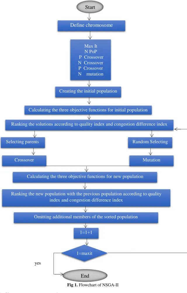
Over the past two decades, genetic algorithms have been considered for its high potential as a new approach to multi-objective optimization problems. The inherent characteristics of genetic algorithms represent the reasons for the suitability of genetic search for multi-objective optimization problems. The main features of the genetic algorithm are multi-directional and global search for maintaining a population of good solutions from generation to generation. The generation-to-generation approach is helpful when reviewing Pareto solutions. The flowchart of this algorithm is as follows:

(11)

154 yes

Fig 1. Flowchart of NSGA-II

5-2-1- Chromosome representation

An appropriate chromosome design is one of the most important steps to achieve a suitable algorithm. Then extraction of the solution of the problem from this chromosome is important. IN the

Start

Define

chromosome

Max It N PoP P Crossover N Crossover P Crossover N mutation

Creating the initial population

Calculating the three objective functions for initial population

Ranking the solutions according to quality index and congestion difference index

Selecting parents Random Selecting

Crossover Mutation

Calculating the three objective functions for new population

Ranking the new population with the previous population according to quality index and congestion difference index

Omitting additional members of the sorted population

1=1+1

1=maxit

(12)

155

algorithm in order to represent the solution, a bi-part chromosome is used that the first part is the selection of the distribution warehouse, and the second part determines the routing of the vehicles. The first part of the chromosome consists of a string with the length of the number of candidate points for the construction of the warehouse. Each of the arrays of this string corresponds to a candidate point and its value is defined as real numbers in the interval [0, 1].

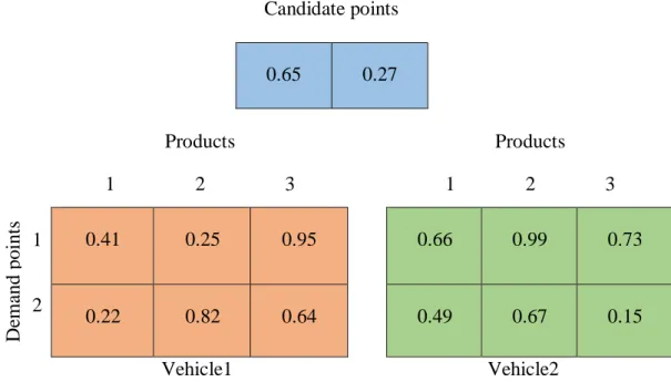
To determine the point to build a warehouse by using this part of the chromosome, we select the point where the corresponding value corresponds to the highest value among the values for the other candidate points as the point of view for the construction of the warehouse. The second part of the chromosome is responsible for routing vehicles. Here we have a three-dimensional matrix with dimensions (number of means of transport × number of product type’s × number of customers). The elements of the matrices are formed as in the previous section of the actual values in the range [0 1], which indicates the priority of allocating vehicles to customers’ demands. Suppose that in a sample we have two candidate points for warehouse construction, three customers, two types of products that the customers’ demands are known. These demands must be delivered to customers by using two vehicles. Figure 2-3 depicts a sample chromosome for the considered problem.

Candidate points

0.65

0.27 Products

1 2 3

Products

1 2 3

0.73

0.99

0.66

0.95

0.25

0.41

1

2 De

mand

point

s

0.15

0.67

0.49

0.64

0.82

0.22 Vehicle1 Vehicle2

Fig 2. Sample chromosome for the considered problem

According to the chromosome presented in figure 2, the chromosome in location 1 has the highest priority. Thus, it is selected as the location of the warehouse. After this step, it is necessary to route the vehicles to service to the demand points according to the second part of the chromosome.

For this purpose, in the second part of the chromosome, the highest priority is the customer's second product at point one that must be shipped with the second vehicle. If this vehicle does not have the ability to carry or contain this product, the next priority will be checked; otherwise, after assigning the intended product of the customer to the second vehicle, the capacity of the vehicle is updated. The routing process continues until all products for all customers are covered.

(13)

156

Table 3. Pareto solutions to ε-constraint method

Round Obj_1 Obj_2 Efficiency Time(Minute: Second)

I 3498 17 Efficient 00:00

II 3506 6 Efficient 00:01

1 3498a ₁₇ _Efficient _00:01

2 3504 16 - 00:00

3 3504 15 - 00:01

4 3504a ₁₄ _Efficient _⋮

5 3506 13 - 00:01

⋮ 3506 ⋮ -

12 3506a ₆ _Efficient

13 Infeasible Infeasible

Total run time 00:06

a

Global optimum

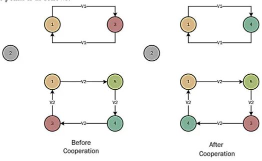
Pareto points amount for two objective functions for 13 cases are shown in Table 3. Since in most cases the solution is acceptable, the results of the method can be trusted. The direction of movement in one of the points is as follows:

Fig 3. The edge Pareto obtained by ε-constraint method before and after cooperation

5-2-2- Adjustment of the parameters of proposed meta- heuristic algorithms

In this section, in order to increase the efficiency of proposed metaheuristic algorithms, we set some levels of the input parameters of the algorithms. Levels of cooperative and non-cooperative factors for big and small problems are shown in tables 4 and 5 respectively.

Table 4. The factors of NSGA-II algorithm along with their levels

Levels in big problems Levels in small problems

factors

Level 3 Level 2

Level 1 Level 3

Level 2 Level 1

150*200 100*300

50*600 100*150

75*200 50*300

Pop*it

0.95 0.9

0.8 0.9

0.85 0.75

Pc

0.2 0.15

0.1 0.15

0.1 0.05

Pm

0.1 0.09

0.07 0.1

0.08 0.06

(14)

157

The design of full factor testing of the four factors mentioned in the NSGA-II algorithm in the case of five types of sample problems and requires 5 × 3 × 3 ^ 4 = 1215 testing for each algorithm if each test is executed 3 times. Therefore, we use the design of fractional experiments. First, we must calculate the degree of freedom.

In this study, we will have one degree of freedom for the total mean and two degrees of freedom for three-level factors. Therefore, the total degree of freedom that is required for the NSGA-II algorithm will be equal to (9 = 1 + 2 × 4).

Tables 5 and 6 show the results non-cooperative and cooperative modes based on SM and MID indicators:

 The MID indicator presents a measurement of the closeness of Pareto's solutions to the ideal point (f1-Best, f2-Best). The lower the distance, the better quality of the solutions.

 The SM indicator determines the uniformity of the width of the set of unanswered responses, and the lower SM, the better quality of the solutions.

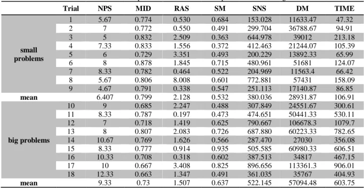
Table 5. Results of the implementation of the non-cooperative NSGA-II algorithm

Trial NPS MID RAS SM SNS DM TIME

small problems

1 5.67 0.774 0.530 0.684 153.028 11633.47 47.32 2 7 0.772 0.550 0.491 299.704 36788.67 94.91 3 5 0.832 2.509 0.363 644.978 39012 213.18 4 7.33 0.833 1.556 0.372 412.463 21244.07 105.39 5 6 0.729 3.351 0.493 200.229 13892.33 65.99 6 8 0.878 1.845 0.715 480.961 51681 124.07 7 8.33 0.782 0.464 0.522 204.969 11563.4 66.42 8 5.67 0.806 8.008 0.601 772.881 57431 158.09 9 4.67 0.791 0.338 0.547 251.113 17140.87 86.85 mean 6.407 0.799 2.128 0.532 380.036 28931.87 106.91

big problems

10 9 0.685 2.247 0.488 307.849 24551.67 300.61 11 8.33 0.787 0.197 0.473 474.651 50441.33 530.11 12 7 0.718 1.419 0.625 790.667 106678.3 1079.7 13 8 0.807 2.083 0.726 687.880 60223.33 782.65 14 10.67 0.769 1.626 0.566 287.470 27030 356.08 15 8.33 0.777 0.914 0.935 505.585 60980.33 606.51 16 10.33 0.708 0.318 0.602 387.513 34817 467.15 17 10 0.667 3.408 0.825 896.656 113361.3 906.01 18 12.33 0.663 1.347 0.491 361.035 35767 404.93 mean 9.33 0.73 1.507 0.637 522.145 57094.48 603.75

Table 6 shows the collaborative mode results based on the SM and mid indicators. As it can be seen, the results of both indicators are between zero and one

.

(15)

158

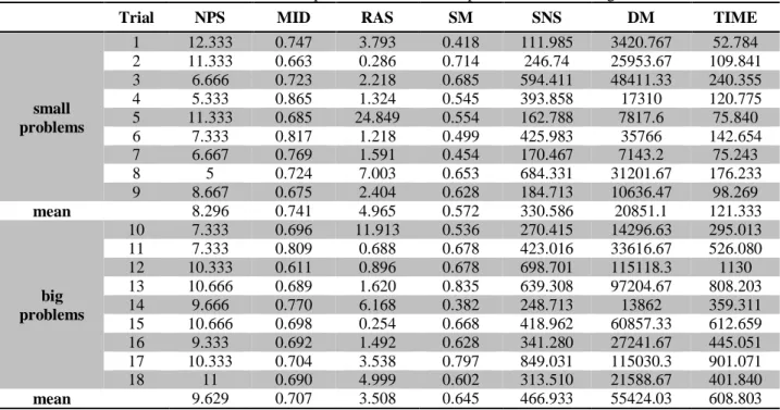
Table 6. Results of the implementation of the cooperative NSGA-11 algorithm

Trial NPS MID RAS SM SNS DM TIME

small problems

1 12.333 0.747 3.793 0.418 111.985 3420.767 52.784 2 11.333 0.663 0.286 0.714 246.74 25953.67 109.841 3 6.666 0.723 2.218 0.685 594.411 48411.33 240.355 4 5.333 0.865 1.324 0.545 393.858 17310 120.775 5 11.333 0.685 24.849 0.554 162.788 7817.6 75.840 6 7.333 0.817 1.218 0.499 425.983 35766 142.654 7 6.667 0.769 1.591 0.454 170.467 7143.2 75.243 8 5 0.724 7.003 0.653 684.331 31201.67 176.233 9 8.667 0.675 2.404 0.628 184.713 10636.47 98.269 mean 8.296 0.741 4.965 0.572 330.586 20851.1 121.333

big problems

10 7.333 0.696 11.913 0.536 270.415 14296.63 295.013 11 7.333 0.809 0.688 0.678 423.016 33616.67 526.080 12 10.333 0.611 0.896 0.678 698.701 115118.3 1130 13 10.666 0.689 1.620 0.835 639.308 97204.67 808.203 14 9.666 0.770 6.168 0.382 248.713 13862 359.311 15 10.666 0.698 0.254 0.668 418.962 60857.33 612.659 16 9.333 0.692 1.492 0.628 341.280 27241.67 445.051 17 10.333 0.704 3.538 0.797 849.031 115030.3 901.071 18 11 0.690 4.999 0.602 313.510 21588.67 401.840 mean 9.629 0.707 3.508 0.645 466.933 55424.03 608.803

As it can be seen, the obtained values are less in the cooperative mode based on the mentioned criteria. This shows that the solutions have high quality and they are close to the Pareto's solutions as well as the better performance of this algorithm.

Fig 4. Comparison of algorithms in terms of the MID evaluation index and the number of products

Fig 5. Comparison of algorithms in terms of the MID evaluation index and the number of potential warehouses

0.65 0.7 0.75 0.8

2 3 5

M

ID

Number of products

0.6 0.65 0.7 0.75 0.8 0.85

3 4 5 6 8 10

M

ID

(16)

159

Figures 4 and 5 also represent a better performance of the cooperative mode in all available problems in terms of the number of products and the number of potential middle warehouses based on the MID index. As it can be seen, blue lines, which are showing the cooperative method, are always above the red lines, which are showing the non-cooperative method. This indicates that the cooperative mode is better on both levels and it has better results in comparison with non-cooperative mode except when the numbers of middle depots are 10 points.

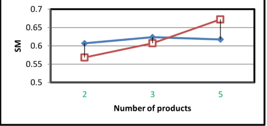
Fig 6. Comparison of algorithms in terms of SM evaluation index and number of products

Fig 7. Comparison of algorithms in terms of SM evaluation index and number of potential warehouses

Figures 6 and 7 also represent the almost identical performance of both cooperative and non-cooperative modes in all available issues in terms of the number of products and the number of potential middle warehouses based on SM. In fact, the spacing criterion calculates the standard deviation of the different values of

d

_i when the answers are uniformly aligned and then the amount of spacing

SM

will be small. Therefore, the algorithm whose non-recursive responses have a small amount of spacing will be more favorable. This indicates that the cooperative mode and non-cooperative mode have the same level of performance at both levels and they do not differ significantly.

6- The Numerical example and its results

In this section, to better understand the model we present a case study of the problem and calculate the fair distribution of cost savings among players.

Given the advancement of urban life and the change in the interests and attitudes of societies, it is inevitable to pay attention to the transfers of people and goods. The ever-increasing advances in industry and mass production have made it extremely important to focus on target markets and how to sell them to attract more market share for manufacturers. Collaborative techniques to allocate cost savings include:

0.5 0.55 0.6 0.65 0.7

2 3 5

SM

Number of products

0.4 0.5 0.6 0.7 0.8

3 4 5 6 8 10

SM

(17)

160

6-1- Shapley Value

This method allocates a certain amount of profit to each player relative to the economic impact of the player in different coalitions. The mathematical expression of the Shapley value is as follows:

(37) xi= ∑

(|s|-1)! (|N|-|S|)! |N|!

i∈S

[v(S)-v(S\ {i}]

6-2- Core method

Another benchmark used to optimize cost savings is core. The game is called stable if the core value is non-empty.

𝑐𝑜𝑟𝑒(0) = {𝑦⃗ ∈ 𝑌|𝑒(𝑠, 𝑦⃗) ≤ 0, ∀⊂ 𝑃} = {𝑦⃗ ∈ 𝑌|𝑣(𝑆) − ∑𝑝∈𝑃𝑦𝑝 ≤ 0, ∀𝑆 ⊂ 𝑃} ( 38 )

6.3. 𝝉

Value:

The next development of Shapley Value is based on the idea of a prior alliance. The 𝜏 value is defined as the effective ratio (ie (𝜏⃗𝜖𝑌), because 𝜏⃗ = 𝑚 + 𝑥(𝑀 − 𝑚) for some 𝛼, in that M and m represent the imaginary efficiency and the minimum wage vector, respectively and they are defined as follows:

𝑚𝑝=𝑚𝑎𝑥_{𝑆𝑚:𝑃́𝜖𝑆𝑚}{𝐶𝑆(𝑆𝑚) − ∑ 𝑀𝑝́ 𝑃́𝜖𝑆𝑚 {𝑃}

} 𝑀𝑝 = 𝐶𝑆(𝑃) − 𝐶𝑆 \ {𝑝})

( 39 )

( 40 )

The 𝜏 value method defines the ratios 𝜏⃗ = (𝜏1, 𝜏2, … , 𝜏𝑛) because 𝜏𝑘 = 𝑚𝑘+ 𝛼(𝑀𝑘+ 𝑚𝑘) Where

𝛼𝜖[0,1] is defined uniquely by ∑ 𝑝 ∈ 𝑃𝜏𝑝 = 𝐶𝑆(𝑃)

6-4- Equal cost saving method (ECSM)

An equal cost-saving method is an incentive to provide a stable and uniform allocation for players. In fact, this method minimizes the maximum difference in cost savings in a two-to-two-way cost between the owners in a coalition. An equal cost-saving method can be formulated as follows:

𝑀𝑖𝑛 𝓏 ( 41 )

𝑆𝑢𝑏𝑗𝑒𝑐𝑡 𝑡𝑜:

𝓏 ≥ |𝑦𝑝− 𝑦𝑝́|, ∀(𝑝, 𝑝′) ∈ 𝑝, ( 42 )

∑ 𝑦𝑝 𝑝∈𝑆

≥ 𝐶𝑆(𝑆), 𝑓𝑜𝑟𝑎𝑙𝑙 𝑆 ⊂ 𝑃, 𝑆 ≠ 𝑃, ( 43 )

∑ 𝑦𝑝 𝑝∈𝑆

= 𝐶𝑆(𝑃) ( 44 )

Constraint set (42) measures the maximum difference between the relatives of each two players. Thus, variable z represents the largest difference that should be minimized in the objective function. Constraint sets (43) and (44) ensure the stability of the imputation. Table 7 shows the output from the numerical example in real-world which is executed by the collaborative algorithm.

(18)

161

Table 7. The result of problem-solving in the collaborative algorithm

Case NPS MID RAS SM SNS DM TIME

collaborative 2 1 9.44E+03 0 720.7986 21.2745 6.53E+03

Table 8. Outputs of the results of collaborative techniques for assigning savings in collaborative mode

Asymmetric information Symmetric information coalition ESCM 𝜏 value Max Core shapely ESCM 𝜏 value Max Core shapely 0.923 0.967 0.96 0.96 4.9 5.054 5.01 4.36

𝑠1= {1}

1.109 0.915 0.9 0.97 4.961 5.072 5.09 5.26

𝑠1= {2}

1.01 1.07 1.00 1.01 4.9701 5.04 5.026 5.37

𝑠1= {3}

0.971 0.912 0.94 1.07 5.102 5.015 5.16 5.67

𝑠1= {4}

1.12 1.078 1.1 1.02 5.201 5.04 5.31 6.01

𝑠1= {5}

7- Managerial insights

The following management insights can be concluded from this study:

1) By using this model and approach, we can minimize and balance the total costs, including fixed costs, and the cost of vehicles movement, the cost of building the warehouse and the total delay of the delivery date.

2) Considering the good performance of the collaborative algorithm, the cost savings are significant and this factor can be considered as an incentive for cooperation between companies.

3) The results of the cooperative game theory techniques are different, and the cost savings of each player can be specified by considering these features in the contract between companies. Given the fact that the model is arranged for location-routing-arc in a collaborative approach, doing these things properly can have dramatic effects on chain efficiency and these actions are of particular importance due to their nature.

The nature of the corruption and unpredictability of the time of food corruption requires comprehensive plans to reduce and mitigate the risks and consequences of their deterioration. Planning to deal with such outcomes and public awareness has reduced death and the loss of assets and illnesses, which is, in fact, the main focus of responses and therapeutic reactions.

One of the possible strategies for the cost of transporting corrupt materials is to locate and store inventory near the desired site. (American Health Organization, 2011).

Therefore, in order to achieve the objectives of supply chain management of corrupt materials, routing is a potential field that can greatly improve and location inventory warehouse special logistic strategies to respond faster and better.

Since in these situations, usually there is a shortage of resources, goods, and vehicles for optimum customer satisfaction, proper planning to achieve the goal of efficiency and effectiveness of accountability with regard to resources and facilities is of paramount importance that managers should pay special attention to them. Therefore, the correct use of the results of this research will lead to strategic planning in the organizations and can r improve the supply chain of corruptible goods.

8- Conclusion and future research

In this study, the problem of location-routing-arcs is studied by using game theory.

Here, the goal is to select a location from potential locations as a warehouse and to determine the route and delivery of vehicles for delivery and receipt of customer requests in such a way that, firstly, restrictions such as the capacity of the vehicles and their ability should be considered, and Secondly, there is a goal of balancing between minimizing the total costs ( including fixed costs and the movement of vehicles, the cost of building the warehouse) and minimizing the total amount of delays from the timing of the delivery. In order to solve the problem, an integer linear mathematical model is presented that can solve the problem in small dimensions. But due to Np-hardness of the problem in big dimensions, NSGAII meta-heuristic approach is used in cooperative and non-cooperative modes.

(19)

162

Statistical surveys show that MID index in the cooperative method is significantly better in comparison with the NSGA-II algorithm and SM index in both algorithms is at the same level and does not make any significant difference. Thus, there are some possible directions for future research. Considering supply and demand data in fuzzy or fuzzy type 2 can be one of the research ideas for future studies. In this research, the delivery time is scheduled to take place at a specified time, and the delivery of the product after this time will result in paying fines. But, it is possible that some customers tend to receive products at certain times of the day for various reasons.

Therefore, considering a customer window to receive products and delivering the products out of that window leads to paying fines. Moreover, considering random uncertainty in the problem and solving the model by stochastic planning and modified PSO can be of great importance.

References

Ahmadi, T., Karimi, H., Davoudpour, H., & Hosseinijou, S. A. (2015). A robust decision-making approach for p-hub median location problems based on two-stage stochastic programming and mean-variance theory: a real case study. The International Journal of Advanced Manufacturing

Technology, 77(9-12), 1943-1953.

Javid, A. A., & Azad, N. (2010). Incorporating location, routing and inventory decisions in supply chain network design. Transportation Research Part E: Logistics and Transportation Review, 46(5), 582-597.

Cooper, L. (1963). Location-allocation problems. Operations research, 11(3), 331-343.

Doulabi, S. H. H., & Seifi, A. (2013). Lower and upper bounds for location-arc routing problems with vehicle capacity constraints. European Journal of Operational Research, 224(1), 189-208.

Ghorbani, A., & Jokar, M. R. A. (2016). A hybrid imperialist competitive-simulated annealing algorithm for a multisource multi-product location-routing-inventory problem. Computers & Industrial Engineering, 101, 116-127.

Dantzig, G. B., & Ramser, J. H. (1959). The truck dispatching problem. Management science, 6(1),

80-91.

Fardi, K., Jafarzadeh_Ghoushchi, S., & Hafezalkotob, A. (2019). An extended robust approach for a

cooperative inventory routing problem. Expert Systems with Applications, 116, 310-327.

Fernández, E., Fontana, D., & Speranza, M. G. (2016). On the collaboration uncapacitated arc routing problem. Computers & Operations Research, 67, 120-131.

Golden, B. L., & Wong, R. T. (1981). Capacitated arc routing problems. Networks, 11(3), 305-315. Hafezalkotob, A., & Makui, A. (2015). Cooperative maximum-flow problem under uncertainty in logistic networks. Applied Mathematics and Computation, 250, 593-604.

Lopes, R. B., Plastria, F., Ferreira, C., & Santos, B. S. (2014). Location-arc routing problem: Heuristic approaches and test instances. Computers & Operations Research, 43, 309-317.

Lozano, S., Moreno, P., Adenso-Díaz, B., & Algaba, E. (2013). Cooperative game theory approach to allocating benefits of horizontal cooperation. European Journal of Operational Research, 229(2), 444-452.

Ma, Z., & Dai, Y. (2010). Stochastic dynamic location-routing-inventory problem in two-echelon multi-product distribution systems. In ICLEM 2010: Logistics For Sustained Economic Development: Infrastructure, Information, Integration (pp. 2559-2565).

Nagy, G., & Salhi, S. (2007). Location-routing: Issues, models and methods. European journal of operational research, 177(2), 649-672.

Razmi, J., Hassani, A., & Hafezalkotob, A. (2018). Cost saving allocation of horizontal cooperation in restructured natural gas distribution network. Kybernetes, 47(6), 1217-1241.

(20)

163

Riquelme-Rodríguez, J. P., Gamache, M., & Langevin, A. (2016). Location arc routing problem with inventory constraints. Computers & Operations Research, 76, 84-94.

Salhi, S., & Rand, G. K. (1989). The effect of ignoring routes when locating depots. European journal of operational research, 39(2), 150-156.

Seyedhosseini, S. M., Bozorgi-Amiri, A., & Daraei, S. (2014). An integrated location-Routing-Inventory problem by considering supply disruption. IBusiness, 6(02), 29.

Shang, R., Du, B., Ma, H., Jiao, L., Xue, Y., & Stolkin, R. (2016). Immune clonal algorithm based on directed evolution for multi-objective capacitated arc routing problem. Applied Soft Computing, 49, 748-758.

Tavakkoli-Moghaddam, R., & Raziei, Z. (2016). A new bi-objective location-routing-inventory problem with fuzzy demands. IFAC-PapersOnLine, 49(12), 1116-1121.

Ting, C. J., & Chen, C. H. (2013). A multiple ant colony optimization algorithm for the capacitated location routing problem. International Journal of Production Economics, 141(1), 34-44.

Tuzun, D., & Burke, L. I. (1999). A two-phase tabu search approach to the location routing problem. European journal of operational research, 116(1), 87-99.

Tütüncü, G. Y., Carreto, C. A., & Baker, B. M. (2009). A visual interactive approach to classical and mixed vehicle routing problems with backhauls. Omega, 37(1), 138-154.

Willemse, E. J., & Joubert, J. W. (2016). Constructive heuristics for the mixed capacity arc routing problem under time restrictions with intermediate facilities. Computers & Operations Research, 68, 30-62.

Xu, Y., & Zhong, H. (2011, January). Benefit mechanism designing: for coordinating three stages supply chain. In Management Science and Industrial Engineering (MSIE), 2011 International Conference on (pp. 966-969). IEEE.

Yao, Z., Lee, L. H., Jaruphongsa, W., Tan, V., & Hui, C. F. (2010). Multi-source facility location– allocation and inventory problem. European Journal of Operational Research, 207(2), 750-762. Yali, H. C. Y. L. W. (2010). Game Analysis On Stakeholders in the Collective Forest Tenure Reform Of Ecological Forest [J]. Forestry Economics, 7, 008.

Zibaei, S., Hafezalkotob, A., & Ghashami, S. S. (2016). Cooperative vehicle routing problem: an opportunity for cost saving. Journal of Industrial Engineering International, 12(3), 271-286.

Zhang, Y., Mei, Y., Tang, K., & Jiang, K. (2017). Memetic algorithm with route decomposing for periodic capacitated arc routing problem. Applied Soft Computing, 52, 1130-1142.

Zhao, Y., Wang, S., Cheng, T. E., Yang, X., & Huang, Z. (2010). Coordination of supply chains by option contracts: A cooperative game theory approach. European Journal of Operational Research, 207(2), 668-675.