Energy Based Clustering Self Organizing Map
Protocol For Wireless Sensor Networks
Kourosh Dadashtabar Ahmadi
Department of computer engineering Malek Ashtar University of Technology
Tehran, Iran [email protected]
Morteza Barari
Department of computer engineering Malek Ashtar University of Technology
Tehran, Iran [email protected]
Neda Enami
Department of computer engineering Malek Ashtar University of Technology
Tehran, Iran [email protected]
Received: July 20 , 2013-Accepted: December 5, 2014
Abstract—Cluster based routing are the most frequently used energy efficient routing protocols in Wireless Sensor Networks which avoid single gateway architecture through dividing of network nodes into several clusters while in each cluster, Cluster Heads work as local Base stations. However, there is several energy efficient cluster-based protocols in the literature, most of them use the topological neighborhood or adjacency as main parameter to form the clusters. This paper present a new centralized adaptive Energy Based Clustering protocol through the application of Self organizing map neural networks (called EBC-S) which can cluster sensor nodes, based on their energy level and coordinates. We apply some maximum energy nodes as weights of SOM map units; so that the nodes with higher energy attract the nearest nodes with lower energy levels. So a cluster may not necessarily contain adjacent nodes. The new algorithm enables us to form energy balanced clusters and equally distribute energy consumption on whole network space. Simulation results show the considerable profit of our proposed protocol over LEACH and LEA2C (another SOM based protocol); by increasing the network lifetime and insuring more network coverage.
Keywords-energy based clustering; self organizing map neural networks ;wireless sensor networks
I. INTRODUCTION
Wireless Sensor Network (WSN) can be defined as a network consists of several sensor nodes in which each sensor node should have at least sensing, processing and wireless communication capabilities. The most important difference of WSNs with other wireless networks may be their computation and energy resource constraints which usually arise from small size of sensor nodes that is a prerequisite to
WSNs main applications. The main and most important reason of WSNs creation was continuous monitoring of environments where are too hard or impossible for human to access or stay. So there is often low possibility to replace or recharge the dead nodes as well. As a result, energy conservation is the main concern in application of WSNs. Energy conservation should be gained by wisely management
of energy sources. Several energy conservation
schemes have been proposed in the literature while
there is a comprehensive survey of energy conservation methods for WSNs and the taxonomy of all into three main approaches (duty-cycling, data reduction, and mobility based approaches [2]. Also these methods can be divided according to the layer of protocol stack with which they are involved such as several MAC protocols that have been proposed in the literature and survey studies on them as in [9,18]. Today, radio communications are the most energy consuming task of WSNs [21, 22]. So many research studies focused on energy efficient routing protocols to address this problem. Routing protocols can be divided based on different considerations like application, network structure or protocol operation but the most commonly used classification usually divide them into three general categories based on the underlying network structure: flat, hierarchical (cluster based) and
location-based routings [1]. In flat networks, all nodes
typically play the same role and sensor nodes collaborate to perform the sensing task as in SPIN [13, 17], Direct Diffusion [15] etc. In location based routing, sensor nodes are addressed by means of their locations. The sensing area is divided into small virtual grids. All nodes in same virtual grid are equivalent for routing and only one node need to be active at a time. The most famous protocols from this category are GAF [33] and GEAR [34]. Hierarchical or Cluster based routing protocols, as potentially the most energy efficient organization, have shown wide application in the past few years [27,29] and numerous energy efficient clustering algorithms, have been proposed such as LEACH [11,12], PEGASIS [19,22], EECS
[31], HEED[32], EEUC [5], LEACH-C [11] and
LEA2C [7] etc. Hierarchical routing is mainly two-layer routing where one two-layer is used to select cluster heads and the other for routing [1]. In clustering protocols, geographically close nodes are organized into groups and each group is referred to as a cluster. Higher-energy nodes called Cluster Heads (CHs) play the coordination and communication tasks and other nodes in the clusters called normal (simple) nodes only do the sensing job and transmit their data packets to CHs. Because the data from adjacent sensor nodes usually have high correlation, CHs should also aggregate and/or fuse these received data packets to decrease the number of transmitted messages to Base
Station[28].
In this paper we present a novel Energy Based Clustering protocol through using Self organizing map neural networks (called EBC-S). Our work is closely related to LEACH-Centralized [11] according to the Base Station cluster formation method it uses which requires global knowledge about all nodes energy and positions. EBC-S is also related to LEA2C [8] protocol which is another SOM-based clustering protocol. LEA2C handled the NP-hard problem of optimal number of clusters by a two-phase method; SOM followed by Kmeans and it shows a considerable profit compared with another LEACH like protocol, called EECS [31]. The difference of our proposed protocol with previous one is that it is able to adaptively cluster the nodes not only based on their topological closeness (coordinates) but also based on their energy levels in
each set-up phase. So clusters may not necessarily contain adjacent nodes. As the result of forming clusters with near equal energy level, we better can balance the energy consumption in whole network during the data transmission phase and extend the lifetime of the network in the terms of first dead time and insures more network coverage during network life time. Simulation results show the profit of our protocol over LEACH and LEA2C.
II. LEACHPROTOCOL
Low Energy Adaptive Clustering Hierarchy (LEACH) by Heinzelman et al., (2000) is the most famous clustering protocol which had been a basis for many further clustering protocols. The most important goal of LEACH is to have local Base Station (Cluster Heads) to reduce the energy cost of transmitting data from normal nodes to a distant Base Station. In LEACH, nodes organize themselves into local clusters with one node acting as cluster head. All non-cluster head nodes (normal nodes) transmit their data to the cluster heads. Cluster head nodes do some data aggregation and/or data fusion function on which should be transmitted to Base Station. Cluster head nodes are much more energy intensive than normal nodes. So choosing fix cluster heads, will end up in their early death. One solution can be random rotation of cluster head among nodes to balance the energy level of the network. The operation of LEACH is divided into rounds. Each round begins with a set-up (clustering) phase when clusters are organized, followed by a steady- state (transmission) phase when data packets are transferred from normal nodes to cluster heads. After data aggregation, cluster heads will transmit the messages to the Base Station. The election of cluster head is done with a probability function: each node selects a random number between 0 and 1 and if
the number is less than T(n), the node is elected as a
cluster head for current round:
otherwise G n if P r P
P n
T
0
1 mod 1
)
( (1)
Where, P is the cluster head probability, r is the
number of current round and G is the set of nodes that
have not been cluster-heads in last 1/P round. The
strength of LEACH is in its CH rotation mechanism and data aggregation. But one important problem with LEACH is that it offers no guarantee about placement and/or number of cluster head nodes in every round. Therefore using a centralized clustering algorithm would produce better results. LEACH-Centralized (LEACH-C) is a Base Station cluster formation algorithm. It uses the same steady state protocol as LEACH. During the steady state phase, each node sends information about its current position and energy level to BS. The assumption usually is that each node has a GPS receiver. The BS has to insure the evenly distribution of energy among nodes. So it determines a threshold for energy level and selects the nodes (with higher energy than this threshold) as possible cluster heads. The problem of determining the optimal number
of cluster heads is an NP-Hard problem. LEACH-C
makes use of Simulated Annealing (Murata and
Ishibuchi, 1994) algorithm to address this problem. After determining the cluster heads of current round, BS sends a message containing cluster head ID for each node. If a node's cluster head ID matches its own ID, the node is a cluster head; otherwise it's a normal node and can go to sleep until data transmission phase. LEACH-C is more efficient than LEACH (LEACH-C delivers about 40% more data per unit energy than LEACH) because the BS has global knowledge of the location and energy level of all nodes in the network [12]. Also LEACH-C, unlike LEACH, always can
insure the existence of K optimal number of cluster
heads in every set-up phase [11,12].
III. SOMBASED ROUTING PROTOCOLS
Today, Neural Networks can be applied as effective tools in all aspects of reducing energy consumption such as duty cycling, data driven and mobility based approaches in WSNs [10]. Dimensionality reduction, obtained simply from the outputs of the neural-networks clustering algorithms, leads to lower communication costs and energy savings [16].
The Self-Organizing Map (SOM) is an
unsupervised neural network structure consists of neurons organized on a regular low dimensional grid [25]. Each neuron is presented by an n- dimensional
weight vector where n is equal to the dimensions of
input vectors. Weight vectors (or synapses) connect the
input layer to output layer which is called map or
competitive layer. The neurons connect to each other with a neighborhood relation as shown in figure 1. Every input vector activates a neuron in output layer (called winner neuron) based on its most similarity. The similarity is usually measured by Euclidian distance of two vectors.
2 1 ,
ni i j i
j
W
x
D
(2)Where xiis the ith input vector,Wi,j is the weight
vector connecting input i to output neuron j and Djis
the sum of Euclidian distance between input sample xi
and it's connecting weight vector to jth output neuron
which is called a map unit.
Figure 1. SOM topology structure [33]
The important difference of a SOM training algorithm with other vector quantization algorithms is that not only the best matching units (the winner neuron) but also its topological neighbors would be updated. Close observations in input space would
activate two close units of the SOM. The learning phase continues until the stabilization of weight vectors.
)
(
. , ,, ,
old j i i j i old
j i new
j
i
W
h
x
W
W
(3)Where x.iis the input sample, Wi,jold is the previous
weight vector between input vector xiand weight
vector connected to output neuron j , hi,j is the
neighborhood function and Wi,j new is the updated
weight vector between input neuron i and output
neuron j.
There are different applications for SOM neural networks in WSNs energy efficient routing protocols. These applications can be divided into three general groups: path discovery, selection of cluster heads and clustering of nodes. The authors in [3] used Kohonen SOM neural networks for clustering and their analysis to study unpredictable behaviors of network parameters and applications. Clustering of sensor nodes using Kohonen Self Organizing Map (KSOM) is computed for various numbers of nodes by taking different parameters of sensor node such as direction, position, number of hops, energy levels, sensitivity, latency, etc. Authors in [23] proposed a new method for routing in WSNs in which each wireless node use a SOM neural network to decide about containing the data packet and participate in routing or dropping the packet. The assumption of their algorithm is that every node has an importance due to its role in routing so that the nodes which are used more than other nodes in routing due to their positions have more importance. They defined a Network Life Time (NLT) parameter which is sum of the nodes importance in routing at time t and the amount of energy consumption of node for routing As soon as a packet arrives, its feature vector will be extracted and this vector will be sent to SOM of that node. The goal is to maximize NLT parameter. If the node wins the competition against other nodes, it is allowed to send the packet and participate in routing. Otherwise it should drop the packet. SIR [4] is another QoS-driven SOM based routing protocol in which a SOM neural network is introduced in every node to manage the routes that data have to follow. Also [6] proposed a new LEACH like routing protocol in which the election of Cluster Heads is done with SOM neural networks where SOM inputs are intended parameters for cluster heads. SOM cluster the nodes according to their cluster head qualities. However a minimum separation filter should be applied on SOM output then to ensure a minimum separation distance between selected CHs. Results show a 57 % profit of this protocol over LEACH (in terms of first dead time). Low Energy Adaptive Connectionist Clustering (LEA2C) by [7] is another LEACH-C [11,12] like SOM-Based clustering protocol. The cluster formation is done by Base Station in the similar way said for LEACH-C. LEA2C uses a two phase clustering method, SOM followed by Kmeans. The inputs to SOM are the coordinates of sensor nodes in network space. LEA2C apply the connectionist learning by the minimization of the distance between the input
samples (sensor nodes coordinates) and the map prototypes (referents) weighted by an especial neighborhood function. After set-up phase, the cluster heads of every cluster are selected according to one of the three criterions, max energy node, nearest node to BS and nearest node to gravity center of each cluster. Then the transmission phase starts and normal nodes send their packets to their CHs and on to the BS. In the case of using max energy factor for cluster head selection, the protocol would have a cluster head rotation process after every transmission phase. The transmission phase continues until the occurrence of first dead in the network. After that, the re-clustering (set-up) phase will repeat. The simulation results show the profit of LEA2C over another LEACH-based protocol, called EECS [30] (In terms of 50 percent longer lifetime and insuring the network coverage during 90 percent of its total lifetime).
IV. PROPOSED ALGORITHM
In order to use the effectiveness of cluster-based routing algorithms in increasing of WSNs lifetime, we tried to present a new Energy Based Clustering Self organizing map (EBC-S). The motivation of creating EBC-S was inattention of previous clustering algorithms to energy level of the nodes as a key parameter to cluster formation of the networks. We tried to develop the classic idea for topological clustering and incorporate a topologic-energy based clustering method in order to approach to our main goal in WSNs, extending life time of the network. In our idea, energy based clustering can create clusters with equivalent energy levels. In this way the energy consumption would be balanced better in whole network.
A. Algorithm Assumptions
The proposed algorithm is more like LEACH-C and LEA2C protocols. Thus the assumption about BS cluster formation tasks and energy consumptions models of normal and cluster head nodes are the same as previous. The operation of the algorithm is divided into rounds in a similar way to LEACH-C. Each round begins with a cluster setup phase, in which cluster organization takes place, followed by a data transmission phase, throughout which data from the simple nodes is transferred to the cluster heads. Each cluster head aggregates/fuses the data received from other nodes within its cluster and relays the packet to the base station. In every cluster setup phase, Base Station has to cluster the nodes and assign appropriate roles to them. After determining the cluster heads of current round, BS sends a message containing cluster head ID for each node. If a node's cluster head ID matches its own ID, the node is a cluster head otherwise it is a normal node. BS also creates a Time Division Multiple Access (TDMA) table for each cluster and affects this table to CHs. Using TDMA, schedules the data transmission of sensor nodes and also allows sensor nodes to turn off their antennas after their time slot and save their energy. So the energy cost for cluster formation is just for BS and there are no control packets for sensor nodes. We assume that BS has no constraint about its energy resources. Also we assume that BS has
total knowledge about the energy level and position of all nodes of the network (most probably by using GPS receiver in each node). The other important assumption of the protocol is random distribution of nodes in network space. The sensor nodes are homogenous, means they have the same processing and communication capabilities and the same amount of energy resources (at the beginning).
B. Cluster Setup phase
The protocol uses a two phase clustering method SOM followed by Kmeans algorithm which had been proposed in [25] with an exact comparison between the results of direct clustering of data and clustering of the prototype vectors of the SOM. We selected SOM for clustering because it is able to reduce dimensions of multi-dimensional input data and visualize the clusters into a map. In our application, dimensions of input data relates to the number of variables (parameters) that we need to consider for clustering. The reason for using SOM as preliminary phase is to make use of data
pretreatment (dimension reduction, regrouping,
visualization...) gained by SOM [7]. Therefore the data set is first clustered using the SOM, and then, the SOM is clustered by kmeans.
The variables that we want to consider as SOM input dataset is X and Y coordination of every node in network space and the energy level of them. So we will
have a D matrix with n3 dimensions. Since we are
applying two different type variables, first we have to normalize all values. We used a Min-Max
normalization method [26] in which minaandmaxaare
the minimum and maximum values for attribute a.
Min-max normalization, maps a value v in the range of (0, 1) by simply computing:
) min (max min a a a v V (4)
So by means of above equation, our dataset matrix would be: max max 1 max max 1 max 1 max 1 . . . . . . . . . E E yd yd xd xd E E yd yd xd xd D n n (5)
Where D is the data sample matrix or input vectors
of SOM, XD=(xd1...xdn) are X coordinates,
Y=(yd1…ydn)are Y coordinates, E=(E1…En) are energy
levels (remained energy) of all sensor nodes of the
networks, xdmaxis the maximum value for x coordinate
of the network space, ydmax is the maximum value for
Y coordinate of network space and Emax is the remain
energy of maximum energy node of the network( at the
beginning it is equal to Einitial).
In order to determine weight matrix, Base Station
has to select m nodes with highest energy in the
network. At the beginning, the nodes have equal energy level according to our assumptions. So we can
partition the network space to m regions and select the nearest node to center of every region. However due to using two phase SOM-Kmeans method, we usually need to consider a rather large value for m, especially in large WSNs. In this case we can choose the m nodes randomly. We need three variables of these selected (high energy) nodes to apply them as weight vectors of
our SOM: their x coordinate, their y coordinate and
their energy level. Therefore our weight matrix would be: max max 1 max max 1 max max 1 1 . . . 1 . . . . . . E E E E yd yd yd yd xd xd xd xd W m m m (6)
Where W is the weight matrix of SOM, XD=
(xd1...xdn) are x coordinates, YD= (yd1…ydn) are y
coordinates and (1-E1/Emax…1-En/Emax) are consumed
energy of m selected max energy sensor nodes. As you
can see in equation (6), we have a 3m weight vector,
so we would also have m map units (clusters). We
made a change in third variable (remain energy) of selected nodes. In this way we want to move the nodes with less energy towards max energy nodes in order to form balanced clusters in the terms of energy level. So the SOM topology structure would be as figure.2:
Figure 2. SOM topology structure in EBC-S protocol
In our application, learning is done by minimization of Euclidian distance between input samples and the map prototypes weighted by a neighborhood function
hi,j.So thecriterion to be minimized is defined by [7]:
N k M j k j X N jSOM
h
w
x
N
E
k 1 2 1 ) ( . ) ( , ( )1
(7)Where N is the number of data samples, M is the
number of map units; N(xk) is the neuron having the
closest referent to data sample x(k) and h is the Gaussian
neighborhood function defined by:
Where 2
i j r
r the distance between map unit j
and sample input i and
t is the neighborhood radiusat time t which is defined by:
Where t is the number of iteration, T is the maximum number of iteration or the training length.
The distance between Xk and weight vectors of all map
neurons are computed. A neuron N(Xk) which has the
minimum distance with input sample Xk, would win the
competition phase: 2 . 1
min
arg
)( j k
m j
k W X
X
N
(10) The neighborhood radius is a great value at the beginning and it will reduce with increasing of the time of the algorithm in every iteration. After competition phase, SOM should update the weight vector of the
winner N(Xk) and all its neighbors which placed at the
neighborhood radius of (R N(Xk)). If ( )
. k X N j
R
W
then ElseWhere
h
, ( )(
t
)
k
X N
j is the neighborhood function
at time t and (t) is the linear learning factor at time
t define by:
) 1 ( )
(t 0 tT
(13) Where
0
the initial learning rate, t is the numberof iteration and T is the maximum training length. The learning phase repeats until stabilization (no more
change) of weight vectors. SOM clusters n data
samples into m map units (clusters). Now the SOM
should be given to K-means algorithm as input.
K-means, partitions the data set into K subsets
(clusters) such that all objects in a given dataset are closest to the same centroid. K-means randomly selects K of objects as cluster centroids. Then other objects are assigned to these clusters based on minimum Euclidean distance to their centroids. The mean of every cluster is recomputed as new centroids and the operation will continue until the cluster centers do not change anymore. The criterion to be minimized in K-means is defined by:
2 1 1
Ck xQ
k means K k C x C
E (14)
Where C is the number of clusters, Qkis Kth cluster,
Ck is the centroid of cluster Qk.
The best value for K (optimal number of clusters) can be determined with an index. We selected Davies-Bouldin index. DB index actually compute the ratio of
intra-clusters dispersion to inter-cluster distances by: 2 2 , 2 exp ) ( t i j j i r r t h (8) )) ( . ) ( ( ) ( ) ( ) ( ) 1 ( ) ( , .
. t W t t h t xt W t
W j
x N j j
j
k k (11)
)
(
)
1
(
..
t
W
t
W
j
j (12)
tT
t) exp( 0
(9)
Ck ce k l
l c k c k l DB Q Q d Q S Q S C I
1 ( , )
) ( ) ( max 1 (15) With k i k i k c Q c x Q S
2 )( (16)
2
)
,
(
k l k lcl
Q
Q
c
c
d
(17)Where C is the number of clusters, Sc is the
intra-cluster dispersion and dcl is the distance between
centroids of two clusters k and l.
Small values of DB index correspond to clusters which are compact, and whose centers well separated from each other. Consequently, the number of clusters that minimizes DB index is taken as the optimal number of clusters.
Now, Base station knows the optimal number of clusters and their member nodes. So the next step before going to transmission phase is selection of suitable cluster heads for each cluster and assigning appropriate roles to each node.
C. Cluster Head selection phase
Different parameters can be considered for selecting a CH in a formed cluster. In [7,8] three criterions have been considered for CH selection:
1- The sensor having the maximum energy level 2- The nearest sensor to the BS
3- The nearest sensor to gravity center (centroid) of the cluster.
When we select the nearest node to BS in a cluster as CH, we insure to consume least energy to transmit the messages to BS. Also the nearest sensor to gravity center (centroid) of the cluster insure least average energy consumption for intra cluster communications while the reduction of CH overhead is not guaranteed. The results from LEA2C showed that the selecting the nodes with maximum energy level (first factor) as cluster head, gives the best results. This profit over two other criterions might be cause of having CH rotation. Because in the case of two other criterions (nearest sensor to BS or cluster centroid) the selected CHs stay fixed during the transmission phase until next re-clustering phase which may last for several rounds and it will cause the rapid depletion of that CHs, While applying these two criterions showed a longer lifetime (last dead) results.
After determining the cluster head nodes, BS assign appropriate roles to all nodes through the method mentioned for LEACH-C protocol before.
D. Transmission phase
After formation of clusters and selecting their related cluster heads, now it's time to send data sensed at normal nodes to their related cluster heads and after applying data aggregation functions to received packets by CHs, send messages on to the base station. The energy consumption of all nodes is computed. As
in [8,12] the energy consumed for transmission of k
bits of data over a distance d is computed by:
) , ( ) ( ) ,
(k d E l E k d
ETx Txelec Txmp
(18) else d k d k E k d d if d k d k E k d k E mp elec crossover fs elec Tx 4 2 * * ) , ( * * * ) , ( * ) , ( (19)
The energy consumption for receiving k bits of data from a distance d is computed by:
elec elec
Rx
Rx
k
d
E
k
k
E
E
(
,
)
(
)
.
(20)
Where Eelec is the energy of electronic
transmission/reception, k is the size of message in bit, d is the distance between transmitter and receiver, Etx_mp is amplification energy,
is amplificationfactor, dcrossover is a threshold distance over which
transmission factors change (if the distance d is less
than a threshold dcrossover, the free space (fs) model is
used; otherwise, the multipath (mp) model is used Also energy consumption of data aggregation of CHs is:
msg bit nJ
EDA5 / / (21)
After every transmission phase, we count a new round and would have a cluster head rotation (in the case of using maximum energy criterion) as described in last section. But how often should we have a re-clustering phase? Since our goal is to create clusters with equal energy levels, we should have a threshold for re-clustering phase according to variation of energy level of the nodes. The best time for re-clustering can be when a relative reduction occurs in energy level of nodes. So the energy level of m selected highest energy nodes are checked regularly. These nodes are cluster heads of last setup phase. The condition can be the depletion of a predefined percent of their energy level. This threshold energy level is defined experimentally. In this paper, 20 percent depletion of initial energy for first time re-clustering phase and 5 percent depletion for next times are used. When the re-clustering threshold is satisfied, BS sends a re-clustering message to whole network. So, we can summarize the algorithm into following steps:
1- Initialization: random deployment of N
homogeneous sensors in a given space and with the same energy level.
2- Cluster set-up phase:
2.1- clustering of WSN through SOM and K-mean clustering method by using sensor coordinates and remained energy as SOM inputs and selecting of m nodes with maximum energy level as the weights of SOM units using
Eqs. (5) to (17). The value for m can be
different for every scene and experimental. 2.2- selection of cluster heads for every cluster
with one of the 3 criteria mentioned (maximum energy sensor, nearest sensor to BS and nearest sensor to gravity center of the cluster). 2.3- assigning roles to every node (CH or Normal
node) by BS.
3- Data Transmission Phase
3.1- Data transmission from normal nodes to
CHs. Energy consumption of nodes
transmission and CHs reception then computed using energy model and Eqs (19) and (20) 3.2- Data aggregation and or fusion of received
packets and sending results to BS by CHs. energy consumption of CHs is then computed using Eqs (19) and (21)
3.3- CH selection if the CHs had been chosen according to maximum energy criteria 3.4- Repeat the steps 3-1 to 3-4 until the average
energy level of m selected maximum energy nodes show a 20 percent reduction for first time re-clustering and 5 percent for next times.
4- Repeat the steps 2 to 3 until all sensors in the network die.
V. SIMULATIONS AND RESULTS
MATLAB is used to simulate and compare the proposed algorithm (EBC-S) with previous works. To compare proposed protocol results with previous similar protocol (LEACH and LEA2C) we used the energy models as in Esq. (18) to (21) and scenes according to table1. SOM toolbox proposed by Helsinki University of Technology (HUT) researchers has been used to simulate proposed algorithm [25]. Also the data in table1 were used to present an exact comparison with three protocols (LEACH, LEA2C and EBC-S) results with different number of nodes (two scenes).
The other parameter that should be defined in
simulation is the value for m (number of maximum
energy level nodes that we use as SOM weights). This number is selected experimentally and its value is in relation with optimal number of clusters that we expected to have. In first scene (100 nodes), we assume m=16 or 20 and in second scene (400 nodes) m=50 or 80.
Table1: Parameters of simulation
The EBC-S protocol performance was evaluated with three criterions for cluster head selection used by
[7]. The results show that selection of maximum energy node as CH, always give the best performance far enough from two other criterions (nearest sensor to BS or nearest sensor to GC). So the best performance of EBC-S (with CH maximum energy) has been compared with two other previous protocols; LEACH and LEA2C for two scenes with characteristics mentioned in table1. The comparison was done through using of three metrics: the number of round (time) when first node dies (First dead time), the number of round (time) when half of nodes die (Half dead time) and the number of round (time) when last node dies (Last dead time).the results are shown in table (2 ,3).
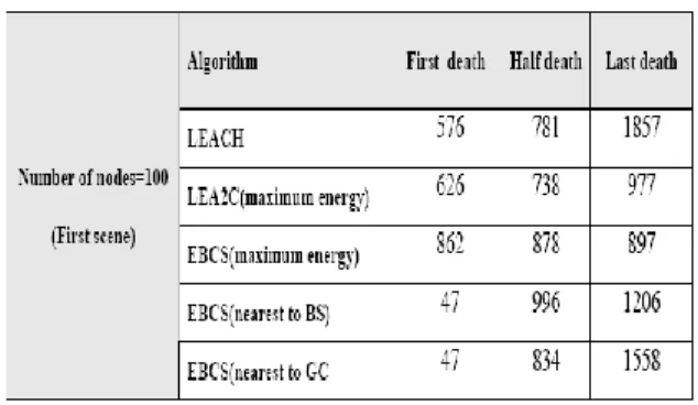
Table 2: comparison of algorithms results (first scene)
Table3. Comparison of algorithms results (second scene)
In figures (3.a, 4.a) you can see the advantages of the proposed protocol compared with others. The results on figures (3.a, 4.a) show that the proposed algorithm can insure total survival (network coverage) during 95% of network lifetime in first scene and 90% in second scene.
As shown in figure (3.a), the new algorithm can increase the lifetime of the network up to 50% over LEACH and 38 % over LEA2C protocols (for the first scene and with maximum energy CH criterion).Also results shown on figure (4a) prove that the new algorithm increase the lifetime of the network up to 27% over LEACH and 11% over LEA2C protocols (for the second scene and with maximum energy CH criterion).
3(a)
3(b)
Figure 3. Number of alive nodes VS time (a) comparing in LEACH, LEA2C and EBC-S (proposed algorithm) (b) comparing in EBCS (proposed algorithm) with different CH criterions (First Scene)
In figures (3.b, 4.b) the performance of using two other CH selection criterions (nearest node to Gravity Center of the cluster and nearest node to Base Station) have been compared to maximum energy criterion. As you can see, the performances of two other criterions are very near to each other while they are too far from
maximum energy criterion performance.
4(a)
4(b)
Figure 4. Number of alive nodes VS time (a) comparing in LEACH, LEA2C and EBC-S (b) comparing in EBCS (proposed algorithm) with different CH criterions (Second
scene)
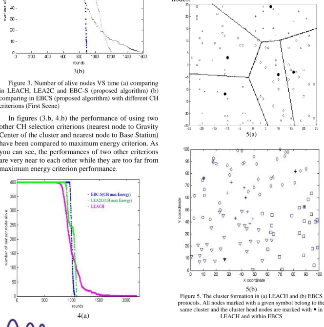
In figure (5) you can see the cluster formation situation and dispersion of cluster nodes in LEACH and EBCS protocols. As it is shown in EBCS unlike LEACH, the boundaries of clusters are unlimited and each cluster does not necessarily contain adjacent nodes.
5(a)
5(b)
Figure 5. The cluster formation in (a) LEACH and (b) EBCS protocols. All nodes marked with a given symbol belong to the
same cluster and the cluster head nodes are marked with in LEACH and within EBCS
VI. CONCLUSIONS
In this paper we proposed a new Energy Based Clustering protocol through SOM neural networks (called EBC-S) which applies energy levels and coordinates of nodes as clustering input parameters and uses some nodes with maximum energy levels as weight vectors of SOM map units. Nodes with maximum energy attract nearest nodes with lower energy in order to create energy balanced clusters. The clustering phase performs by a two phase SOM-Kmeans clustering method. The simulation results show 50% Profit of new algorithm over LEACH and 38% profit over LEA2C (in first scene) and 27% profit over LEACH and 11% profit over LEA2C (in second scene) in the terms of increasing first dead time while ensuring total coverage during 90% up to 95% of network life time in two scenes. The way of cluster formation in EBCS is different from other algorithms and a cluster does not necessarily consist of adjacent nodes. As future works, the following research areas would improve the protocol results:
Combination of proposed algorithm with
multi- hoping routing protocols.
Applying other useful parameters for clustering
Applying different structures for SOM and
Kmeans algorithms
Applying different criterions for Cluster Head
selection of the protocol.
Applying different neighborhood functions to
optimize SOM clustering
REFERENCES
[1] Al-karaki J.N, Kamal A.E. Routing Techniques in Wireless Sensor Networks: A Survey, IEEE Wireless Communication, 2004, p.6-28
[2] Anastasi G, Conti M, Passarella A. Energy Conservation in Wireless Sensor Networks: a survey. In: Ad Hoc Networks, volume 7, Issue 3, Elsevier; 2009, p.537-568
[3] Aslam N, Philips W, Robertson W, Siva Kumar SH. A multi-criterion optimization technique for energy efficient cluster formation in Wireless Sensor networks. In: Information Fusion, Elsevier; 2010
[4] Barbancho J, Leon C, Molina F.J, Barbancho A. Using artificial intelligence in routing scheme for wireless networks. In: Computer Communications 30, Elsevier; 2007, pp. 2802-2811
[5] Chengfa L, Mao Y, Guigai C. An Energy-Efficient Unequal Clustering Mechanism for Wireless Sensor Networks. In: Proc. Of IEEE MASS. 2005
[6] Cordina M, Debono C.J. Increasing Wireless Sensor Network Lifetime through the Application of SOM neural networks. In: ISCCSP, IEEE, Malta, 2008, p. 467-471
[7] Dehni L, Kief F, Bennani Y. Power Control and Clustering in Wireless Sensor Networks. In: Proceedings of Med-Hoc-Net 2005: Mediterranean Ad Hoc Networking Workshop, France. [8] Dehni L, Krief F, Bennani Y. Power Control and Clustering in
Wireless Sensor Networks. In: Challenges in Ad Hoc Networking, vol 2005, p.31-40.
[9] Demirkol I, Ersoy C, Alagoz F, MAC Protocols for Wireless Sensor Networks: a Survey. In: IEEE Communications Magazine, 2006
[10] Enami N, Askari Moghadam R, Haghighat A. A Survey on Application of Neural Networks in Energy Conservation of Wireless Sensor Networks. In: Recent Trends in Wireless and
Mobile Networks, WiMo 2010 Proceedings, Ankara, Turkey, 2010. p. 283–294.
[11] Heinzelman W, Chandrakasan A, Balakrishnan H. Application-specific protocol architecture for wireless microsensor networks. In: IEEE Transactions on Wireless Communications, 2002, p. 660 - 670.
[12] Heinzelman W, Chandrakasan A, Balakrishnan H. Energy-Efficient Communication Protocol for Wireless Microsensor Networks. In: Proc. 33rd Hawaii Int’l. Conf.Sys. Sci, 2000 [13] Heinzelman W, Kulik J, Balakrishnan H. Adaptive Protocols
for Information Dissemination in Wireless Sensor Networks. In: Proc. 5th ACM/IEEE Mobicom, Seattle, WA, 1999, p. 174– 85.
[14] Heinzelman W. Application-Specific Protocol Architectures for Wireless Networks. In: PhD Thesis, Massachusetts Institute of Technology, 2000
[15] Intanagonwiwat C, Govindan R, Estrin D. Directed Diffusion: a Scalable and Robust Communication Paradigm for Sensor Networks. In: Proc. ACM Mobi-Com 2000, Boston, MA, 2000, p. 56–67.
[16] Kulakov A, Davcev D, Trajkovski G. Application of wavelet neural-networks in wireless sensor networks. In: Sixth International Conference on Software Engineering, Artificial Intelligence, 2005, pp. 262–267
[17] Kulik J, Heinzelman W. R, Balakrishnan, H. Negotiation-Based Protocols for Disseminating Information in Wireless Sensor Networks. In: Wireless Networks, vol. 8, 2002, pp. 169–85.
[18] Langendoen K, Medium Access Control in Wireless Sensor Networks. In: Book Chapter in “Medium Access Control in Wireless Networks, Volume II: Practice and Standards”, Nova Science Publishers, 2008.
[19] Lindsey S, Raghavendra C. PEGASIS: Power-Efficient Gathering in Sensor Information Systems. In: IEEE Aerospace Conf. Proc., vol. 3, 9–16, 2002, pp. 1125–30.
[20] Murata T, Ishibuchi H. Performance evaluation of genetic algorithms for flowshop scheduling problems. In: Proc. 1st IEEE Conf. Evolutionary Computation, vol. 2, 2008, pp. 812– 817.
[21] Pottie G, Kaiser W, Wireless Integrated Network Sensors. In: Communication of ACM, Vol. 43, N. 5, pp. 51-58, May 2000. [22] Raghunathan V, Schurghers C, Park S, Srivastava M. Energy-aware Wireless Microsensor Networks. In: IEEE Signal Processing Magazine, March 2002, pp. 40-50.
[23] Shahbazi H, Araghizadeh M.A, Dalvi M. Minimum Power Intelligent Routing In Wireless Sensors Networks Using Self Organizing Neural Networks. In: IEEE International Symposium on Telecommunications, 2008, p. 354–358 [24] Vesanto J, Alhoniemi E. Clustering of Self Organizing Map.
In: IEEE Transactions on Neural Networks, Vol. 11, No. 3, 2000, pp. 586-600.
[25] Vesanto J, Himberg J, Alhoniemi E, Parhankangas J. Self-Organizing Map in MATLAB: The SOM toolbox. In: Proc of MATLAB DSP Conference, Finland, 1999, p.35-40 [26] Visalakshi N. K, Thangavel K. Impact of Normalization in
Distributed K-Means Clustering. In: International Journal of Soft Computing 4, Medwell journal, 2009, p. 168-172. [27] Vlajic N, Xia D. Wireless Sensor Networks: To Cluster or Not
to Cluster? In: Proc. of WoWMoM, 2006
[28] Wei D, Kaplan SH, Chan H.A. Energy Efficient Clustering Algorithms for Wireless Sensor Networks. In: IEEE Communication Society workshop proceeding, 2008. [29] Wei D. Clustering Algorithms for Sensor Networks and
Mobile Ad Hoc Networks to Improve Energy Efficiency, PhD thesis, 2007, University of Cape Town.
[30] Xu Y, Heidemann J, Estrin D. Geography informed Energy Conservation for Ad-hoc Routing. In: Proc. 7th Annual ACM/IEEE Int’l. Conf. Mobile Comp and Net, 2001, pp. 70– 84.
[31] Ye M, Li C. F, Chen G. H, Wu J. EECS: An Energy Efficient Clustering Scheme in Wireless Sensor Networks. In: Proceedings of IEEE Int’l Performance Computing and Communications Conference (IPCCC), 2005, p. 535-540. [32] Younis O, Fahmy S. HEED: A Hybrid, Energy-Efficient,
Distributed Clustering Approach for Ad Hoc Sensor Networks. In: IEEE Transactions on Mobile Computing, vol. 3, no. 4, 2004, p. 660-669.
[33] Yu Y, Estrin D, Govindan R. Geographical and Energy-Aware Routing: A Recursive Data Dissemination Protocol for Wireless Sensor Networks. In: UCLA Comp. Sci. Dept. tech. rep., UCLA-CSD TR-010023(2001).
[34] Yun S.U, Youk Y.S, Kim S.H, Study on Applicability of Self-Organizing Maps to Sensor Network. In: International Symposium on Advanced Intelligent Systems, Sokcho, Korea, 2007.
Kourosh Dadashtabar Ahmadi
received his B.Sc. degree in Electrical Engineering in 2000 and his M.Sc.
degree in Telecommunication
Engineering from Malek Ashtar
University of Technology in 2004. In 2009 he also succeeded in obtaining M.Sc. degree in Information Technology Engineering at Tarbiat Modares University. He is now a PhD student in computer engineering that is defending his thesis entitled Modeling projection of cyber-attacks based on high level information fusion.
Morteza Barari 2003 received his degree in Electrical Engineering Ph.D.
in Amirkabir University of
Technology. As a member of the
faculty of Information and
communication technology of Malek Ashtar University of Technology, he has guided many graduate students in the field of telecommunications; Fuzzy-array radars, passive defense and cloud computing. His most recent publications include the books "wireless sensor
networks" and "new perspective on crisis
management".
Neda Enami received her B.Sc. degree in software engineering in 2002 and her M.Sc. degree in the same area in 2010 from Payam Noor University of Tehran. As her thesis, she studied on using different neural structures for energy efficiency of wireless sensor networks.
![Figure 1. SOM topology structure [33]](https://thumb-us.123doks.com/thumbv2/123dok_us/8369968.2222961/6.893.158.399.893.1040/figure-som-topology-structure.webp)