COMPARISON OF TWO SEGMENTATION METHODS FOR LIBRARY RECOMMENDER SYSTEMS
by Wing-Kee Ho
A Master's paper submitted to the faculty of the School of Information and Library Science of the University of North Carolina at Chapel Hill
in partial fulfillment of the requirements for the degree of Master of Science in
Library Science.
Chapel Hill, North Carolina December, 2003
Approved by:
Advisor: Robert Losee
Building recommender systems is usually divided into two processes: (1) segmenting the dataset such that elements with similar pattern can be grouped together, and (2) performing association rules that tell how likely the two elements occur together. For the first process, between clustering method and LC subject heading classification, which segmentation method is more appropriate to build the library circulation recommender systems?
Based on the association rules generated from two different simulated datasets, we consistently find that using clustering method to segment the dataset yields a higher level of support and confidence. However, consider that forming distinct clusters is not likely to happen in reality, together with patron’s interest may change swiftly over time. Using clustering as the segmentation method will finally generate many irrelevant association rules. As a result, we conclude that using LC classification to segment the data is more appropriate and secure.
Headings:
Chapter1: Introduction
Libraries have long been respected for their ability to the commitment of providing access to the world's knowledge. However, with the growing popularity of other information sources such as internet, public are less dependent of acquiring information from libraries. From the statistics provided by Association of Research Libraries (2003), it shows that the total circulation and the in-house use of library material in ARL libraries have been decreased by 10% and 35% over the past 10 years. The alarming signal indicates that libraries should consider developing new idea that attracts more patrons to enjoy their services in order to survive in the keen competition.
Chapter 2: Literature Review
In this chapter, we first go through a quick review on the literature concerning recommender systems. After which, we will cover literature concerning the two important techniques that help grouping patrons who have similar borrowing pattern, namely, clustering method in data mining and LC classification. The last section will review the association rules techniques.
What is a Recommender System?
According to Balabanovic and Shoham (1997), two main paradigms of recommender systems have been studied extensively in recent years – content-based recommendation and collaborative recommendation.
In content-based approach, recommendations are based on the similar items that the given user liked in the past. We will take a recommendation system of text document as an example. First, text documents are classified by a set of keyword built in the system, and users’ profiles are created based on the same set of keyword. Text documents are then recommended to users based on the similarity of their profiles and the similarity of keywords constructed from a semantic distance function obtained from the associations between keywords and documents. Some sample recommender systems using this approach are InfoFinder (Krulwich and Burkey, 1996) and NewsWeeder (Lang, 1995).
Techniques on Grouping Similar Patrons – Clustering and LC Classification
We will introduce the literature concerning two different techniques that help to group similar patrons together inside a large database – Clustering in data mining and LC Classification.
Clustering in Data Mining
To generate recommendations in a huge database with terabytes of data is almost impossible if there is no assistance of computational techniques. Data mining, introduced in the 1990s, combines the tools from statistics, machine learning and artificial intelligence that make building up our recommender system possible. Data mining has been defined as "The nontrivial extraction of implicit, previously unknown, and potentially useful information from data" (Frawley at el, 1992) and "The science of extracting useful information from large data sets or databases" (Hand at el, 2001). Here we will focus on the specific techique in data mining that segments patrons with similar borrowing pattern into different groups – clustering method.
characteristics. The search for clusters is an unsupervised learning, which means no dependent variables are present to guide the learning process. Rather, the learning process develops a knowledge structure by using some measure of cluster quality to group instances into different clusters. The desirable features of the cluster formation are to maximize similarity between patterns within the same cluster while simultaneously minimize the similarity between patterns belonging to distinct clusters. Similarity is usually measured by a distance function on pairs of patterns and based on the values of the features of these patterns.
From Klosgen and Zytkow (2002), there are typically three types of numerical clustering algorithm: Partition-based algorithm, which seek to partition the d-dimensional measurement space into K disjoint clusters; Density-based algorithms, which use a probabilistic model to determine the location and variability of potentially overlapping density components, again in a d-dimensional measurement space; and the one we use in this paper, Hierarchical clustering algorithms, which recursively construct a multi-scale hierarchical cluster structure in either a top-down or bottom up fashion.
LC Classification
The call number of each book inside a library will specify its subject by concern kinds of classification scheme. The most popular classification scheme widely used in academic libraries is Library of Congress Classification. It provides another method to group similar patrons together simply by assigning patrons who borrow in the same subject area to the same group. Therefore, a patron may be showed up in more than one group if he/she has diversified interests in various subjects. Before we further explain how it works in the next chapter, let us go through the background information of LC classification and understand it works.
According to Wynar (1992), the Library of Congress Classification System was developed at the end of the nineteenth century in response to expansion of the library’s collection and plans to move it into new and larger building. The LC Classification System organizes library materials on the shelf according to their subject. That is, books with similar subject content are found together on the shelf.
assigns finally a number that precisely characterizes the content and the coverage of the item.
The diagram below illustrates the sample hierarchy of Social Science in the LC classification scheme:
Figure 2.1 Example showing how LC classification works
Association Discovery Rule
As the name implies, association rules is used to discover interesting association between attributes located in a database. Association discovery rules are among the most popular representation for local patterns in data mining. This is a simple probabilistic statement about the co-occurrence of certain events in a database, and is particular applicable to sparse transaction data sets. They are expressed as: if item A (antecedent) is part of an event, then item B (consequent) is also part of the event at X percent of the time.
Given a database that records enormous amount of data on all the transactions, the process of generating association rules may becomes unreasonably slow and inefficient because of the large number of possible conditions for the consequent of each rule. To solve the problem, special algorithms have been developed to generate association rules
Class: H SOCIAL SCIENCE (GENERAL)
Subclass: HA STATISTICS
efficiently. One of the most frequently used algorithms is the apriori algorithm (Agrawal et al., 1993). This algorithm first generates the itemset, which consists of consequent combinations that meet a specified coverage requirement. Those antecedent-consequent combinations that do not meet the coverage requirement are discarded. As a result, the rule generation process can be completed in a reasonable amount of time.
Chapter 3: Methodology
In this chapter, we will describe the procedures on how to build up the recommender systems by using two different methods in grouping reader with similar reading habits – clustering method and LC classification. After which, we apply association rules on each group to tell the list of closely associated books. We will compare the results of the association rules generated by clustering and LC classification method and decide which method is more desirable for setting up the recommender system in the next chapter.
Description of Datasets
Because of legal concern to protect patrons’ right to privacy and confidentiality with respect to information sought or received, the American Library Association (ALA) lobbied for laws that prevent third parties from accessing library circulation records. As a result, it is currently difficult to collect real datasets from libraries. To run our analysis, we have to create two simulated datasets with different characteristics for comparison.
library, uniquely identified by their patron identification number (PID). When a patron borrows books from the library, the circulation record is stored to the table “Circulation History” inside the library integrated system. Each record is made up of four attributes: PID, LC call number of the book, checkout date and return date (see sample data in appendix 2).
For dataset 1, we assume that patrons’ preferences are fairly consistent; that is, they usually borrow books within their favorite subject area. For patron P001 to P020, they borrowed books mainly from English; P021 to P40, Computer Science; and P041 to P60, Economics. Dataset 1 consists of 330 circulation records in the last three months of the library. A Visual Basic program was written to generate the dataset (see appendix 3). Given a random variable “Rnd” ranging from 0 to 1 generated from the VB program, if the book is within the patron’s favorite area, the probability the patron borrows that book is 85% (i.e. Rnd > 0.15). If the book is not within the patron’s favorite subject area, only 15% (i.e. Rnd > 0.85) of chance the patron borrows that book.
Since we do not process a real circulation dataset for comparing clustering method and LC classification, it is safe to build up datasets that characterizes different extreme situations for comparison.
Preprocess of Datasets
Before applying clustering analysis or LC classification to group the patrons with similar borrowing pattern, the dataset has to be manipulated in a proper way to fit into the analysis. The raw dataset, as described above, lists the PID of patrons, call number of book, checkout date and return date in each row. But this layout format is not suitable for clustering or LC classification analysis; therefore, the dataset has to be transformed in which each row can indicate all the books that a patron has been borrowed (see data set in appendix 5). The data is in term of a matrix with 30 columns (corresponding to call number of books) and 60 rows (corresponding to PID of the patron). For each patron, books that have been borrowed will be marked by ‘1’, while the remaining books would be marked by ‘0’. The visual basic program that runs in Microsoft Excel is written in order to sort the dataset accordingly (see appendix 6).
Clustering Method
for either or both PID. The Jaccard coefficient is converted to a distance measure when subtracting it by 1. The following sample circulation data obtained from preprocess of the dataset illustrates how it works.
PID \ CallNo. QA1 QA2 QA3 HB1 HB2 HB3 P001 1 1 1 0 0 0 P002 1 1 1 0 1 0 P003 1 1 1 0 0 0 P004 0 0 0 1 1 1 P005 0 1 0 1 1 1 P006 0 0 0 1 1 1
Figure 3.1. Sample dataset that consists of 6 patron’s circulation records, 1 indicates that the patron borrowed the book before.
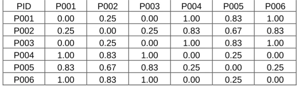
To calculate Jaccard coefficient of the pair P001 and P002, we first find out the number of item that are both coded as 1 is 3; and then the number of item that are either coded as 1 is 4. Therefore, the Jaccard coefficient = 1 – 3/4 = 0.25. For any pair of PID, the smaller the Jaccard coefficient indicates the more identical the pair is. Following this simple computation, the Jaccard coefficient of each pair of PID can be easily computed, and the example below expresses all 6 pairs of PID above in a square matrix:
PID P001 P002 P003 P004 P005 P006 P001 0.00 0.25 0.00 1.00 0.83 1.00 P002 0.25 0.00 0.25 0.83 0.67 0.83 P003 0.00 0.25 0.00 1.00 0.83 1.00 P004 1.00 0.83 1.00 0.00 0.25 0.00 P005 0.83 0.67 0.83 0.25 0.00 0.25 P006 1.00 0.83 1.00 0.00 0.25 0.00
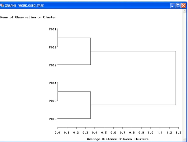
Hierarchical clustering builds a cluster hierarchy, or, in other words, a tree of clusters, which is also known as a dendrogram. Every cluster node contains child clusters; sibling clusters partition the points covered by their common parent. The agglomerative method (bottom-up hierarchical clustering approach) is applied to analyze the above data. It starts out with each data point forming its own cluster, and merges those two clusters that are nearest, to form a reduced number of clusters. This is repeated, each time merging the two closest clusters, until just one cluster, of all the data points, exists. There are various ways to determine the distance between clusters, and the one we used in this analysis is average linkage. The distance between two clusters is the average distance between all pairs of observations. Average linkage tends to join clusters with small variances, and it is slightly biased toward producing clusters with the same variance.
Figure 3.3. Dendrogram of the 6-patron sample dataset in Figure 3.1
the cluster fusion into only one (see appendix 8). These two statistics suggest the dataset consists of two clusters only; that is, P001 to P003 in cluster 1,
PID \ CallNo. QA1 QA2 QA3 HB1 HB2 HB3 P001 1 1 1 0 0 0 P002 1 1 1 0 1 0 P003 1 1 1 0 0 0
and P004 to P006 in cluster 2.
PID \ CallNo. QA1 QA2 QA3 HB1 HB2 HB3 P004 0 0 0 1 1 1 P005 0 1 0 1 1 1 P006 0 0 0 1 1 1
Following the same procedures on the simulated datasets 1 and 2, we will be able to create different clusters for each dataset.
LC Classification Method
PID \ CallNo. QA1 QA2 QA3 PID \ CallNo. HB1 HB2 HB3
P001 1 1 1 P002 0 1 0
P002 1 1 1 P004 1 1 1
P003 1 1 1 P005 1 1 1
P005 0 1 0 P006 1 1 1
Partition of QA Partition of HB
Notice that a patron may be showed up in more than one group if he/she has diversified interests in various subjects (like P002 and P005), while in clustering method, each patron can be assigned to one cluster only.
Again, following the same procedures on the simulated datasets 1 and 2, we will be able to create different partition for each dataset.
Association Discovery Rule
book B, book C) will be generated at the same time, while the third rule (book A => book B, book C) is in fact derived from the first rule (book A => book B) and second rule (book A => book C). In other words, the third rule is just a trivial rule. Therefore, to simplify our analysis, we simply allow single item in both antecedent and consequent.
Be aware that the rules should not be interpreted as a direct causation, but only interpreted as an association between two or more items. Association analysis does not create rules about repeating items; that is: it doesn't matter whether an individual patron borrow book A several time, only the presence of book A in the market basket is relevant.
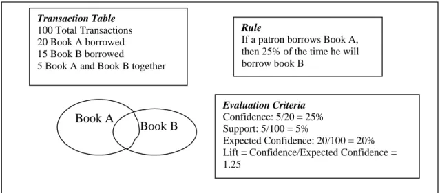
Figure 3.4 Diagram showing different terms in association rules
Since the SAS program will generate more than enough useful association rules if no constraint is defined, we have to set certain criteria before running the program. Creditable rules should have a large confidence factor, a large level of support, and a value of lift greater than one. Rules having a high level of confidence but little support should be interpreted with caution. Therefore, before applying association rules, we divide the whole dataset into different clusters to reduce the number of total transaction, thus improving the level of support. The association node in SAS enterprise program enables us to modify and control all the above selection criteria. Minimum transaction frequency to support association (in terms of percentage of the largest single item frequency) is set to 40%; minimum confidence for rule generation is set to 40% in our analysis; and number of count greater than 3. The code of SAS program for generating association rules is shown in appendix 9.
Transaction Table
100 Total Transactions 20 Book A borrowed 15 Book B borrowed
5 Book A and Book B together
Book A
Book B
Rule
If a patron borrows Book A, then 25% of the time he will borrow book B
Evaluation Criteria
Confidence: 5/20 = 25% Support: 5/100 = 5%
Chapter4: Results and Discussion
Results for Dataset 1:
Clustering Method
The tree diagram showing how different data point merges together is shown in Appendix 10. Since this dataset is constructed in a way of having three distinct clusters, the clustering method should generate the results as we expect. From appendix 11, the local peak of pseudo F is at three (F = 17.5), with a big jump of pseudo t2 (from 6.6 to 13.1) for the next cluster fusion. As a result, no further merging of clusters is needed when there are only three clusters left. Appendix 12 shows the resulting three clusters.
LC Classification
As we mentioned in the last chapter, the formation of different partitions is very straightforward. We form the partitions simply by grouping the patrons who borrow book within the same subject class, while discarding the circulation record outside that subject class. Three partitions for QA, PE and HB are formed and illustrated in appendix 13.
Comparison of Association Rules Generated from Clustering and LC Classification
when the dataset is segmented by using clustering method, while 75 association rules are produced when segmented by LC classification. 46 rules are overlapped. The average level of support and average level of confidence of all association rules in clustering case are 32.94% and 67.79%, while the average level of support and average level of confidence in LC classification case are 22.45% and 59.45%. Because patrons mostly borrow books within their favorite subject area, there is no cross subject recommendation generated from the association rules in both segmentation methods.
Results for Dataset 2:
Clustering Method
The tree diagram showing how different data point merges together is shown in appendix 16. Since this dataset is constructed in a way there is no clear borrowing pattern among patrons, the statistics that indicates when to stop merging the cluster is not as lucid as in Dataset 1. From appendix 17, the local peak of pseudo F is at five (F = 3.6), with a jump of pseudo t2 (from 2.0 to 4.3) for the next cluster fusion. The result indicates the best time to stop merging is when we have five clusters left. Appendix 18 shows the resulting five clusters.
LC Classification
Similar to the LC Classification method shown above, three partitions for QA, PE and HB are formed and illustrated in appendix 19.
The results of association rules generated from clustering and LC classification are shown in appendix 20 and 21 respectively. Totally, 103 association rules are generated when the dataset is segmented by using Clustering method, while 29 association rules are produced when segmented by LC classification. 10 rules are overlapped. The average level of support and average level of confidence of all the associations using clustering method are 36.87% and 70.53%, while the average level of support and average level of confidence using LC classification are 14.10% and 46.08%. Because patrons in this dataset have diversified interest in different subject areas, using clustering method to segment the dataset will result in association rules across different subject.
Which Segmentation Method Is Better, Clustering or LC Classification?
To evaluate our recommender system, we first have to figure what approaches are available to measure the performance. Konstan and Riedl suggest there are two categories of approaches to evaluate recommender systems: (1) Offline evaluation – where the performance is evaluated based on existing datasets. (2) Online evaluation – where performance is evaluated on users of a running recommender system. Since our recommender system is based on a simulated dataset that has never been launched to the general public, the online evaluation approach is not appropriate in evaluating our model. As a result, offline evaluation is the only approach for evaluating the performance.
Conclusion
Based on two simulated library circulation datasets, this paper compares clustering and LC classification to see which one is more desirable to segment the data for building up recommender systems. Despite the fact that association rules generated when using clustering method to segment the datasets yield higher level of support and confidence than those of LC classification. However, as we consider that the fact that it is difficult to form distinct clusters in reality, and patrons may switch their interests to different subject areas from time to time, using clustering method will yield a considerate number of irrelevant association rules. As a result, LC classification is preferable than clustering.
References
Agrawal, R., Imielinski, T., & Swami, A. (1993). Mining Association ruless Between Sets of Items in Large Databases. In P.Buneman and S.Jajordia, eds., Proceedings of the ACM Sigmoid International Conference on Management of Data, New York: ACM
Anderberg, M.R. (1973), Cluster Analysis for Applications, New York: Academic Press, Inc.
Association of Research Libraries. (2003). Service Trends in ARL Libraries, 1991-2002. Available at: http://www.arl.org/stats/arlstat/graphs/2002/2002t1.html
Balabanovic, M & Shaham, Y. (1997) Fab. Content-Based, Collaborative Recommendation, Communications of the ACM, 40(3), 66-72.
Ben-Dor, A. & Yakhini, Z. (1999). Clustering gene expression patterns. In Proceedings of the 2nd SIAM ICDM, 420-436, Arlington, VA.
Berkhin, P. (2002). Survey of clustering data mining techniques. Available: http://www.accrue.com/products/rp_cluster_review.pdf
Berson A., Smith S.J., & Kurt T. (2000). Building Data Mining Applications for CRM. New York: McGraw Hill.
Calinski, T. & Harabasz, J. (1974), A Dendrite Method for Cluster Analysis, Communications in Statistics, 3, 1 -27.
Cutting, D., Karger, D., Pedersen, J., & Tukey, J. (1992). Scatter/gather: a cluster-based approach to browsing large document collection. In Proceeding of the 15th ACM SIGIR Conference, 318-329, Copenhagen, Denmark.
Duda, R.O. & Hart, P.E. (1973). Pattern Classification and Scene Analysis, New York: John Wiley & Sons, NY.
Fayard, U.M., Piatetsky-Shapiro, G., Smyth, P. & Uthurusamy. R. (1996). Advances in Knowledge Discovery and Data Mining. Cambridge, MA: The MIT Press.
Han, J & Kamber, M. (2000). Data Mining: Concepts and Techniques. San Francisco : Morgan Kaufman Publishers.
Hand, D., Manila, H. & Smyth, P. (2001). Principles of Data Mining. Cambridge, MA: MIT Press.
Hayes, C. et al. An On-Line Evaluation Framework for Recommender Systems. Available at http://citeseer.nj.nec.com/552661.html
Heer, J. &Chi, E. (2001). Identification of Web user traffic composition using multi-modal clustering and information scent. In Proceedings of the 1st SIAM ICDM, Workshop on Web Mining, 51-58, Chicago, IL.
Hill, W. et al (1995). Recommending and evaluating choices in a virtual community of use." In: Conference on Human Factors in Computing Systems (CHI'95). Denver, May, 1995.
Jain, A.K. & Dubes, R.C. (1988). Algorithm for Clustering Data, Englewood Cliffs, NJ: Prentice Hall.
Klosgen, W & Zytkow, J.M. (2002). Handbook of Data Mining and Knowledge Discovery. New York: Oxford University Press.
Konstan, J.A. & Riedl, J. (1999). Research resources for recommender systems. In CHI’ 99 Workshop Interacting with Recommender Systems.
Kostan, J.A. et al (1997). GroupLens: applying collaborative filtering to usenet news.
Communications of the ACM. 40(3), 77-87.
Krulwich, B. & Burkey, C (1996). Learning user information interests through extraction of semantically significant phrases. In: Proceedings of the AAAI Spring Symposium on Machine Learning in Information Access. Stanford, California, March 1996.
Lang, K. (1995). Learning to filter news. In: Proceedings of the 12th International Conference on Machine Learning. Tahoe City, California, 1995.
Resnick, P & Varian, H.R. (1997) Recommender Systems. Communications of the ACM, 40(3), 56--58.
SAS lnc, (2002) SAS Technical Support Documents [Computer Software Manuel]. Available at http://www.sas.com/service/techsup/tnote/technote.html
Appendix 1: Catalog of 30 Books in the Library
LC Call Number Simplified Call Number
Title
PE1112 .L43 1996 PE1 An A-Z Of English Grammar And Usage PE1460 .T87 1995 PE2 ABC Of Common Grammatical Errors PE1112 .S73 1998 PE3 The Advanced Grammar Book PE1241 .A36 1992 PE4 Adjectives And Adverbs PE1111.L455
1956b
PE5 Better English
PE1112.H69 PE6 Brief Handbook For Writers
PE1112.W55 PE7 A Brief Handbook Of English With Research Paper PE1408.G934 PE8 Concise English Handbook
PE1408 .T6954 2001
PE9 The Contemporary Writer
PE1408 .K2725 1998
PE10 The Confident Writer
HB172.J44 HB1 Advanced Microeconomic Theory
HB172 .J44 2001 HB2 Advances In Self-Organization And Evolutionary Economics
HB172.C545 HB3 Applied Microeconomic Problems HB172.L56 HB4 Applied Price Theory
HB172.M39 1985 HB5 The Applied Theory Of Price HB172.5 .S5269
2001
HB6 An Introduction To Economic Dynamics
HB171.G185 HB7 Introduction To Microeconomic Theory.
HB172.I77 HB8 Issues In Contemporary Microeconomics And Welfare HB172.L43 1995 HB9 Learning And Rationality In Economics /
HB172.I77 HB10 Issues In Contemporary Microeconomics And Welfare QA76.64 .F74 1996 QA1 Active Java : Object-Oriented Programming For The World
Wide Web QA76.73.J38 D445
2002
QA2 Advanced Java 2 Platform : How To Program
QA76.73.J38 S75 1997
QA3 Advanced Java Networking
QA76.625 .S557 1998
QA4 The Complete Guide To Java Database Programming
QA76.642 .M343 1999
QA5 Concurrency : State Models & Java Programs
QA76.73.J38 H375 1998
QA6 Concurrent Programming : The Java Programming Language
QA76.73.J38 H345 2000
QA7 Core Servlets And JavaServer Pages
QA76.9.D343 W58 2000
QA8 Data Mining : Practical Machine Learning Tools And Techniques
QA76.9.U83 T66 2000
QA9 Core Swing : Advanced Programming
QA76.73.J38 E44 2000
Appendix 2. Sample Circulation Record
PID Call No CheckOut Return
Appendix 3: Macro Program that Generates Dataset 1 Sub Macro5()
' This program generate the first dataset
ActiveCell.Cells.Select
Selection.NumberFormat = "General"
Randomize
' i represent the number of patron, j represent the number of books For i = 2 To 61
For j = 2 To 31
' assign the first 20 patron frequently read the first 10 books, next 20
' patrons frequently
' to read the next 20 books, and last 20 patrons to last 10 books
If (i <= 20 And j <= 10) Or (i > 20 And i <= 40 And j > 10 And j <= 20) Or
(i > 40 And i <= 60 And j > 20 And j <= 30) Then If Rnd > 0.15 Then
Cells(i, j).Value = 1 Else
Cells(i, j).Value = 0 End If
' patrons fallen out from the interested book area have low circulation ' record
Else
If Rnd > 0.95 Then
Cells(i, j).Value = 1 Else
Cells(i, j).Value = 0 End If
End If
Next j
Next i
Appendix 4: Macro Program that Generates Dataset 2 Sub Macro5()
' This program generate the second dataset
ActiveCell.Cells.Select
Selection.NumberFormat = "General"
Randomize
' i represent the number of patron, j represent the number of books For i = 1 To 61
For j = 1 To 31
' everybody got equal chance (0.7) to borrow a book If Rnd > 0.3 Then
Cells(i, j).Value = 1 Else
Cells(i, j).Value = 0 End If
Next j
Next i
Appendix 6: Macro Program Converting Circulation Data Sub Macro1()
'
' Macro1 Macro
' Macro recorded 10/18/2003 by ATN
' This program is to convert the circulation record format for clustering into an orderly
' circulation record. One has to change the No_of_patron and No_of_book accordingly
' before running the program.
No_of_patron = 60 No_of_book = 30 Target = "Sheet3" Origin = "Sheet2"
I = 1 K = 1
Do While I <= No_of_patron + 1 J = 1
Do While J <= No_of_book + 1 Sheets(Origin).Select
If Cells(I + 1, J + 1) = 1 Then
Cells(I + 1, 1).Select Selection.Copy
Sheets(Target).Select Cells(K + 1, 1).Select ActiveSheet.Paste Sheets(Origin).Select Cells(1, J + 1).Select Selection.Copy
Sheets(Target).Select Cells(K + 1, 2).Select ActiveSheet.Paste K = K + 1
End If J = J + 1 Loop
I = I + 1 Loop
Appendix 7: SAS program for Clustering Method
%include 'd:/libthesis2/xmacro.sas'; %include 'd:/libthesis2/distnew.sas'; options ls=120 ps=60;
proc print data=cluster; run;
%distance(data=CLUSTER, id=PID, options=nomiss, out=distjacc, shape=square, method=djaccard, var=QA1--HB10); proc print data=distjacc(obs=10);
id PID; var P001-P060;
title2 'Jaccard Coefficient of 60 users'; run;
title2;
proc cluster data=distjacc method=average pseudo outtree=tree;
id PID;
var P001-P060; run;
proc tree graphics horizontal; run;
proc tree data=tree noprint n=3 out=out; id PID; run; proc sort; by PID; run; data clus;
Appendix 8: The Statistical Output of Cluster Procedure for the sample dataset The SAS System
The CLUSTER Procedure Average Linkage Cluster Analysis
Root-Mean-Square Distance Between Observations = 0.705796
Cluster History
Appendix 9: SAS Program for Generating Association Rules
Appendix 10: Tree Diagram Showing How Data Points Merge Together for Dataset 1
Appendix 11: The Statistical Output of Cluster Procedure for Dataset 1
The SAS System 06:19 Wednesday, December 10, 2003 5
The CLUSTER Procedure Average Linkage Cluster Analysis
Root-Mean-Square Distance Between Observations = 0.895693
Cluster History
Norm T
Appendix 12: Clustering Method Results for Dataset 1 Cluster 1
Cluster 2:
Appendix 13: LC Classification Method Results for Dataset 1
Partition for QA Partition for PE Partition for HB
Appendix 14: Association Rules for Dataset 1 Using Clustering to Segment the Data
CLUSTER RULE CONF SUPPORT LIFT COUNT EXP_CONF
1.00 QA4 ==> QA2 80.00 40.00 1.60 8.00 50.00 1.00 QA2 ==> QA4 80.00 40.00 1.60 8.00 50.00 1.00 QA9 ==> QA3 100.00 30.00 2.00 6.00 50.00 1.00 QA3 ==> QA9 60.00 30.00 2.00 6.00 30.00 1.00 QA7 ==> QA1 50.00 30.00 1.25 6.00 40.00 1.00 QA1 ==> QA7 75.00 30.00 1.25 6.00 60.00 1.00 QA10 ==> QA1 60.00 30.00 1.50 6.00 40.00 1.00 QA1 ==> QA10 75.00 30.00 1.50 6.00 50.00 1.00 QA8 ==> QA3 62.50 25.00 1.25 5.00 50.00 1.00 QA3 ==> QA8 50.00 25.00 1.25 5.00 40.00 1.00 QA3 ==> QA1 50.00 25.00 1.25 5.00 40.00 1.00 QA1 ==> QA3 62.50 25.00 1.25 5.00 50.00 1.00 QA9 ==> QA7 66.67 20.00 1.11 4.00 60.00 1.00 QA9 ==> QA10 66.67 20.00 1.33 4.00 50.00 1.00 QA10 ==> QA9 40.00 20.00 1.33 4.00 30.00 1.00 QA8 ==> QA6 50.00 20.00 1.67 4.00 30.00 1.00 QA6 ==> QA8 66.67 20.00 1.67 4.00 40.00 1.00 QA8 ==> QA1 50.00 20.00 1.25 4.00 40.00 1.00 QA1 ==> QA8 50.00 20.00 1.25 4.00 40.00 1.00 QA6 ==> QA7 66.67 20.00 1.11 4.00 60.00 1.00 QA5 ==> QA7 100.00 20.00 1.67 4.00 60.00 1.00 QA6 ==> QA4 66.67 20.00 1.33 4.00 50.00 1.00 QA4 ==> QA6 40.00 20.00 1.33 4.00 30.00 1.00 QA6 ==> QA2 66.67 20.00 1.33 4.00 50.00 1.00 QA2 ==> QA6 40.00 20.00 1.33 4.00 30.00 1.00 QA5 ==> QA3 100.00 20.00 2.00 4.00 50.00 1.00 QA3 ==> QA5 40.00 20.00 2.00 4.00 20.00
AVERAGE 63.52 24.44 1.46 4.89 44.07
2.00 PE6 ==> PE2 75.00 42.86 1.43 9.00 52.38 2.00 PE2 ==> PE6 81.82 42.86 1.43 9.00 57.14 2.00 PE4 ==> PE10 100.00 42.86 1.50 9.00 66.67 2.00 PE10 ==> PE4 64.29 42.86 1.50 9.00 42.86 2.00 PE7 ==> PE2 66.67 38.10 1.27 8.00 52.38 2.00 PE2 ==> PE7 72.73 38.10 1.27 8.00 57.14 2.00 PE8 ==> PE4 77.78 33.33 1.81 7.00 42.86 2.00 PE4 ==> PE8 77.78 33.33 1.81 7.00 42.86 2.00 PE4 ==> PE1 77.78 33.33 1.02 7.00 76.19 2.00 PE1 ==> PE4 43.75 33.33 1.02 7.00 42.86 2.00 PE9 ==> PE7 60.00 28.57 1.05 6.00 57.14 2.00 PE7 ==> PE9 50.00 28.57 1.05 6.00 47.62 2.00 PE9 ==> PE6 60.00 28.57 1.05 6.00 57.14 2.00 PE6 ==> PE9 50.00 28.57 1.05 6.00 47.62 2.00 PE9 ==> PE2 60.00 28.57 1.15 6.00 52.38 2.00 PE2 ==> PE9 54.55 28.57 1.15 6.00 47.62
AVERAGE 72.08 40.63 1.26 8.53 57.62
3.00 HB8 ==> HB2 90.00 45.00 1.29 9.00 70.00 3.00 HB2 ==> HB8 64.29 45.00 1.29 9.00 50.00 3.00 HB5 ==> HB2 80.00 40.00 1.14 8.00 70.00 3.00 HB2 ==> HB5 57.14 40.00 1.14 8.00 50.00 3.00 HB9 ==> HB8 60.00 30.00 1.20 6.00 50.00 3.00 HB8 ==> HB9 60.00 30.00 1.20 6.00 50.00 3.00 HB7 ==> HB4 54.55 30.00 1.36 6.00 40.00 3.00 HB4 ==> HB7 75.00 30.00 1.36 6.00 55.00 3.00 HB6 ==> HB10 100.00 30.00 1.54 6.00 65.00 3.00 HB10 ==> HB6 46.15 30.00 1.54 6.00 30.00 3.00 HB3 ==> HB10 85.71 30.00 1.32 6.00 65.00 3.00 HB10 ==> HB3 46.15 30.00 1.32 6.00 35.00 3.00 HB7 ==> HB3 45.45 25.00 1.30 5.00 35.00 3.00 HB3 ==> HB7 71.43 25.00 1.30 5.00 55.00
AVERAGE 66.85 32.86 1.31 6.57 51.43
Appendix 15: Association Rules for Dataset 1 Using LC Classification to Segment the Data
PARTITON RULE CONF SUPPORT LIFT COUNT EXP_CONF
QA QA4 ==> QA2 66.67 23.53 2.06 8.00 32.35
QA QA2 ==> QA4 72.73 23.53 2.06 8.00 35.29
QA QA9 ==> QA3 100.00 17.65 2.62 6.00 38.24
QA QA3 ==> QA9 46.15 17.65 2.62 6.00 17.65
QA QA7 ==> QA3 46.15 17.65 1.21 6.00 38.24
QA QA3 ==> QA7 46.15 17.65 1.21 6.00 38.24
QA QA7 ==> QA10 46.15 17.65 1.43 6.00 32.35
QA QA10 ==> QA7 54.55 17.65 1.43 6.00 38.24
QA QA7 ==> QA1 46.15 17.65 1.74 6.00 26.47
QA QA1 ==> QA7 66.67 17.65 1.74 6.00 38.24
QA QA10 ==> QA1 54.55 17.65 2.06 6.00 26.47
QA QA1 ==> QA10 66.67 17.65 2.06 6.00 32.35
QA QA8 ==> QA3 45.45 14.71 1.19 5.00 38.24
QA QA10 ==> QA3 45.45 14.71 1.19 5.00 38.24
QA QA1 ==> QA3 55.56 14.71 1.45 5.00 38.24
AVERAGE 57.27 17.84 1.74 6.07 33.92
PE PE10 ==> PE1 80.00 37.50 1.60 12.00 50.00 PE PE1 ==> PE10 75.00 37.50 1.60 12.00 46.88 PE PE3 ==> PE1 61.11 34.38 1.22 11.00 50.00 PE PE1 ==> PE3 68.75 34.38 1.22 11.00 56.25 PE PE9 ==> PE3 100.00 31.25 1.78 10.00 56.25 PE PE3 ==> PE9 55.56 31.25 1.78 10.00 31.25 PE PE7 ==> PE3 83.33 31.25 1.48 10.00 56.25 PE PE3 ==> PE7 55.56 31.25 1.48 10.00 37.50 PE PE7 ==> PE10 83.33 31.25 1.78 10.00 46.88 PE PE10 ==> PE7 66.67 31.25 1.78 10.00 37.50 PE PE6 ==> PE1 58.82 31.25 1.18 10.00 50.00 PE PE1 ==> PE6 62.50 31.25 1.18 10.00 53.13 PE PE8 ==> PE10 90.00 28.13 1.92 9.00 46.88 PE PE10 ==> PE8 60.00 28.13 1.92 9.00 31.25
PE PE8 ==> PE1 90.00 28.13 1.80 9.00 50.00
PE PE1 ==> PE8 56.25 28.13 1.80 9.00 31.25
PE PE6 ==> PE2 52.94 28.13 1.41 9.00 37.50
PE PE2 ==> PE6 75.00 28.13 1.41 9.00 53.13
PE PE6 ==> PE10 52.94 28.13 1.13 9.00 46.88 PE PE10 ==> PE6 60.00 28.13 1.13 9.00 53.13 PE PE4 ==> PE10 100.00 28.13 2.13 9.00 46.88 PE PE10 ==> PE4 60.00 28.13 2.13 9.00 28.13 PE PE3 ==> PE10 50.00 28.13 1.07 9.00 46.88 PE PE10 ==> PE3 60.00 28.13 1.07 9.00 56.25
PE PE2 ==> PE7 66.67 25.00 1.78 8.00 37.50
PE PE7 ==> PE1 66.67 25.00 1.33 8.00 50.00
PE PE1 ==> PE7 50.00 25.00 1.33 8.00 37.50
PE PE3 ==> PE2 44.44 25.00 1.19 8.00 37.50
PE PE2 ==> PE3 66.67 25.00 1.19 8.00 56.25
PE PE8 ==> PE4 70.00 21.88 2.49 7.00 28.13
PE PE4 ==> PE8 77.78 21.88 2.49 7.00 31.25
PE PE4 ==> PE1 77.78 21.88 1.56 7.00 50.00
PE PE1 ==> PE4 43.75 21.88 1.56 7.00 28.13
PE PE2 ==> PE10 58.33 21.88 1.24 7.00 46.88 PE PE10 ==> PE2 46.67 21.88 1.24 7.00 37.50
PE PE2 ==> PE1 58.33 21.88 1.17 7.00 50.00
PE PE1 ==> PE2 43.75 21.88 1.17 7.00 37.50
AVERAGE 65.66 27.80 1.54 8.89 43.83
HB HB8 ==> HB2 75.00 29.03 1.45 9.00 51.61
HB HB2 ==> HB8 56.25 29.03 1.45 9.00 38.71
HB HB5 ==> HB2 72.73 25.81 1.41 8.00 51.61
HB HB2 ==> HB5 50.00 25.81 1.41 8.00 35.48
HB HB2 ==> HB10 50.00 25.81 1.03 8.00 48.39 HB HB10 ==> HB2 53.33 25.81 1.03 8.00 51.61
HB HB9 ==> HB2 70.00 22.58 1.36 7.00 51.61
HB HB2 ==> HB9 43.75 22.58 1.36 7.00 32.26
HB HB9 ==> HB8 60.00 19.35 1.55 6.00 38.71
HB HB8 ==> HB9 50.00 19.35 1.55 6.00 32.26
HB HB8 ==> HB10 50.00 19.35 1.03 6.00 48.39 HB HB10 ==> HB8 40.00 19.35 1.03 6.00 38.71
HB HB7 ==> HB4 50.00 19.35 1.72 6.00 29.03
HB HB4 ==> HB7 66.67 19.35 1.72 6.00 38.71
HB HB7 ==> HB10 50.00 19.35 1.03 6.00 48.39 HB HB10 ==> HB7 40.00 19.35 1.03 6.00 38.71 HB HB6 ==> HB10 100.00 19.35 2.07 6.00 48.39 HB HB10 ==> HB6 40.00 19.35 2.07 6.00 19.35 HB HB5 ==> HB10 54.55 19.35 1.13 6.00 48.39 HB HB10 ==> HB5 40.00 19.35 1.13 6.00 35.48 HB HB3 ==> HB10 66.67 19.35 1.38 6.00 48.39 HB HB10 ==> HB3 40.00 19.35 1.38 6.00 29.03
AVERAGE 55.41 21.70 1.38 6.73 41.06
Total Average 59.45 22.45 1.55 7.23 39.60
Appendix 17: The Statistical Output of Cluster Procedure for Dataset 2 The SAS System 02:29 Wednesday, December 10, 2003 5
The CLUSTER Procedure Average Linkage Cluster Analysis
Root-Mean-Square Distance Between Observations = 0.831392
Cluster History
Appendix 18: Clustering Method Results for Dataset 2 Cluster 1:
Cluster 2:
Cluster 3:
Cluster 4:
Appendix 19: LC Classification Method Results for Dataset 2
Partition for QA Partition for PE Partition for HB
Appendix 20: Association Rules for Dataset 2 Using Clustering to Segment the Data
CLUSTER RULE CONF SUPPORT LIFT COUNT EXP_CONF
1.00 PE6 ==> PE7 42.86 25.00 1.14 6.00 37.50 1.00 HB1 ==> HB7 75.00 25.00 1.13 6.00 66.67
AVERAGE 61.05 28.33 1.21 6.80 50.74
2.00 PE3 ==> PE2 66.67 57.14 1.04 8.00 64.29 2.00 PE2 ==> PE3 88.89 57.14 1.04 8.00 85.71 2.00 PE3 ==> HB8 58.33 50.00 1.02 7.00 57.14 2.00 HB8 ==> PE3 87.50 50.00 1.02 7.00 85.71 2.00 QA5 ==> QA1 75.00 42.86 1.05 6.00 71.43 2.00 QA1 ==> QA5 60.00 42.86 1.05 6.00 57.14 2.00 QA8 ==> PE2 100.00 35.71 1.56 5.00 64.29 2.00 PE2 ==> QA8 55.56 35.71 1.56 5.00 35.71 2.00 QA7 ==> QA1 100.00 35.71 1.40 5.00 71.43 2.00 QA1 ==> QA7 50.00 35.71 1.40 5.00 35.71 2.00 QA1 ==> HB3 50.00 35.71 1.40 5.00 35.71 2.00 HB3 ==> QA1 100.00 35.71 1.40 5.00 71.43 2.00 QA9 ==> QA5 80.00 28.57 1.40 4.00 57.14 2.00 QA5 ==> QA9 50.00 28.57 1.40 4.00 35.71 2.00 QA9 ==> QA1 80.00 28.57 1.12 4.00 71.43 2.00 QA1 ==> QA9 40.00 28.57 1.12 4.00 35.71 2.00 QA8 ==> QA1 80.00 28.57 1.12 4.00 71.43 2.00 QA1 ==> QA8 40.00 28.57 1.12 4.00 35.71 2.00 QA7 ==> PE1 80.00 28.57 2.24 4.00 35.71 2.00 PE1 ==> QA7 80.00 28.57 2.24 4.00 35.71 2.00 QA5 ==> QA10 50.00 28.57 1.17 4.00 42.86 2.00 QA10 ==> QA5 66.67 28.57 1.17 4.00 57.14 2.00 QA5 ==> PE1 50.00 28.57 1.40 4.00 35.71 2.00 PE1 ==> QA5 80.00 28.57 1.40 4.00 57.14 2.00 QA5 ==> HB1 50.00 28.57 1.40 4.00 35.71 2.00 HB1 ==> QA5 80.00 28.57 1.40 4.00 57.14 2.00 QA10 ==> PE2 66.67 28.57 1.04 4.00 64.29 2.00 PE2 ==> QA10 44.44 28.57 1.04 4.00 42.86 2.00 QA1 ==> PE1 40.00 28.57 1.12 4.00 35.71 2.00 PE1 ==> QA1 80.00 28.57 1.12 4.00 71.43 2.00 PE5 ==> PE3 100.00 28.57 1.17 4.00 85.71 2.00 HB7 ==> PE3 100.00 28.57 1.17 4.00 85.71 2.00 HB6 ==> PE3 100.00 28.57 1.17 4.00 85.71 2.00 PE2 ==> HB1 44.44 28.57 1.24 4.00 35.71 2.00 HB1 ==> PE2 80.00 28.57 1.24 4.00 64.29
AVERAGE 70.12 33.47 1.28 4.69 56.33
3.00 PE1 ==> PE10 66.67 44.44 1.50 4.00 44.44
AVERAGE 76.67 44.44 1.30 4.00 59.26
4.00 PE4 ==> PE1 71.43 50.00 1.02 5.00 70.00 4.00 PE1 ==> PE4 71.43 50.00 1.02 5.00 70.00 4.00 QA7 ==> QA2 100.00 40.00 2.00 4.00 50.00 4.00 QA2 ==> QA7 80.00 40.00 2.00 4.00 40.00 4.00 QA5 ==> PE4 80.00 40.00 1.14 4.00 70.00 4.00 PE4 ==> QA5 57.14 40.00 1.14 4.00 50.00 4.00 QA5 ==> PE1 80.00 40.00 1.14 4.00 70.00 4.00 PE1 ==> QA5 57.14 40.00 1.14 4.00 50.00 4.00 QA2 ==> PE4 80.00 40.00 1.14 4.00 70.00 4.00 PE4 ==> QA2 57.14 40.00 1.14 4.00 50.00 4.00 PE7 ==> PE5 80.00 40.00 1.60 4.00 50.00 4.00 PE5 ==> PE7 80.00 40.00 1.60 4.00 50.00 4.00 PE5 ==> PE1 80.00 40.00 1.14 4.00 70.00 4.00 PE1 ==> PE5 57.14 40.00 1.14 4.00 50.00 4.00 PE4 ==> HB3 57.14 40.00 1.43 4.00 40.00 4.00 HB3 ==> PE4 100.00 40.00 1.43 4.00 70.00
AVERAGE 74.29 41.25 1.33 4.13 57.50
Appendix 21: Association Rules for Dataset 2 Using LC classification to Segment the Data
PARTITION RULE CONF SUPPORT LIFT COUNT EXP_CONF
QA QA8 ==> QA6 50.00 18.33 1.88 11.00 26.67
QA QA6 ==> QA8 68.75 18.33 1.88 11.00 36.67
QA QA8 ==> QA1 50.00 18.33 1.36 11.00 36.67
QA QA1 ==> QA8 50.00 18.33 1.36 11.00 36.67
QA QA10 ==> QA1 47.62 16.67 1.30 10.00 36.67 QA QA1 ==> QA10 45.45 16.67 1.30 10.00 35.00
QA QA7 ==> QA10 47.37 15.00 1.35 9.00 35.00
QA QA10 ==> QA7 42.86 15.00 1.35 9.00 31.67
QA QA4 ==> QA10 50.00 15.00 1.43 9.00 35.00
QA QA10 ==> QA4 42.86 15.00 1.43 9.00 30.00
QA QA4 ==> QA1 50.00 15.00 1.36 9.00 36.67
QA QA1 ==> QA4 40.91 15.00 1.36 9.00 30.00
QA QA7 ==> QA8 42.11 13.33 1.15 8.00 36.67
QA QA7 ==> QA2 42.11 13.33 1.40 8.00 30.00
QA QA2 ==> QA7 44.44 13.33 1.40 8.00 31.67
QA QA7 ==> QA1 42.11 13.33 1.15 8.00 36.67
QA QA6 ==> QA1 50.00 13.33 1.36 8.00 36.67
QA QA5 ==> QA2 40.00 13.33 1.33 8.00 30.00
QA QA2 ==> QA5 44.44 13.33 1.33 8.00 33.33
QA QA5 ==> QA1 40.00 13.33 1.09 8.00 36.67
AVERAGE 46.55 15.17 1.38 9.10 33.92
PE PE9 ==> PE6 42.11 13.33 1.20 8.00 35.00
PE PE3 ==> PE2 61.54 13.33 2.17 8.00 28.33
PE PE2 ==> PE3 47.06 13.33 2.17 8.00 21.67
PE PE2 ==> PE1 47.06 13.33 1.28 8.00 36.67
AVERAGE 49.44 13.33 1.71 8.00 30.42
HB HB8 ==> HB7 42.11 13.79 1.11 8.00 37.93
HB HB8 ==> HB1 42.11 13.79 1.22 8.00 34.48
HB HB1 ==> HB8 40.00 13.79 1.22 8.00 32.76
HB HB10 ==> HB1 47.06 13.79 1.36 8.00 34.48
HB HB1 ==> HB10 40.00 13.79 1.36 8.00 29.31
AVERAGE 42.25 13.79 1.26 8.00 33.79