Development of an Efficient Face Recognition System Based on Linear and Nonlinear Algorithms

ISSN: 2252-8938  80

Development of an Efficient Face Recognition System Based on

Linear and Nonlinear Algorithms

Federal University of Technology, Akure, Ondo State, Nigeria

Article Info ABSTRACT

Article history: Received Mar 6, 2016 Revised May 10, 2016 Accepted May 27, 2016

This paper presents appearance based methods for face recognition using linear and nonlinear techniques. The linear algorithms used are Principal Component Analysis (PCA) and Linear Discriminant Analysis (LDA). The two nonlinear methods used are the Kernel Principal Components Analysis (KPCA) and Kernel Fisher Analysis (KFA). The linear dimensional reduction projection methods encode pattern information based on second order dependencies. The nonlinear methods are used to handle relationships among three or more pixels. In the final stage, Mahalinobis Cosine (MAHCOS) metric is used to define the similarity measure between two images after they have passed through the corresponding dimensional reduction techniques. The experiment showed that LDA and KFA have the highest performance of 93.33 % from the CMC and ROC results when used with Gabor wavelets. The overall result using 400 images of AT&T database showed that the performance of the linear and nonlinear algorithms can be affected by the number of classes of the images, preprocessing of images, and the number of face images of the test sets used for recognition.

Keyword:

Appearance-Based Methods Dimensional Reduction Techniques

Face Recognition Gabor Wavelets

Linear And Nonlinear Face Recognition Algorithms

Copyright © 2016 Institute of Advanced Engineering and Science. All rights reserved. Corresponding Author:

Araoluwa Simileolu Filani,

Teaching Assistant, Department of Computer Science,

Federal University of Technology, Akure, Ondo State, Nigeria. Email: [email protected]

1. INTRODUCTION

The development of the robust recognition system is a very important area under discussion because of the wide range of applications in different spheres, such as video surveillance security systems, control of documents, forensics systems etc. [1]. In the last three decades face identification problem has emerged as an important research area with many possible applications that undoubtedly alleviate and assist safeguard our everyday lives in many aspects [2]. Unlike many other identification methods, face recognition does not need to make direct contact with an individual in order to validate their identity. This can be useful for surveillance or tracking and in detection systems. Data acquisition in general is fraught with problems for other biometrics: techniques that rely on hands and fingers can be rendered useless if the epidermis tissue is injured in some way (i.e., bruised or cracked). Although there are a number of face recognition algorithms which work well in constrained environments, face recognition is still an open and difficult problem in real applications [3].

In face recognition, appearance-based approach has been widely used [4]. The Face images often have a large number of pixel values and are represented as high-dimensional vectors or arrays. Operating directly on these vectors is inefficient, would lead to high computational costs and storage space, and poses the curse of dimensionality to many learning tasks. A useful subspace representation has thus become desirable in many image processing applications. The holistic and component-based methods are two main ways for representing the facial appearances. Compared to holistic approaches, feature-based methods are less sensitive to variations in illumination and viewpoint [2]. In holistic representation, a facial image is

considered as a vector of pixels and is represented as a single point in the high dimensional space. Subspace methods are then applied to reduce the high-dimensional data onto a lower dimensional space while retaining intrinsic features for further classification [5], [6]. The holistic appearance based methods can be classified as linear methods and nonlinear methods. Linear methods explicitly transform data from high dimensional subspace into low dimensional subspace by linear mapping. In nonlinear techniques, explicit projections are not done. Instead faithful low dimensional data matrix is obtained directly from high dimensional data matrix. The successful face linear or nonlinear methods used depends heavily on the particular choice of the features used by the pattern classifier. Therefore, detailed evaluation and benchmarking of the algorithms is crucial for later use.

Appearance face recognition methods do not perform well during ill conditions [2], [7], even the most representative recognition techniques frequently used in conjunction with face recognition could not achieve best result [7], [8]. One of the most successful classifiers that has been used for image representation is Gabor Wavelets. This is because it is a very strong preprocessing and extraction algorithms [9], [10], [11]. In this regard Gabor Wavelets is chosen for this work to provide robust face recognition algorithms. The remaining parts of this paper are organized as follows: Section II gives a review of face recognition methodologies. Section III describes the methodology of this work. Section IV presents the experiments and the results. Finally, the conclusion of the work is drawn in section V.

2. RELATED STUDIES

A major issue of face recognition is how to improve the overall performance of the employed recognition techniques [12], [13]. Most of the previous methods were mainly focused on frontal face images or single-view-based face recognition. The problem with these early solutions was the manual computations of features measurements and locations [14]. The notable earliest approaches in is the Eigenfaces [2]. The eigenfaces techiques was developed by Sirovich and Kirby (1987) and used by Matthew Turk and Alex Pentland in face classification [13], [15] by using standard linear algebra technique. An N×N image I is linearized in a 𝑁2 _{vector, so that it represents a point in a 𝑁}2_{-dimensional space. Recognition of a probe}

image is performed in a lower dimensional space by means of a dimensionality reduction technique using PCA (Principal Component Analysis). After the linearization the mean vector is calculated. The covariance matrix is then computed, in order to extract a limited number of its eigenvectors, corresponding to the greatest eigenvalues called eigenfaces. As the PCA is performed only for training the system, this technique appears to be very fast when testing new face images. The PCA has been intensively exploited in face recognition applications, and many of its variations have been developed. Many other linear projection methods that performed better under some conditions have been studied. The LDA (Linear Discriminant Analysis) [6] has been developed as a better technique than PCA. When compared with PCA, LDA gives a higher recognition rate when a wide training set is available. To provide a stronger system, PCA has been combined with LDA [16] but it has been shown in [17] that, combining PCA and LDA, cannot always produced desired result. ICA was introduced for providing face representations with high-order dependencies that are separated into individual coefficients and was expected to give superior recognition performance than PCA which only depend on separate second-order redundancies [18]. Afterwards, ICA theory was contradictory, and it has been shown that ICA does not always perform better then PCA or just suitable for a specific task [19], [20]. To overcome some of the limitations of the mentioned, other hybrids of PCA, LDA and ICA algorithms were develped. Most of these newer techniques involve combination of one or more algorithms [8], [21], [6].

As a PCA and LDA fail to discover the underlying structure of face images that lie on a hidden nonlinear submanifold, a laplacianface approach was proposed in [22] to provide a method that could detect the underlying structure of faces that lie on a hidden nonlinear submainfold that PCA and LDA could not discover. During the training stage, the images were first projected to a PCA subspace so that the resulting singular matrix is nonsingular. Egenvectors and Eigenvalues were then constructed for the generalized eigenvector problem so that the linear mapping best preserves the manifold’s estimated intrinsic geometry in a linear sense. The Laplacianfaces method is based on Locality Preserving Projections (LPP) which is a linear method and may not detect all aspects of the intrinsic nonlinear manifold structure by preserving local structure. A novel approach based on Two-dimensional Principal Component Analysis (2DPCA) and Kernel Principal Component Analysis (KPCA) for face recognition was developed in [23]. The work first performs Two-dimensional Principal Component Analysis process to project the faces onto the feature space. It then performs Kernel Principal Component Analysis on the projected data. Although it showed that the system achieved a high recognition rate, it only focused on Principal Component Analysis improved techniques that maximizes global variance for compression and not for classification like LDA. Thus the system will performed worse for system having high number of classes of images. A Face Recognition algorithm with

Support Vector Machines (SVM) was presented in [24]. The paper provided a face identification system based on SVM and Discrete Wavelet Transform (DWT). The DWT was used to avoid increase in the computational time. However it has been shown that nonlinear vector like SVM that do not always performed better than linear methods in real-world data sets having more complicated distributions, though they easily demonstrate their virtue on artificial nonlinear data [5]. Face Recognition System Based on Principal Component Analysis (PCA) with Back Propagation Neural Networks (BPNN) was developed in [25]. Support Vector Machine was used for face recognition. Similarly, in [26], BPNN was used. The features of the query face image and database face images was extracted using Gabor transform and trained using BPNN. Generally, neural network are nonlinear methods that encounter problems when the number of classes increases are not suitable for a single model image recognition task [21]. This paper involves the use of Gabor Wavelet for image representation with linear and non linear techniques, namely, PCA, LDA, KPCA and KFA and also studies the result of the same algorithms without the use of Gabor image representation.

3. METHODOLOGY

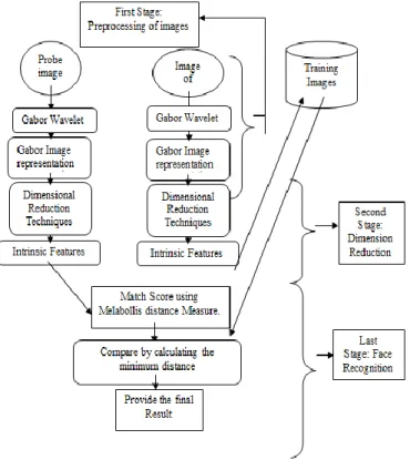
Figure 1 show the Frame work used. The first stage is the preprocessing stage. The preprocessing representation addresses image variabilities caused by illumination, facial expression and other different image imperfections. This was achieved by the integration of Gabor wavelet for extraction process to form the Gabor image representation of the images. The Gabor wavelets (kernels, filters) used is defined as shown in Equation (1)

𝜑𝑛,𝑏(z) = ‖𝑘𝑛,𝑏‖2

𝜎2 𝑒

−‖𝑘𝑛,𝑏‖

2 ‖𝑧‖2

2𝜎2 [𝑒𝑖𝑘𝑛,𝑏𝑧_{− 𝑒}− 𝜎2

2] ₍₁₎

where 𝑛 and b define the orientation and scale of the Gabor kernels, 𝑧 = (𝑥, 𝑦), ‖. ‖ denotes the norm operator, and the wave vector 𝑘𝑛,𝑏 is defined as follows:

𝑘𝑛,𝑏 = 𝑘𝑏𝑒𝑖∅𝑛 (2)

where 𝑘𝑏 = 𝑘𝑚𝑎𝑥 / 𝑓𝑏 and ∅𝑛= 𝜋𝑛/ 8. 𝑘𝑚𝑎𝑥 is the maximum frequency, and f is the spacing factor between

kernels in the frequency domain. The effect of the difference of convex functions term becomes negligible when the parameter 𝜎, which determines the ratio of the Gaussian window width to wavelength, has sufficiently large values. As in most cases Gabor wavelets used is of five different scales, 𝑏 ϵ {0, … ,4}, and eight orientations, 𝑛 ϵ {0, … ,7} [27].

For the Gabor feature representation, the Gabor wavelet representation of an image is the convolution of the image with the family of Gabor kernels as defined by (1). Let I(x,y) be the gray-level distribution of an image, the convolution of image I is defined as follows:

𝑂𝑛,𝑏(𝑧) = I (z) * 𝜑𝑛,𝑏(𝑧) (3)

where the following counts 𝑧 = (𝑥, 𝑦), ∗ denotes the convolution operator, and 𝑂𝑛,𝑏 (𝑧) is the convolution

result corresponding to the Gabor kernel at orientation 𝑛 and scale 𝑏. Which produce the set

S = {𝑂𝑛,𝑏(𝑧): 𝑛 ∈ {0, … ,7}, 𝑏 ∈ {0, … ,4}} (4)

Equation (4) forms the Gabor wavelet representation of the image I (z). To encompass different spatial frequencies (scale), spatial localities, and orientation selectivites, all the respresentation results are concatenated and an augmented feature vector X is derived by downsampling [26], [28].

The dimension of Gaborfaces is very high. In order to reduce the dimensionality, at the same time reserve the intrinsic part of the images, the dimensional reduction techniques were used in the second stage. After passing through the preprocessing stages, the trained images undergo dimensional reduction processes using the linear and the nonlinear techniques: PCA, LDA, KPCA and KFA by projecting the images onto subspace and storing their projections in the database. Also, before the matching, the probe images are preprocessed, and projected onto the same subspace as the gallery image using a similar algorithm. The final stage is the recognition stage.

The test image projections is then compared to stored gallery projections by using Mahalanobis Cosine distance metric by calculating the distances from a probe image projection to all gallery images projections and then choosing the minimum distance as a similarity measure. The identity of the most similar gallery image is then chosen to be the result of recognition and the unknown probe image is identified. The dataset are from the AT&T face database. There are 400 images in all. There are 40 datasets containing different subjects. Each datasets has 10 samples. The first three samples are selected for training, the next four samples were preserved as the test set, the remaining samples were used as the evaluating set. The algorithms used are described in the next section.

3.1. Principal Component Analysis (PCA)

Principal Component Analysis (PCA) is used to linearly separate the image vectors into a lower data. If v-dimensional vector of each training face of set has M images, the Principal Component Analysis (PCA) algorithm is used to find a t-dimensional subspace whose basis vector correspond to the maximum variance in the direction in the original image space s, where (t <v), t is also the eigenvectors of the covariance matrix. All images of known faces are projected onto the face space to find sets of weights that describe the contribution of each vector.

By comparing a set of weights for the unknown face to sets of weights of known faces, the face can be identified. If the image elements are random variables during the recognition process, the Principal Components Analysis (PCA) basic vectors are defined as eigenvectors of the scatter matrix 𝑉𝑇 is defined as:

∑𝑀𝑖=1(𝑥𝑖− 𝜇). (𝑥𝑖− 𝜇)𝑇 (5)

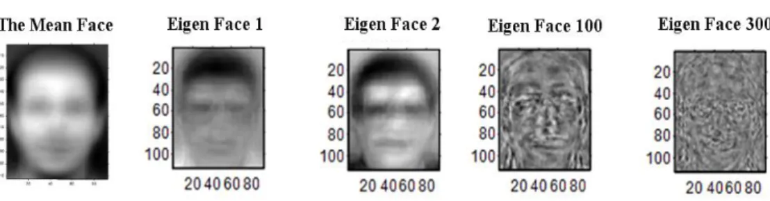
where 𝜇 is the mean of all M images in the training set or the mean face, T is the transpose of its properties and 𝑥𝑖 is the ith image with its columns concatenated in a vector. Figure 2 shows the mean face of the

workand the Eigen faces of the Eigen Faces of the 1st, 2nd, 100th, and the 300th subjects. The Principal components of t eigenvectors are t largest eigenvalues, creating a t dimensional face space [20], [29].

Figure 2. the mean face of the workand the Eigen faces

3.2. Linear Discriminant Analysis (LDA)

Linear Discriminant Analysis (LDA) is used to provide a better classification of data where the data contain high number of classes. This is achieved by finding the best representation among classes. LDA considers for all samples of all classes, the between-class scatter matrix 𝑆𝐵 and the within-class scatter matrix

𝑆𝑊 which are defined by

𝑆

= ∑

𝑀

. (𝑥

− 𝜇). (𝑥

− 𝜇)

(6)

where 𝑀𝑖 is the number of training samples in class i, c is the number of distinct classes, 𝜇𝑖 is the mean

vector of samples belonging to class i and 𝑋𝑖 represents the set of samples belonging toclass i with 𝑥𝑘 being

the k–th image of that class. T is the transpose of its properties. 𝑆𝐵represents the scatter of features around

the overall mean for all face classes and 𝑆𝑊 represents the scatter of features around the mean of each face

class. The goal is to maximize 𝑆𝐵 while minimizing 𝑆𝑤, in other words, maximize the ratio det|𝑆𝐵|/|𝑆𝑤|[29].

This ratio is maximized when the column vectors of the projection matric (𝑊𝐿𝐷𝐴) are the eigenvectors of

𝑆𝑤−1_.𝑆

𝐵. In order to prevent 𝑆𝑤 to become

𝑆𝑊= ∑ ∑𝑥𝑘∈𝑋𝑖(𝑥𝑖− 𝜇𝑖). (𝑥𝑖− 𝜇𝑖)𝑇 𝑐

𝑖=1 (7)

singular, PCA is used as a preprocessing step and the final transformation is 𝑊𝑜𝑝𝑡𝑇 = 𝑊𝐿𝐷𝐴𝑇𝑊𝑃𝐶𝐴𝑇 [20]. 3.3. Kernel Principal Component Analysis (KPCA)

The Kernel projection techniques are used to provide a better discrimination among nonlinearity of data. The main idea is to map input data into a high-dimensional feature space and perform a similar PCA process explained in equation (5). The Kernel methods is used to identify a linear subspace in the high-dimesnional feature space rather than the original input space by avoiding direct computation of the nonlinear mapping Ф through “kernel trick” and derive the kernel transformation matrices based on the kernel matrices of the training data. The rationale of performing such a nonlinear mapping comes from Cover’s theorem which state that “A complex pattern-classification problem cast in a high-dimensional space nonlinearly is more likely to be linearly separable than in a low-dimensional space” [30], [23]. By considering the set of image samples 𝑋𝑘,

𝑥

= [𝑥

, … , 𝑥

]

𝑇

_{∈ 𝑅}

₍₈₎

Kernel PCA is used by projecting each vector x is projected from the input space, 𝑅𝑛, to a high dimensional feature space, 𝑅𝑓_{, by a nonlinear mapping function: Ф: 𝑅}𝑛_{→ 𝑅}𝑓_{, f > n. PCA process is then carried out on}

the kernel subspaces by solving the corresponding eigenvalue problem:

𝜆𝑤Ф_{= 𝐶}Ф_𝑤Ф ₍₉₎

where 𝐶Ф _{is a covariance matrix. All solution 𝑤}Ф _{with 𝜆 ≠ 0 lie in the span of Ф(𝑥}

3.4. Kernel Fisher Analysis (KFA)

KFA is used to reduce the data into a lower subspace and designed to work better than the linear methods where there are complex manifold of data high number of classes. It is performed using the similar procedure of KPCA except that Fisher Linear Discriminant (FLD) is considered instead of PCA after the transformation of the subspace to higher dimension. If 𝑥𝑘 has the same value of equation (8) [31], the same

projection is performed on the vector x. to get the function Ф: 𝑅𝑛_{→ 𝑅}𝑓_{, f > n. Let the projected samples Ф(x)}

be centred in 𝑅𝑓 _{and let the equations that use dot products be formulated for Fisher linear Discrimate}

Analysis (FLD) only. Assume the within-class and between-class scatter matrices be 𝑆𝑊Ф and 𝑆𝐵Ф, to apply

FLD in kernel space, the solution to eigenvalues 𝜆 and eigenvectors 𝑤Ф _of

𝜆𝑆𝑊Ф𝑤Ф = 𝑆𝐵Ф𝑤Ф (10)

are derived by finding the eigenvectors corresponding to largest generalized eigenvalue. The kernel function is introduce defined by

(𝑘𝑟𝑠)𝑡𝑢= k(𝑥𝑡𝑟, 𝑥𝑢𝑠) = Ф(𝑥𝑡𝑟).Ф(𝑥𝑢𝑠`) (11)

where there exists a c-class problem and a r-th sample of class t and the s-th sample of class u be 𝑥𝑡𝑟 and 𝑥𝑢𝑠

respectively (where class t has 𝑙𝑡 samples and class u has 𝑙𝑢 samples). Then finally project Ф(𝑥) to a lower

dimensional space spanned by the eigenvectors 𝑤Ф _{in a way similar to Kernel PCA using Fisherface method}

for face recognition [7],[29].

4. MATCHING

For the matching task, the Mahalinobis Cosine (MAHCOS) distance metric is used. This is because it is the most accurate and efficient in terms of verification, identification and robustness [32]. It measure the cosine of the projected into the recognition space using the corresponding dimensional reduction techniques. After transformations are completed, Mahalinobis Distance measures is used to classify data points by using it to compute the similarity between two faces features. For images u and v with corresponding projections m and n in Mahalinobis space, where m and n are two feature vectors transformed into Mahalinobis space, the Mahalinobis Cosine is [33]:

𝑆𝑀𝑎ℎ𝐶𝑜𝑠𝑖𝑛𝑒(𝑢, 𝑣) = cos (Ɵ𝑚𝑛) =

|𝑚||𝑛|cos (Ɵ𝑚𝑛)

|𝑚||𝑛| = 𝑚.𝑛

|𝑚||𝑛| (12)

with an angle Ɵ defined as the angle between the images after they have been projected into the recognition space as distance between projected images. This distance is refered to as the MahCosine distance.

5. EVALUATION AND RESULTS.

In order to test the performance of each algorithm three different type performance metrics are used with and without the use of Gabor Wavelets. They are the: (a) Cumulative Match Score Curve (CMC), (b) Receiver Operating Characteristic (ROC) Curve, and (C) Expected Performance Curve (EPC). The Cumulative Match Curves (CMCs) is used to calculate the recognition rate. The horizontal axis represents the rank and the vertical axis represents the cumulative match score corresponding to the rank. The lower curve corresponds to the face recognition techniques with a lower performance. The Receiver Operating Characteristic (ROC) curve is a more general curve used in face recognition performance. The horizontal axis represents the false accept rate or FAR, while the vertical axis corresponds to the face verification rate or FVR. The EPC curve shows classifiers from the viewpoint of the tradeoff between false alarm and false rejects probabilities. The EPC curves are produce using an evaluation image set and a test image set which are required. For each 𝛼, the decision threshold that minimizes the weighted sum of the False Acceptance Rate (FAR) and False Rejection Rate (FRR) is computed on the evaluation image set. This threshold is then used on the test images to determine the value of the half total error rates (HTER) defined as HTER = (FAR+FRR)/2. EPC then plot the half total error rate (HTER=0.5(FAR+FRR)) against the parameter 𝛼, which controls the relative importance of the two error rates FAR and FRR in the expression: 𝛼 FAR + (1 −

5.1.

I

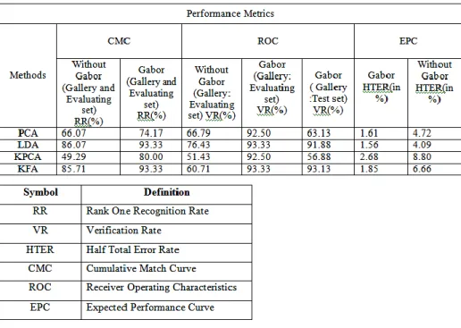
Table 1 gives the detailed summary of the results. There are 400 images containing 10 different images of each person. 120 images are used for training, 160 images are used for testing, the remaining images serve as the evaluation sets. From the results, LDA outperformed other methods in most cases and have a very close recognition rate with KFA. Both LDA and KFA have the highest performance of 93.33 % from the CMC and ROC results when the evaluating set is used with Gabor. Their performance using CMC and ROC with Gabor with more test images is 91.88% and 93.13% respectively (i.e. when the test set is used). It is obvious that the KFA and LDA high performance is due to high number of classes of the images of the system (the database has a total of 40 between-class (matrices) and 10 within-class images). The results of the experiment show that incorporating Gabor image representation makes a notable contribution to the overall face recognition performance of all the algorithms. This is the Gabor wavelets representations are to some extent insensitive to image invariablilities. When more number of test images are used with the Gabor wavelets, there is a general reduction in performance of all the algorithms and there is more reduction when PCA based algorithms are used (PCA and KPCA) than the LDA based algorithms (LDA and KFA). For example with Gabor Wavelets, the ROC performance of both PCA and KPCA recognition rate for the evaluating set(which contain 120 probe images) are both 92.50% and they decrease to 63.13% and 56.88% when the test set (which contains 160 images) is used. With the use of Gabor Wavelets, LDA and KFA ROC performance are both 93.33% when the evaluating set is used and they just decrease to 91.88% and 93.13% when the test set is used. This shows that LDA based algorithms still perform better when the number of test/probe is increased. It can also be seen that KPCA perform worst having the highest error rates (2.68% with Gabor and 8.80% without Gabor). It also has the lowest recognition rate. It performs worse than PCA but only perform better than PCA (from the CMC results with Gabor on the evaluating set) when the Gabor filters is used. Overall the linear based algorithm still performs better than the nonlinear ones.

Table 1. Recognition rates using different Face Recognition performance metrices

The following conclusions are drawn from the results obtained from the experiment (under equal working conditions):

1) The performance of the linear and nonlinear algorithms depends on some conditions. These are explained bellow:

a. The number of classes of a facial recognition system can affects the performance of the type of linear and nonlinear algorithm used. LDA (a linear algorithm) and KFA (a nonlinear algorithm) expressly provides best discrimination among classes.

b. The preprocessing using Gabor filters increases the recognition rate of both the linear and nonlinear algorithms.

c. When more test images are used after preprocessing with Gabor wavelets, there is reduction in recognition rate of all algorithms however the reduction is more for the PCA based algorithms than the LDA based ones. This shows that the increase in number of test images can affects recognition rate (of all the algorithms) negatively but the LDA based (classed based) algorithms are less affected than the PCA based ones.

2) From the overall results the linear algorithms is better than the nonlinear ones.

6. CONCLUSION

The results show that the number of classes and test images of a facial recognition system can have an effect on the recognition rate of a particular algorithm used. Incorporating Gabor image representation with linear and nonlinear algorithms increases their recognition rate. Linear subspace techniques tend to perform better than the nonlinear linear ones from the result of the work carried out. The research will be of outmost importance to any organization that wishes to develop a facial recognition system and know which of the face recognition algorithms have a better recognition rate. This study will also be of immense benefit to prospective researchers who would like to undertake similar studies.

This work is able to compare linear and nonlinear face recognition algorithms produced. The research is only concern about 2D holistic face recognition algorithm. A new development can make use of 2D local based appearance face recognition algorithms using linear and nonlinear algorithms.

REFERENCES

[1] R Sadykhov, I Frolov. The development features of the face recognition system. In IEEE proceedings of the Int. Multiconf. on Comp. Sci. and Infor. Tech. IMCSIT, 2010: 121-128.

[2] W Zhao, R Chellappa, R P J Phillips, A Rosenfeld. Face recognition: A literature survey. ACM Computi. Surv.

2003; 2(4): 399-458.

[3] E. G. Ortiz, BC Becker. Face recognition for web-scale dataset. Comp. Vis. and Image Understanding. 2013; 118: 153-170.

[4] MP Beham, SMM Roomi. Face recognition using appearance based approach: a literature survey. In Proc. IJCA Int. Conference and Workshop on Recent Trends in Technology, TCET, 2012: 16-21.

[5] Huang, W, Yin, H. On nonlinear dimensionality reduction for face recognition. Image and Vision Computing. 2012; 30: 25-366.

[6] J Lu, KN Plataniotis, AN Venetsanopoulos. Face recognition using LDA-based algorithms. IEEE Transactions on Neural Networks. 2003: 14(1): 195–200.

[7] V Struc, F Milhelic, N Pavesic. Combining experts for improved face verification performance. in Proc. IEEE Conf. ERK, 2008: 233-236.

[8] V Balamurugan, M Srinivasan, A Vijayanarayanan, L Bai. A new face recognition techniques using gabor wavelet transform with back propagation neural network. International Journal of Computer Application. 2012: 49(3): 41-46.

[9] A Li, S Shan, W Gao. Coupled Bias–Variance Tradeoff for Cross-Pose Face Recognition. IEEE Transactions on Image Processing. 2012; 21(1): 305,315.

[10] V Struc, N Pavesic. Gabor-based kernel partial-least-squares discrimination features for face recognition.” Institute of Mathematics and Informatics, 2009; 20(1)115-138.

[11] B Zhang, X Chen, S Shan, S, W Gao. Nonlinear face recognition based on maximum average margin criterion.

IEEE Conf. Comput. Vis. Pattern Recog., 2005; 1(4): 554–559.

[12] R Jafri, HR Arabnia. A survey of face recognition techniques. Journal of Information Processing Systems. 2009; 5(2).

[13] R Saha, D Bhattacharjee. Face Recognition Using Eigenfaces” Int. J. Emerging Technology and Adv. Engin., 2013; 3(5): 90-93.

[14] M Nasir (2012, January 25). Getting Ready for Face Recognition - Level 4a tutorial [Online]. Available: http://fewtutorials.bravesites.com

[15] M Turk, A Pentland. Eigenfaces for Recognition. J. Cogn. Neurosc., 1991; 13(1): 71-86.

[16] A Bansal, K Mehta, S Arora, Bansal, A Mehta, K Arora, S. Face Recognition Using PCA and LDA Algorithm," Advanced Computing & Communication Technologies (ACCT), 2012 Second International Conference on , 2012: 251,254, 7-8.

[17] H Yu, H, J Yang. A direct LDA algorithm for high-dimensional data with application to face recognition,” Pattern Recog., 2001; 42: 2067–2070.

[18] MS Bartlett, JR Movellan, TJ Sejnowski. Face recognition by independent component analysis. IEEE Transactions on Neural Networks, 2002; 13(6): 1450-1464.

[19] K Delac, M Grgic, S Grgic. Statistics in face recognition: analyzing probability distributions of PCA, ICA and LDA performance results. Image and Signal Processing and Analysis, 2005. ISPA 2005. Proceedings of the 4th International Symposium on, 2005; 289,294, 15-17.

[20] K Delac, M Grgic, S Grgic. Independent comparative study of PCA, ICA, and LDA on FERET data set. Int. J. of Imaging Systems and Technology, 2006; 15(5): 252-260.

[21] AF Abate, M Nappi, D Ricco, G Sabatino. 2D and 3D face recognition: A survey. Pattern Recognit. 2007; 28: 1886-190.

[22] X He, S Yan, Y Hu, P Niyogi, H Zhang. Face recognition using Laplacianfaces. IEEE Transactions onPattern Analysis and Machine Intelligenc, 2005; 27(3): 328-340.

[23] C Chen, K Xie. Face recognition based on two-dimensional principal component analysis and kernel principal component analysis. Information Technology Journal, Asian Network for Scientific Information IJCSI, 2012; 11(12): 1781-178.

[24] F Igor, S Rauf. The techniques for face recognition with support vector machines. In Proc. of the International Multiconference on Computer Science and Information Technology IMCSIT,2009; 4: 31-36.

[25] MA Kashem, MN AKhter, S Ahmed, AM Alam. Face Recognition System Based on Principal Component Analysis (PCA) with Back Propagation Neural Networks (BPNN). Canadian Journal on Image Processing and Computer Vision, 2011; 2(4): 36-45.

[26] LL Thomas, C Gopakumar, AA Thomas. Face Recognition based on Gabor Wavelet and Backpropagation Neural Networ. J. Sci. and Eng. Research, 2013; 4(6): 2114- 2119.

[27] Shen, L, Bai, L Fairhurst, M. (2006). Gabor wavelets and General Discriminant Analysis for face identification and verification. Image and Vision Computing. Image and Vision Computing, 2007; 25: 553–563.

[28] C. Liu, H Wechsler. Gabor feature based classification using the enhanced fisher linear discriminant model for face recognition, IEEE Transactions on Image Processing, 2002; 11(4): 467-476.

[29] M Yang. Kernel eigenfaces vs. kernel fisherfaces: Face recognition using kernel methods.in Proceedings 5th IEEE Int. Conf. on Automatic Face and Gesture Recog., 2002: 215-220, 21-21.

[30] C Liu. Capitalize on Dimensionality Increasing Techniques for Improving Face Recognition. IEEETransactions on Pattern Analysis and Machine Intelligence, 2006; 28(5): 725-737.

[31] AS Moon, R Srivastava, Y Pandey, (2013). Impact of kernel fisher analysis method on face recognition.

International Journal of Engineering and Advanced Technology, IJEAT, 2013; 2(3).

[32] RM Ibrahim, FEZ Abou-Chadi, AS Samra. Plastic Surgery Face Recognition: A comparative Study of Performance. International Journal of Computer Science IJCSI. 2013; 5(2).

[33] NSS Mar, CB Fookes, PKDV Yarlagadda, (2012). Solder joint defects classification using the Log-Gabor Filter, the Discrete Wavelet Transform and the Discrete Cosine Transform,” In International Conference on Advances in Mechanical and Building, 2012: 9-11.

[34] W Bengio, J Marithoz. The Expected Performance Curve: A New Assessement Measure for Personal Authentication. In Proceedings of Odyssey. The Speaker and Language Recognition Workshop, 2004: 279-284.