ISSN 2307-7743 http://scienceasia.asia
MODELING THE TRANSMISSION OF URINARY TRACT INFECTION (UTI) IN HUMAN POPULATION
XAVERY IDAN MBENA1,∗, DAMIAN KAJUNGURI1,3, JOSEPH SSEBULIBA2
Abstract. Urinary tract infection (UTI) surrounds the urinary tract system and is
main-ly transferred between populations through sex and contact contaminated with UTIs. A
mathematical model is used to examine the transmission of the UTIs. The disease free equilibrium and the basic reproduction number (R0) were established using the next gen-eration matrix method. The basic reproduction number was used to ascertain local and global stabilities for the disease free equilibrium. Sensitive parameters that regulate the
dy-namics of UTI transmission were identified. Numerical simulations were used to verify the analytical solutions of the model. Results show that drying-out stagnant water, disinfection
and sterilization of items in recognition to water and other environment like flows, toilets and bath-houses, may be one of the effective measure for controlling the prevalence and
incidence of UTIs in human population.
1.
IntroductionA urinary tract infection (UTI) is a situation where one or more sections of the urinary system (the kidneys, ureters, urethra, and bladder) is infected. UTIs are the most common of all bacterial infections and can happen at any time in the life of an individual. Approxi-mately 95% of cases of UTIs are caused by bacteria that typically reproduce at the opening of the urethra and move up to the bladder. Often, bacteria spread to the kidney from the bloodstream [24, 22]. It had been known that people were suffering from UTIs before antibiotics were discovered in the early twentieth century; the truth is, nevertheless, there was no real treatment before antibiotics were invented. Doctors recommended a number of tinctures, ointments and special meals/diets to deal with the symptoms, in cases in which the infection spread to the kidneys and bladder and elsewhere, they were honestly helpless. As a last-minute effort, they operated to drain pus from the infected kidneys and hoped the patient would survive. Treatment did not basically change until antibiotics arrived on the scene [21]. The infection customarily begins at the opening of the urethra where the urine goes out of the human body and moves upward into the urinary tract.
UTIs are mostly caused by bacteria and to the small extent by viruses and fungi [8]. The
Key words and phrases. Water and environment, Prevalence, xponentially, UTI transmission, Asymptotically.
c
2017 Science Asia
bacteria usually associated with UTI in hospitals is Uropathogenic Escherichia Coli (UP-EC), signifying more than 80% of infections, the remaining pathogens include Klebsiella species, other coliforms, staphylococci, Enterococcus faecalis and Pseudonzonas aeruginosa [27]. Candida species like Candida albicans are chiefly cause of fungal UTIs specifically in immunosuppressed patients and in those with in-dwelling catheters [10, 18]. Early diagnosis with treatment of UTI is recommended because missed or postponed diagnosis of UTI may cause the failure of appropriate treatment and possibly lead to long-term consequences, in-cluding renal scarring, hypertension, and chronic renal failure [11].
UTI transmission dynamics is complicated by the multiple interactions between the hu-man host, the pathogen and the environment, which contribute to both huhu-man-to-huhu-man and human to environment to human transmission pathways. A deep understanding of the disease transmission dynamics would provide important strategies to the effective preven-tion and control. Mathematical modeling, simulapreven-tion and analysis offer a promising way to look into the nature of UTI dynamics. It is very important to know the life cycles of the pathogens causing UTI. It has been discovered that some pathogens live in human the body and others in aquatic environments. Pathogens like E. coli, klebsiella pneumonia, normally live in human bodies and pathogens like Pseudomonas aeruginosa, Acinetobacter baumannii, Legionella spp., Aeromonas spp., Mycobacterium avium are ubiquitous indige-nous aquatic organisms that can both survive and multiply in water-bath, soil, moist floor, etc. [16]. Furthermore, some pathogens like virus species live in host cells, viruses cannot live by themselves and they need other living cells for reproduction. Viral diseases are quite different from bacterial and fungi diseases, they cannot be treated by antibiotics [25]. The infection to human comes when the healthy person engages with infected human or infested water and other environment.
Signs and symptoms frequently associated with UTIs are a repeated or intense urge to urinate and/or even though little comes out when you do; a burning feeling when you urinate; aching or pressure sores in your back or beneath the abdomen; dark, cloudy, bloody, or abnormal-smelling urine, feeling exhausted, illness [17]. Antibiotic treatment is generally effective for eradication of the infecting strain; however, literature reviews document of increasing antibi-otic resistance, allergic reaction to certain pharmaceuticals, variation on normal gut flora, and failure to avoid recurrent infections represent significant barriers to curative measures.
2.
Model description and formulationThe model system of this study is divided into five major epidemiological classes: Suscepti-ble male Sm, Infected male Im, Susceptible female Sf, Infected female If, Water and other
and female individuals to both sexes are Sm(t) and Sf(t) respectively; male and female
in-dividuals infected with UTI at any time, are Im(t) and If(t) respectively. This means that
N(t) = Sm(t) +Sf(t) +Im(t) +If(t)
Male infection rate from female and female infection rate from male areβf andβm
respective-ly. Susceptible male and female also can get the disease from water and other environment (W e) at any time at the rates βw andβ respectively. The UTI infection rates between male
and female from environment is not the same. Females are more vulnerable than males because of their morphology (i.e. β > βw). The constant per capita recruitment rates into
the susceptible population is Λ and suppose α , φ are per capita natural death rate and, water and other environment dying-out rate respectively. P and 1−Pare the proportion of male and female newborn individuals respectively, and ρ is the Male and female shedding constant rate to water and other environment.
2.1.
Model assumptions(i) Individuals who have frequent and long interactions with infectious individuals and infectious water and other environment experience a high risk of UTI infection.
(ii) Individuals are mixing homogeneously, that is, all susceptible individuals are equally likely to be infected by infectious individuals or infectious water and environment in case of contact.
(iii) Infectious males and females contribute pathogens equally to water and other envi-ronment.
Table 2.1. Model Variables and Parameters
Variables & Parameters Description
N Total population size.
Sm Susceptible male individuals.
Sf Susceptible female individuals.
Im Infectious male individuals.
If Infectious female individuals.
We Infectious W & E.
Λ Per capita birth rate.
P Proportion of male newborn individuals 1−P Proportion of female newborn individuals.
βf Male infection rate from female.
βm Female infection rate from male.
βw Male infection rate from W & E.
β Female infection rate fromW & E.
ρ Male and female shedding rate to W & E.
α Human natural death rate.
φ W & E dying-out rate.
Figure 2.1. Compartmental and Mathematical models for transmission of UTI
The model systems (2.1)-(2.5) satisfies the following initial conditions,
Sm ≥0,Im ≥0,Sf ≥0, If ≥0, andWe≥0.
The total number of human population is given by;
3.
Model System AnalysisFor the disease free equilibrium points (DF E)D∗, we assume there are no pathogens, no infectious individuals and no infectious water and other environment. We resolve the model system (2.1)-(2.5) by setting the infectious compartments to zero, that is Im =If =We = 0
and the results evaluated are as follows
ΛP −(βfSmIf +βwSmWe)−αSm = 0,
(3.1) Sm∗ = ΛP
α .
Λ (1−P)−(βmSfIm+βSfWe)−αSf = 0,
(3.2) Sm∗ = Λ (1−P)
α .
Therefore the disease free equilibrium points are
(3.3) D∗ =
ΛP
α ,0,
Λ (1−P)
α ,0,0
.
3.1.
The basic reproduction number, Ro The basic reproduction number can be usedto analyze the stability of equilibrium points [2]. The basic reproduction number Ro is the
probable number of secondary cases formed by a typical infective individual presented into an entirely susceptible population, without any control measure. The disease-free equilib-rium is said to be locally asymptotically stable if and only if 0 < Ro < 1 and unstable if
Ro >1. A general method for calculating Ro is the next generation method [5]. Using the
method defined by (author?)[30];(author?) [31]. Now
F1(If, We) = (βfSmIf +βwSmWe),F2(Im, We) = (βmSfIm+βSfWe)
and F3(If, If, We) = 0;
V1 =αIm,V2 =αIf and V3 =−ρ(Im+If) +φWe.
Therefore
(3.4) F =
0 βfSm βwSm
βmSm 0 βSf
0 0 0
and
(3.5) V =
α 0 0
0 α 0
−ρ −ρ φ
Hence,
(3.6) F V−1 =
βwΛP ρ α2φ
βfΛP ρ α2 +
betawΛP ρ α2φ
βwΛP αφ βmΛ(1−P)ρ
α2 +
βΛ(1−P)ρ α2φ
βΛ(1−P)ρ α2φ
βΛ(1−P) αφ
0 0 0
.
According to (author?) [4] the largest or dominant eigenvalue obtained is picked as the basic reproduction number Ro.
Then, (3.7)
3.2.
Local stability of disease-free equilibrium point D∗ The local stability of the disease free equilibrium point is examined using trace-determinant or eigenvalues criteria of the Jacobian matrix which is defined as a matrix of all first-order partial derivative of the model system. The equilibrium point is said to be locally asymptotically stable if the Jacobian matrix estimated at that point gives a negative trace and a positive determinant or has negative eigenvalues (author?)[13]. We aim to prove the following Theorem.Theorem 3.1. The disease free equilibrium point (D∗) whenever it occurs is locally asymp-totically stable if Ro <1 and unstable if Ro >1.
Proof
The Jacobian matrix given below is obtained at disease free equilibrium point, (D∗) for model system (2.1) - (2.5)
(3.8) J D∗|(ΛP α ,0,
Λ(1−P)
α ,0,0)
=
−α 0 0 −ΛP βfα −ΛP βw α
0 −α 0 ΛP βf
α
ΛP βw α
0 −Λ(1−αP)βm −α 0 −Λ(1−αP)β
0 Λ(1−αP)βm 0 −α Λ(1−αP)β
0 ρ 0 ρ −φ
.
eliminating the rows and columns the eigenvalues λ1 and λ2 belong.
(3.9) J(D∗)1 =
−α ΛP βfα ΛP βwα
Λ(1−P)βm
α −α
Λ(1−P)β α
ρ ρ −φ
.
With the aid of Maple software, we evaluated and obtained the characteristic polynomial for matrix equation (3.9) as λ3+a1λ2+a2λ+a3 = 0
where
According to Routh-Hurwitz stability criterion the eigenvalues λ1, λ2, λ3, λ4 and λ5 have negative real parts if and only if all coefficients satisfy the following criteria:
H1 =a1 >0,
H2 =a1a2−a3 >0,
H3 =a1a2a3+a1a5−a21a4−a23 >0,
Hence, all roots (eigenvalues) of the characteristic polynomial of our Jacobian matrix have negative real parts [9]. From this we can conclude that the disease free equilibrium point is locally asymptotically stable under these extreme conditions.
3.3.
Global stability of disease-free equilibrium pointD∗ In our model system (2.1) - (2.5), it can be recognized that the disease-free equilibrium point is locally asymptotic stable wheneverRo <1 and unstable whenRo>1. In this section, we have adopted two conditionsthat if agreed, also give the assurance for the global asymptotic stability of the disease-free state [3]. First, the system of differential equations (2.1) - (2.5) must be written in the form:
dX
dt =F (X, I),
(3.10)
dI
dt =G(X, I) ; G(X,0) = 0,
(3.11)
where X ∈ Rr, I ∈ Rn, r, n,≥ 0, and G(X,0) = 0. The components of X indicate the
represent the number of infected population liable to transmitting the UTI. D∗ = (X∗,0), denotes the disease-free equilibrium point of this system. The fixed point D∗ = (X∗,0) is a globally asymptotically stable equilibrium point for this system provided that Ro < 1 (i.e.
locally asymptotically stable) and the following two conditions are satisfied:
where the Jacobian Q =
∂G ∂I
(X∗,0) is an M-matrix (the off diagonal elements of Q are
non negative) and Ω is the invariant region. For this case the disease free equilibrium point is now signified as D∗ = (X∗,0), X∗ =ΛP
α ,0, Λ(1−P)
α ,0,0
. If the model system (2.1) - (2.5)
fulfills the conditions (H1) and (H2), then conferring to(author?)[3] the following theorem holds.
Theorem 3.2. The equilibrium point D∗ = (X∗,0) of the model system (2.1) - (2.5) is globally asymptotically stable if Ro ≤1 and the conditions (H1) and (H2) are met.
Proof
We initiate our proof by outlining X = (Sm, Sf) and I = (Im, If, We). We look on the two
vector valued functions F(X, I) and G(X, I). We adopt the method done by (author?)
[14]. By considering the equation dXdt =F(X,0), from condition (H1), we obtain
(3.12)
( dSm
dt = ΛP −αSm, dSf
dt = Λ (1−P)−αSf.
X∗ = ΛαP,(Λ(1−αP)) is globally asymptotically stable equilibrium point for the reduced
system model equations dX
dt =F(X,0).
We then computeG(X, I) =
∂G ∂I
(X∗,0)I−Gˆ(X, I) and show that ˆG(X, I)≥0;
∂G ∂I
(X∗,0) =
−α ΛP βfα ΛP βwα
Λ(1−P)βm
α −α
Λ(1−P)β α
ρ ρ −φ
, (3.13)
this is an M-matrix with non-negatives off diagonal elements. Then,
∂G ∂I
(X∗,0)I =
−αIm+βfβf ΛP βf
α +βwWe ΛP βw
α
βmIm
Λ(1−P)βm
α +−αIf +βWe
Λ(1−P)β α
ρIm+ρIf +−φWe
Hence,
ˆ
G(X, I) =
∂G ∂I
(X∗,0)I−G(X, I),
ˆ
G(X, I) = 0 0 0 . (3.15)
Therefore, ˆG(X, I)≥0. In this case the Theorem 3.2 has been proved and we can conclude that the disease free equilibrium point is globally asymptotically stable under these extreme circumstances.
3.4.
The existence of endemic equilibrium point E∗ The state where the disease cannot be completely eliminated but remains in the population is called the endemic equi-librium state.Furthermore, the endemic equiequi-librium point is said to be locally stable whenRo > 1 and unstable when 0< Ro < 1 [28]. For the disease to continue in the population,
the susceptible classes and the Infectious classes must not be zero at equilibrium state [14]. In other words, the endemic equilibrium state is given as
E∗ = Sm∗, Im∗, Sf∗, If∗, We∗6= (0,0,0,0,0),
with the fact that Sm∗ >0, Im∗ >0, Sf∗ >0, If∗ >0 andWe >0.
Initially, we evaluated the variables We∗ and Sm∗ from model system (2.1) - (2.5) respectively as follows
We∗ = ρ I ∗ m+I
∗ f
φ ,
(3.16)
Im∗ = αI ∗
f αφ+βρI ∗ f
−Λ (1−P) βρIf∗
Λ (1−P) (βmφ+βρ)−αIf∗(βmφ+βρ)
,
(3.17)
If∗ = αI ∗
m(αφ+βwρIm∗)−ΛP (βwρIm∗)
ΛP(βfφ+βwρ)−αIm∗ (βfφ+βwρ)
.
(3.18)
For the positivity, existence and uniqueness of endemic equilibrium point, the following conditions in above equations must hold,
αIf∗ αφ+βρIf∗>Λ (1−P) βρIf∗, Λ (1−P) (βmφ+βρ)> αIf∗(βmφ+βρ),
αIm∗ (αφ+βwρIm∗)>ΛP(βwρIm∗), and ΛP (βfφ+βwρ)> αIm∗ (βfφ+βwρ).
Furthermore, we can produce polynomials for Im∗ and If∗ by substitution of If∗ into Im∗ and vice versa respectively [33]. We obtain the following polynomial equations
Im∗ and If∗ are solutions of the above equations with coefficients of A1, A2, A3, A4, B1, B2, B3, and B4.
(3.20)
It follows that, Im∗ , If∗ = 0, and
A1Im∗3+A2Im∗2+A3Im∗ +A4, B1If∗3+B2If∗2+B3If∗+B4 = 0. (3.21)
For the endemic equilibrium point to exist, the solutions of (3.21) must be real and positive. Also, since Im∗ , If∗ = 0, the viral free steady state is said to be in neutral state (i.e. exists an infection or no infection) [23]. From these conditions, we conclude that the endemic equilibrium solution is stable when Ro >1, and it exhibits persistence of UTI transmission
in the population.
4.
Numerical Results, Simulation and DiscussionBasic model simulations are important aspects in Mathematical modeling. We understand the behaviour of UTI dynamics when an endemic situation persists and demonstrate how susceptible sub-populations interact with infected sub-populations. We identified the effects of the most positive and negative sensitive parameters with respect to basic reproduction number (Ro). The simulation of the model system of the equations has been plot to examine
the dynamic forces of UTI in the entire population when there is no intervention.
4.1.
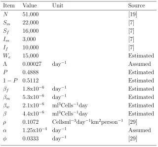
Parameter estimation The total population of consideration is an area sparingly populated with a density of 51 persons per square kilometre with deviation across the regions in Tanzania [19]. We estimate the proportion of male and female newborn individuals, taking into consideration that the life expectancy at birth of the male and female newborn individuals in Tanzania [15] are 63.5% (out of all male newborns) and 66.4% (out of all female newborns) respectively which are equivalent to P = 0.4888 and 1−P = 0.5112.(author?) [6] revealed that the cumulative incidence rate of UTI was three times greater in girls (females) by 6.6% than boys (males) by 1.8%. In this study we estimated the male infection rate from female, βf as 0.0000018 and the female infection rate from male, βm
Table 4.1. Model Variables and Parameters and their description
Item Value Unit Source
N 51,000 [19]
Sm 22,000 [7]
Sf 16,000 [7]
Im 3,000 [7]
If 10,000 [7]
We 15,000 Estimated
Λ 0.00027 day−1 Assumed
P 0.4888 Estimated
1−P 0.5112 Estimated
βf 1.8x10⁻⁶ day−1 Estimated
βm 5.3x10⁻⁶ day−1 Estimated
βw 2.1x10⁻⁶ ml3Cells−1day Estimated
β 4.4x10⁻⁶ ml3Cells−1day Estimated
ρ 0.1072 Cellsml−3day−1km2person−1 [29]
α 1.25x10⁻⁴ day−1 Assumed
φ 0.0333 day−1 [29]
4.2.
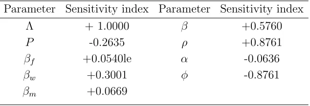
Sensitivity analysis of Ro Sensitivity analysis expresses how significant eachpa-rameter is in disease transmission. Sensitivity analysis plays a central role in epidemiological modeling. With the help of Maple 18 software we noticed that reproduction number for disease free equilibrium (DFE), Ro is 0.208 while for endemic equilibrium (EE),Ro is 3463.
In this paper we adopt the method of determining the sensitivity analysis as used by [26, 20]. The basic reproduction numberRoof UTI depends on nine parameters, we deduce an
analyt-ical expression for its sensitivity to every parameter using the normalized forward sensitivity indices of Ro with respect to parameterspj involved in Ro as shown below:
(4.1) ΥRopj = ∂R0
∂pj
× pj
R0
.
For instance, the sensitivity indices of Ro with respect to Λ is calculated as
(4.2) ΥRoΛ = ∂R0
∂Λ ×
pj
R0 = 1.
Other differentials produces long expressions, to determine the sensitivity index of the re-spective parameter we substitute the parameter values specified in Table 4.1. Following the same technique we can obtain the sensitivity indices for ΥRoβm, ΥRoβ
f, Υ Ro βw, Υ
Ro
β , ΥRoα , Υ Ro φ ,
ΥRo
ρ and Υ Ro
P as tabulated in the Table 4.2. The dynamics of these sensitivity analysis done
Table 4.2. Model Variables and Parameters
Parameter Sensitivity index Parameter Sensitivity index
Λ + 1.0000 β +0.5760
P -0.2635 ρ +0.8761
βf +0.0540le α -0.0636
βw +0.3001 φ -0.8761
βm +0.0669
positive parameter is the Per capita birth rate (Λ). The following parameters in their pos-itive descending order of sensitivity are: male and female shedding rate to water and other environment (ρ), male infection rate from water and other environment (βw), female
infec-tion rate from water and other environment (β), female infection rate from male (βm), male
infection rate from female (βf) and human mortality/death rate (α). The positive sign of
the stated parameters indicates that decreasing (increasing) one of these parameters while keeping other parameters constant drops (rises) the value of the basic reproduction number. Taking an example for the sensitivity indices ofRo with respect toβ is 0.5760, this indicates
that increasing female infection rate from water and other environment by 50%, increases the value of basic reproduction number by 57% and hence increases the existence of the UTI and vice versa. Conversely, water and other environment dying-out rate (φ) is the most negative parameter. Other parameters with negative sensitivity indices are human mortality/death rate (α) and proportion of male newborn individuals (P). This implies that increasing (de-creasing) this parameter while keeping the other parameters constant decreases (increases) the value of basic reproduction number Ro and hence decreases (increases) the persistence
of UTI.
Table 4.3. Population under consideration
Item Population in square kilometres Population of Sombetini
Susceptible male 22 22,000
Infected male 3 3,000
Susceptible female 16 16,000
Infected female 10 10,000
Water and other environment 15 15,000
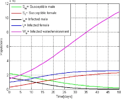
Figure 4.1. Characteristics of five model system variables
Figures 4.1 shows the dynamics in humans and, water and other environment populations, displaying the characteristics of five state variables Sm, Im, Sf, If and We with given time
and finally reach the endemic equilibrium point. The sub-populations of infected male and infected female caused by UTI infections rise exponentially to a certain point in time then decline to reach endemic equilibrium point as they undergo a natural death. The decrease in susceptible male and female sub-populations lead into the growth of the insignificantly infected male and female that raise exponentially after sometime they start diminishing be-cause of natural death and as they gain more infection from infected male and female and infected water and other environment to join the severely infected male and female class then finally reach endemic equilibrium point. The severely infected male and female ad-vance exponentially to a certain point in time then start deteriorating due to natural death and lastly achieves endemic equilibrium point. The population of pathogens in water and other environment increases exponentially with time to a certain point and then declines to reach endemic equilibrium point as they die naturally. They die-out when the water and other environment is dried-up and as they burrow into the earth. The lines of susceptible male and female sub-populations decrease and extend approaching to zero asymptotically meaning that some susceptible male and female sub-populations will not all get infection or die naturally.
Another important aspect in epidemiology is the area which concerned with the existence of disease in populations. Public health professionals and epidemiologists use each measure of disease frequency for particular purposes. Prevalence and Incidence are greatest useful for valuing the effectiveness of plans that try to stop disease from occurring in the entire population [1]. Researchers who investigate the sources of disease prefer to examine new cases (incidence) over prevailing ones (prevalence) since they are usually concerned in expo-sures that advance to emerging the disease. Prevalence it combines incidence and survival to obscures underlying relationships.
In figures 4.2 and 4.3 we present the numerical outcomes with respect to the negatively sensitive parameter to Ro, which is φ (dying-out rate of pathogens in water and other
water and other environment dying-out rate decreases and vice versa.
Figure 4.2. Disease prevalence with respect to variation of water and other
environment dying-out rate.
In figure 4.3, we noticed that disease incidence to the human sub-populations on the increase or decrease of water and other environment dying-out rate, φ. From the figure we deduced that when the pathogens dying-out rate is very big or small, the incidence increases sharply for male and female sub-populations within the first 15 and 12 days respectively, then drops exponentially approaching zero asymptotically. The incidence drops sharply for male and female sub-populations within the first 3 and 1 days respectively.
Figure 4.3. Disease incidence with respect to variation of water and other
environment dying-out rate.
and/or treating water and other environment on UTI prevalence and incidence as one way of eradicating the infections in the human population.
5.
ConclusionIn this paper one major issue that surrounds UTIs modeling is conferred. We found that the infectious water and other environment is the reservoir and habitats for bacteria and other UTI pathogens and is a major source of UTIs transmission route. Increased awareness of water and other environment as a possible major source of UTIs transmission route is need-ed [12]. We are not intending to marginalize other transmission paths, awareness should be taken even to them.
We recommend the following for reduction and prevention on the prevalence and incidence of UTIs in human population: Applying a rational approach to disinfection and sterilization of items in recognition to water and other environment like floors, toilets and bathhouses. Others are drying out unnecessary standing water, treating water bodies (reservoir) like swimming pools and sewages regularly with recommended antibiotics. Domestic animals are among carriers of UTI pathogens, precautions on health care should be taken in consider-ation when providing services. Also avoid staying with wet clothes for long time especially to children and practicing sex to a man/woman who you dont know their health status. Education campaign and implementing prevailing infection control strategies to the entire population is necessary. Attend hospital treatments when you notice the UTI symptoms, this can help to reduce the intensity of infections.
References
[1] A. Aschengrau, G. R. Seage, et al., Essentials of epidemiology in public health, Jones & Bartlett Publishers, 2013.
[2] Castillo-Chavez, Mathematical approaches for emerging and reemerging infectious diseases: models, methods, and theory, Springer, 2002.
[3] C. Castillo-Chavez, Z. Feng, and W. Huang, On the computation of r0 and its
role on global stability, 2002, Math. la. asu. edu/chavez/2002/JB276. pdf, (2002). [4] O. Diekmann, The construction of next-generation matrices for compartmental
epi-demic models, Journal of the Royal Society Interface, (2009), p. rsif20090386.
[5] O. Diekmann, J. A. P. Heesterbeek, and J. A. Metz, On the definition and
the computation of the basic reproduction ratio r0 in models for infectious diseases in heterogeneous populations, Journal of mathematical biology, 28 (1990), pp. 365–382. [6] B. Foxman, Epidemiology of urinary tract infections: incidence, morbidity, and
[7] , Urinary tract infection syndromes: occurrence, recurrence, bacteriology, risk fac-tors, and disease burden, Infectious disease clinics of North America, 28 (2014), pp. 1–13. [8] B. Foxman and P. Brown, Epidemiology of urinary tract infections: transmission
and risk factors, incidence, and costs, Infectious disease clinics of North America, 17 (2003), pp. 227–241.
[9] A. A. Gebremeskel and H. E. Krogstad, Mathematical modelling of endemic
malaria transmission, American Journal of Applied Mathematics, 3 (2015), pp. 36–46.
[10] M. Grabe, R. Bartoletti, T. Bjerklund Johansen, T. Cai, M. C¸ ek,
B. K¨oves, K. Naber, R. Pickard, P. Tenke, F. Wagenlehner, et al.,
Guide-lines on urological infections. european association of urology (eau), 2015.
[11] S. Hansson and U. Jodal, Dimercapto-succinic acid scintigraphy instead of voiding
cystourethrography for infants with urinary tract infection, The Journal of urology, 172 (2004), pp. 1071–1074.
[12] D. Johnson, L. Lineweaver, and L. M. Maze, Patients bath basins as potential
sources of infection: a multicenter sampling study, American Journal of Critical Care, 18 (2009), pp. 31–40.
[13] J. Kahuru, L. Luboobi, and Y. Nkansah-Gyekye, Stability analysis of the
dy-namics of tungiasis transmission in endemic areas, Asian Journal of Mathematics and Applications, 2017 (2017).
[14] T. Kinene, L. S. Luboobi, B. Nannyonga, and G. G. Mwanga,A mathematical
model for the dynamics and cost effectiveness of the current controls of cassava brown streak disease in uganda, Journal of Mathematical and Computational Science, 5 (2015), p. 567.
[15] H. Masanja, D. de Savigny, P. Smithson, J. Schellenberg, T. John, C.
M-buya, G. Upunda, T. Boerma, C. Victora, T. Smith, et al., Child survival
gains in tanzania: analysis of data from demographic and health surveys, The Lancet, 371 (2008), pp. 1276–1283.
[16] M. Middelboe, Bacterial growth rate and marine virus–host dynamics, Microbial E-cology, 40 (2000), pp. 114–124.
[17] S. J. Midthun, Criteria for urinary tract infection in the elderly: variables that
chal-lenge nursing assessment, Urologic Nursing, 24 (2004), p. 157.
[18] D. Minardi, G. dAnzeo, D. Cantoro, A. Conti, and G. Muzzonigro,Urinary
tract infections in women: etiology and treatment options, Int J Gen Med, 4 (2011), pp. 333–343.
[19] T. NBS, Population and housing census: population distribution by administrative
ar-eas, Ministry of Finance, Dar es Salaam, (2012).
[20] R. C. Ngeleja, L. S. Luboobi, and Y. Nkansah-Gyekye, Modelling the
[21] J. C. Nickel,Management of urinary tract infections: historical perspective and cur-rent strategies: part 2modern management, The Journal of urology, 173 (2005), pp. 27– 32.
[22] L. E. Nicolle, Catheter-related urinary tract infection, Drugs & aging, 22 (2005),
pp. 627–639.
[23] M. J. Ongala Jacob Otieno and O. Paul, Mathematical model for
pneumoni-a dynpneumoni-amics with cpneumoni-arriers, International Journal of Mathematical Analysis, 7 (2013), pp. 2457–2473.
[24] P. C. Pappas,Laboratory in the diagnosis and management of urinary tract infections, Medical Clinics of North America, 75 (1991), pp. 313–325.
[25] S. A. Rahman, Study of Infectious Diseases by Mathematical Models: Predictions and
Controls, PhD thesis, The University of Western Ontario, 2016.
[26] H. S. Rodrigues, M. T. T. Monteiro, and D. F. Torres, Sensitivity analysis
in a dengue epidemiological model, in Conference Papers in Science, vol. 2013, Hindawi Publishing Corporation, 2013.
[27] S. M. Soto, Importance of biofilms in urinary tract infections: new therapeutic
ap-proaches, Advances in Biology, 2014 (2014).
[28] A. Ssematimba, J. Mugisha, and L. S. Luboobi,Mathematical models for the dy-namics of tuberculosis in density-dependent populations: The case of internally displaced peoples camps (idpcs) in uganda, (2005).
[29] J. H. Tien and D. J. Earn,Multiple transmission pathways and disease dynamics in a
waterborne pathogen model, Bulletin of mathematical biology, 72 (2010), pp. 1506–1533. [30] P. Van Den Driessche, Some epidemiological models with delays, tech. report, 1994.
[31] P. Van den Driessche and J. Watmough,Reproduction numbers and sub-threshold
endemic equilibria for compartmental models of disease transmission, Mathematical bio-sciences, 180 (2002), pp. 29–48.
[32] U. Water, Gender, water and sanitation: A policy brief, UN, New York, (2006).
[33] J. Zhang, J. Jia, and X. Song, Analysis of an seir epidemic model with saturated incidence and saturated treatment function, The Scientific World Journal, 2014 (2014).
1
Department of Applied Mathematics and Computational Science, Nelson Mandela African
Institution of Science and Technology, P.O. Box 447 Arusha, Tanzania
2
Department of Mathematics, Makerere University, P.O. Box 7062 Kampala, Uganda
3
Department of Mathematics, Kabale University, P.O. Box 317 Kabale, Uganda