Weiguo Ma, Xia Xu and Hairong Zhu
College of Electrical Engineering, Nantong University, Nantong, ChinaNetworked Non-fragile H∞ Control
for Lipschitz Nonlinear System with
Quantization and Packet Dropout in
Both Feedback and Forward Channels
The networked non-fragile H∞ control problem for Lipschitz nonlinear system with quantization and packet dropout in both feedback and forward channels is investigated in this paper. The sensor measurement and controller output are quantized by logarithmic quantizers before beeing transmitted over the net
-work. The packet transmissions in the communication channels from the sensor to the controller and from the controller to the actuator are modeled as Markov chains respectively. Based on the Lyapunov functional approach, the networked non-fragile H∞ controller is designed to stabilize the Lipschitz nonlinear system and achieve the prescribed H∞ performance. Finally, a numerical example is provided to illustrate the effec
-tiveness and superiority of the proposed method. ACM CCS (2012) Classification: Applied computing → Operations research → Industry and manufactur -ing → Command and control
Information systems → Information systems applica
-tions → Process control systems
Keywords: non-fragile H∞ control, Lipschitz nonlin
-ear system, quantization, packet dropout
1. Introduction
Networked control system where the control loop is closed through communication network has attracted considerable attention in recent
years. Networked control system has been ap
-plied in a broad range of areas such as compli
-cated industrial control system, remote control of robot, unmanned aircrafts and vehicles, etc
[1]. In networked control system, the sensors, controllers and actuators exchange information
via the shared communication network. The in
-troduction of network in control loop gives rise to some issues such as data quantization [2],
[3], network induced delay [4] and packet drop
-out [5] – [8], which complicate the analysis and design of networked control systems.
There exists perturbation in the coefficient of
the controller due to the effect of finite resolu
-tion measuring instruments, finite word length
and roundoff errors [9]. Therefore, it is neces
-sary that the non-fragile controller is designed. Many efforts have been made in networked control system recently. The network induced delay is transformed into the uncertainties of the system coefficients for networked control system with network induced delay. Then non-fragile controllers are designed based on robust
control theory [10] – [12]. In [13], the net
-worked control system is modeled as time de
-lay system, and then the non-fragile guaranteed cost fault tolerant controller is designed. Using
the structure vertex separator method, the prob
-lem of non-fragile H∞ control is studied for networked continuous time linear system with time delay and logarithmic quantizer in [14].
Considering the randomly occurring gain vari
-ations, distributed delays and channel fadings,
system, Liu and Sun design the non-fragile con
-troller based on parallel distributed compensa
-tion and multiple Lyapunov func-tions method [17]. It is worth pointing out that the existing literature is concerned with non-fragile control of networked control system with quantization and/or network induced delay. To the best of the authors' knowledge, the problem of networked non-fragile H∞ control for Lipschitz nonlinear
system subject to quantization and packet drop
-out, both in the feedback and forward paths, has not been fully investigated, which motivates the present study.
The rest of this paper is organized as follows. In Section 2, the effects of quantization and packet dropout are analyzed. The networked control
system is modeled as a Markovian jumping sys
-tem. The sufficient condition for the existence of non-fragile H∞ controller is given in terms
of linear matrix inequality in Section 3. A sim
-ulation example is presented to illustrate the ef
-fectiveness of the proposed method in Section 4. In Section 5, conclusions are given.
Notation: Rn denotes the n dimensional Euclid
-ean space. || || stands for the Euclid-ean norm.
I and 0 denote the identity and zero matrices
of compatible dimensions respectively. Pr[·]
means the occurrence probability of event ''·''.
E{x} stands for the expectation of stochastic
variable x. MT and M –1 denote respectively
the transpose and inverse of a matrix M. X > 0
(X < 0) means that the matrix X is real sym
-metric positive definite (negative definite). The asterisk ''*'' in a matrix is used to represent the
term that is induced by symmetry. diag{M1,...,
M2} stands for a block-diagonal matrix with the
matrices M1,...,M2 on the diagonal.
2. Problem Formulation and
Preliminaries
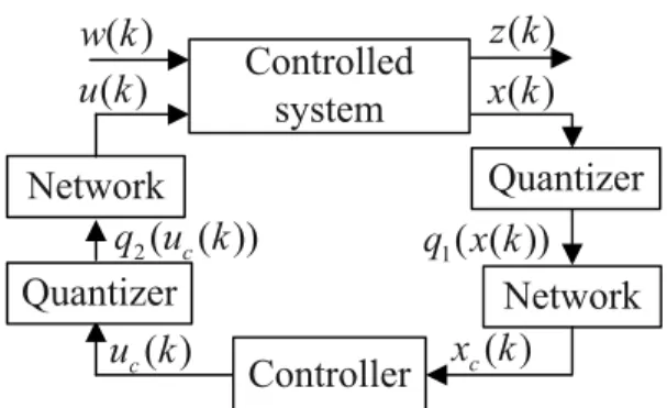
The diagram of networked control for Lipschitz nonlinear system studied in this paper is shown in Figure 1. Lipschitz nonlinear system is very common. For example, the sinusoidal terms encountered in some problems of robotics are
global Lipschitz. Considered in a given neigh
-borhood, most nonlinearities are local Lipschitz [18].
The controlled system is described by
1 2
( 1) ( ) ( ) ( )
( , ( ))
( ) ( ) ( )
x k Ax k B u k B w k Ff k x k
z k Cx k Dw k
+ = + +
+
= +
(1)
where x(k) ∈ Rn is the state, u(k) ∈ Rp is the
control input, w(k) ∈Rm is the disturbance be
-longing to L2 [0,∞], z(k) ∈Rq is the controlled
output. A, B1, B2, F, C and D are known con
-stant matrices with appropriate dimensions.
f (k,x (k)) is a nonlinear vector function that is
assumed to be Lipschitz with respect to x(k),
i.e. there exists known constant matrix F1 such
that f(0,0) = 0, || f(k,x1 (k)) – f(k,x2 (k))|| ≤ ||F1 (x1 (k) – x2 (k))||.
The system state is quantized before beeing transmitted to the controller via the network due
to the limited bandwidth. Logarithmic quantiz
-ers are essential for quadratic stabilization via quantized feedback if a coarse quantization density is required. Nonlogarithmic quantizers such as finite quantizers and linear quantizers are unsuitable [19]. The following logarithmic quantizer is used in this paper
1
1
, if / (1 )
/(1 ) , 0
( )
0, if 0
( ), if 0
i i i
u u v
u v
q v
v
q v v
δ δ
+ < ≤
− >
= =
− − <
(2)
where the set of quantized levels U = {±ui, ui =
ρiu0, i = ±1, ±2,...} ∪ {±u0} ∪ {0}, 0 < ρ < 1,
u0 > 0, δ = (1 – ρ)/(1 + ρ), ρ is the quantization
density of q1 (ν). The quantized state can be de
-scribed by
When the guided system is controlled, the con
-troller uc(k) = V ‒ (Kα(k) + ∆K)xc(k), where V is
the reference signal.
The output of the controller uc(k) is also quan
-tized by a logarithmic quantizer q2 (ν) which is
similar to the state quantizer q1 (ν). The control
input of the system is described by
2
( ) ( )( ( )) ( )
(1 ( )) ( 1)
c
u k k I H k u k k u k
β β
= +
+ − − (8)
where ||H2 (k)|| ≤ δ2, δ2 = (1 – ρ2)/(1 + ρ2), ρ2 is
the quantization density of q2 (ν).
Defining the augmented state x(k) = [xT(k),
xcT(k ‒ 1), uT(k ‒ 1)]T, the networked control
system can be modeled as
( 1) ( ( ), ( )) ( ) ( )
( , ( ))
( ) ( ) ( )
x k A k k x k Bw k Ff k x k
z k Cx k Dw k
α β
+ = +
+
= +
(9)
where
11 12 13
21 22
31 32 33
( ( ), ( )) 0 ,
A A A
A k k A A
A A A
α β
=
2
, , [ ,0,0], ,
0 0
0 0
B F
B F C C D D
= = = =
11 1 2 ( )
1
( ) ( ) ( ( ))(
)( ( )),
k
A A k k B I H k K
K I H k
α
β α
∆
= + +
+ +
12 ( )(1 ( )) (1 2( ))( ( )k ),
A =β k −α k B I H k K+ α +∆K
13 1(1 ( )), 21 ( )( 1( )),
A =B −β k A =α k I H k+
22 (1 ( )) ,
A = −α k I
31 2 ( )
1
( ) ( )( ( ))( )
( ( )),
k
A k k I H k K
I H k
α
β α ∆Κ
= + +
⋅ +
32 ( )(1 ( ))( 2( ))( ( )k ),
A =β k −α k I H k K+ α +∆K
33 (1 ( )) .
A = −β k I
Because the networked control system is mod
-eled as Markovian jumping system, we intro
-duce the following stochastically stable and H∞ performance definitions and a lemma which will be used in the sequel.
[
]
1 1 1 1
1
( ( )) ( ( )) ( ( ))
( ( )) ( )
T n
q x k q x k q x k I H k x k
= = +
(3)
where ||H1 (k)|| ≤ δ1.
When the quantized data are transmitted over
the network, it is supposed that the network in
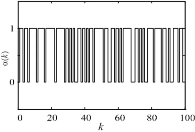
-duced delay is small enough to be neglected. In addition, due to the disturbance or network congestion, the data packet may be dropped out, which is common in wireless network. The packet transmission process can be modeled as Markov chain [8]. Assume that Markov chains
α(k) and β(k) denote the packet transmission
process in the channels from the sensor to the
controller and from the controller to the actu
-ator respectively. The finite state sets are Φ1 =
{0,1} and Φ2 = {0,1}. The state 0 means that the
data packet is dropped out. The state 1 indicates that the data packet is transmitted successfully. The transition probability matrices of Markov chains are P = [λij] and Q = [πrs] with
[
]
Pr ( 1) | ( )
ij k j k i
λ = α + = α = , λij ≥ 0,
1
0 ij 1 j= λ =
∑
, πrs =Pr ([
β k+ =1) s| ( )β k =r]
,πrs ≥ 0,
∑
1s=0πrs =1, ∀i, j ∈Φ1, ∀r, s ∈Φ2.The input of the controller can be described by
1
( ) ( )( ( )) ( )
(1 ( )) ( 1)
c
c
x k k I H k x k k x k
α α
= +
+ − − (4) It is necessary that the controller which is part
of a closed-loop system can tolerate some un
-certainty in its coefficients [9]. Consider the non-fragile controller
u kc( ) (= Kα( )k +∆K x k) ( )c (5)
where Kα(k) is the controller gain, ∆K stands for the controller gain perturbations which are of additive and multiplicative forms:
∆ =K M F k N2 2( ) ,2 F k F k2T( ) ( )2 ≤I (6) ∆ =K M F k N K3 3( ) 3 α( )k , F k F k3T( ) ( )3 ≤I (7) where M2, N2, M3, N3 are known constant ma
-trices.
Controlled system
Quantizer
Network Controller
Network
( )
z k
( )
w k
( )
x k
( )
u k
1( ( )) q x k
( )
c
u k x kc( )
Quantizer2
( ( ))c q u k
system, Liu and Sun design the non-fragile con
-troller based on parallel distributed compensa
-tion and multiple Lyapunov func-tions method [17]. It is worth pointing out that the existing literature is concerned with non-fragile control of networked control system with quantization and/or network induced delay. To the best of the authors' knowledge, the problem of networked non-fragile H∞ control for Lipschitz nonlinear
system subject to quantization and packet drop
-out, both in the feedback and forward paths, has not been fully investigated, which motivates the present study.
The rest of this paper is organized as follows. In Section 2, the effects of quantization and packet dropout are analyzed. The networked control
system is modeled as a Markovian jumping sys
-tem. The sufficient condition for the existence of non-fragile H∞ controller is given in terms
of linear matrix inequality in Section 3. A sim
-ulation example is presented to illustrate the ef
-fectiveness of the proposed method in Section 4. In Section 5, conclusions are given.
Notation: Rn denotes the n dimensional Euclid
-ean space. || || stands for the Euclid-ean norm.
I and 0 denote the identity and zero matrices
of compatible dimensions respectively. Pr[·]
means the occurrence probability of event ''·''.
E{x} stands for the expectation of stochastic
variable x. MT and M –1 denote respectively
the transpose and inverse of a matrix M. X > 0
(X < 0) means that the matrix X is real sym
-metric positive definite (negative definite). The asterisk ''*'' in a matrix is used to represent the
term that is induced by symmetry. diag{M1,...,
M2} stands for a block-diagonal matrix with the
matrices M1,...,M2 on the diagonal.
2. Problem Formulation and
Preliminaries
The diagram of networked control for Lipschitz nonlinear system studied in this paper is shown in Figure 1. Lipschitz nonlinear system is very common. For example, the sinusoidal terms encountered in some problems of robotics are
global Lipschitz. Considered in a given neigh
-borhood, most nonlinearities are local Lipschitz [18].
The controlled system is described by
1 2
( 1) ( ) ( ) ( )
( , ( ))
( ) ( ) ( )
x k Ax k B u k B w k Ff k x k
z k Cx k Dw k
+ = + +
+
= +
(1)
where x(k) ∈ Rn is the state, u(k) ∈ Rp is the
control input, w(k) ∈Rm is the disturbance be
-longing to L2 [0,∞], z(k) ∈Rq is the controlled
output. A, B1, B2, F, C and D are known con
-stant matrices with appropriate dimensions.
f (k,x (k)) is a nonlinear vector function that is
assumed to be Lipschitz with respect to x(k),
i.e. there exists known constant matrix F1 such
that f(0,0) = 0, || f(k,x1 (k)) – f(k,x2 (k))|| ≤ ||F1 (x1 (k) – x2 (k))||.
The system state is quantized before beeing transmitted to the controller via the network due
to the limited bandwidth. Logarithmic quantiz
-ers are essential for quadratic stabilization via quantized feedback if a coarse quantization density is required. Nonlogarithmic quantizers such as finite quantizers and linear quantizers are unsuitable [19]. The following logarithmic quantizer is used in this paper
1
1
, if / (1 )
/(1 ) , 0
( )
0, if 0
( ), if 0
i i i
u u v
u v
q v
v
q v v
δ δ
+ < ≤
− >
= =
− − <
(2)
where the set of quantized levels U = {±ui, ui =
ρiu0, i = ±1, ±2,...} ∪ {±u0} ∪ {0}, 0 < ρ < 1,
u0 > 0, δ = (1 – ρ)/(1 + ρ), ρ is the quantization
density of q1 (ν). The quantized state can be de
-scribed by
When the guided system is controlled, the con
-troller uc(k) = V ‒ (Kα(k) + ∆K)xc(k), where V is
the reference signal.
The output of the controller uc(k) is also quan
-tized by a logarithmic quantizer q2 (ν) which is
similar to the state quantizer q1 (ν). The control
input of the system is described by
2
( ) ( )( ( )) ( )
(1 ( )) ( 1)
c
u k k I H k u k k u k
β β
= +
+ − − (8)
where ||H2 (k)|| ≤ δ2, δ2 = (1 – ρ2)/(1 + ρ2), ρ2 is
the quantization density of q2 (ν).
Defining the augmented state x(k) = [xT(k),
xcT(k ‒ 1), uT(k ‒ 1)]T, the networked control
system can be modeled as
( 1) ( ( ), ( )) ( ) ( )
( , ( ))
( ) ( ) ( )
x k A k k x k Bw k Ff k x k
z k Cx k Dw k
α β
+ = +
+
= +
(9)
where
11 12 13
21 22
31 32 33
( ( ), ( )) 0 ,
A A A
A k k A A
A A A
α β
=
2
, , [ ,0,0], ,
0 0
0 0
B F
B F C C D D
= = = =
11 1 2 ( )
1
( ) ( ) ( ( ))(
)( ( )),
k
A A k k B I H k K
K I H k
α
β α
∆
= + +
+ +
12 ( )(1 ( )) (1 2( ))( ( )k ),
A =β k −α k B I H k K+ α +∆K
13 1(1 ( )), 21 ( )( 1( )),
A =B −β k A =α k I H k+
22 (1 ( )) ,
A = −α k I
31 2 ( )
1
( ) ( )( ( ))( )
( ( )),
k
A k k I H k K
I H k
α
β α ∆Κ
= + +
⋅ +
32 ( )(1 ( ))( 2( ))( ( )k ),
A =β k −α k I H k K+ α +∆K
33 (1 ( )) .
A = −β k I
Because the networked control system is mod
-eled as Markovian jumping system, we intro
-duce the following stochastically stable and H∞ performance definitions and a lemma which will be used in the sequel.
[
]
1 1 1 1
1
( ( )) ( ( )) ( ( ))
( ( )) ( )
T n
q x k q x k q x k I H k x k
= = +
(3)
where ||H1 (k)|| ≤ δ1.
When the quantized data are transmitted over
the network, it is supposed that the network in
-duced delay is small enough to be neglected. In addition, due to the disturbance or network congestion, the data packet may be dropped out, which is common in wireless network. The packet transmission process can be modeled as Markov chain [8]. Assume that Markov chains
α(k) and β(k) denote the packet transmission
process in the channels from the sensor to the
controller and from the controller to the actu
-ator respectively. The finite state sets are Φ1 =
{0,1} and Φ2 = {0,1}. The state 0 means that the
data packet is dropped out. The state 1 indicates that the data packet is transmitted successfully. The transition probability matrices of Markov chains are P = [λij] and Q = [πrs] with
[
]
Pr ( 1) | ( )
ij k j k i
λ = α + = α = , λij ≥ 0,
1
0 ij 1 j= λ =
∑
, πrs =Pr ([
β k+ =1) s| ( )β k =r]
,πrs ≥ 0,
∑
1s=0πrs =1, ∀i, j ∈Φ1, ∀r, s ∈Φ2.The input of the controller can be described by
1
( ) ( )( ( )) ( )
(1 ( )) ( 1)
c
c
x k k I H k x k k x k
α α
= +
+ − − (4) It is necessary that the controller which is part
of a closed-loop system can tolerate some un
-certainty in its coefficients [9]. Consider the non-fragile controller
u kc( ) (= Kα( )k +∆K x k) ( )c (5)
where Kα(k) is the controller gain, ∆K stands for the controller gain perturbations which are of additive and multiplicative forms:
∆ =K M F k N2 2( ) ,2 F k F k2T( ) ( )2 ≤I (6) ∆ =K M F k N K3 3( ) 3 α( )k , F k F k3T( ) ( )3 ≤I (7) where M2, N2, M3, N3 are known constant ma
-trices.
Controlled system
Quantizer
Network Controller
Network
( )
z k
( )
w k
( )
x k
( )
u k
1( ( )) q x k
( )
c
u k x kc( )
Quantizer2
( ( ))c q u k
Definition 1 [20]. When w(k) = 0, the net
-worked control system (9) is said to be stochas
-tically stable if for every initial state (x(0),α(0),
β(0)), Ε
{
k∞0 x k( ) 2}
= < ∞
∑
.Definition 2 [20]. Given a scalar γ > 0 , the net
-worked control system (9) is said to have an H∞
performance γ, if
{
}
2{
}
0 T( ) ( ) 0 T( ) ( )
k Ε z k z k γ k Ε w k w k
∞ ∞
= < =
∑
∑
for all nonzero w (k) ∈ L2 [0,∞〉 under zero ini -tial condition.
Lemma 1 [21]. Given matrices Γ1 = Γ1T, Γ2 and
Γ3of appropriate dimensions, then Γ1 + Γ2F4(k)
Γ3 + Γ3T F4T (k) Γ2 < 0 holds for all F4(k) satis -fying F4T (k)F
4(k) ≤ I, if and only if there exists
scalar ε > 0 such that Γ1 + ε‒1Γ2Γ2T + ε Γ3T Γ3 < 0.
3. Non-Fragile H∞ Controller Design
In this section, we explore the sufficient condi
-tion of the existence of non-fragile H∞ control
-ler for networked control system (9). First, we establish the sufficient condition of stability for the networked control system.
Theorem 1. Given the quantization densi
-ties ρ1, ρ2 and controller gain Kα(k) + ∆K, the networked control system (9) is stochastically
stable if there exist symmetric positive defi
-nite matrices P(i,r) = diag{P1 (i,r), P2 (i,r),
P3 (i,r)}, i ∈Φ1, r ∈Φ2, scalar ε > 0 such that the following matrix inequalities hold
31 32 33
( , ) * *
0 * 0
P i r
I
εΦ ε
Ξ Ξ Ξ
− +
− <
(10)
where
31 ( , ), ( , ), ( , ), ( , ) ,
T
T T T T
A i r A i r A i r A i r
Ξ =
32 , , , ,
T T T T T
F F F F
Ξ =
{
}
133 0 0
1 1
0 1 1 0
1 1 1
1/ ( ) (0,0),
1/ ( ) (0,1), 1/ ( ) (1,0),
1/ ( ) (1,1) ,
i r
i r i r i r
diag P
P P
P
Ξ λ π
λ π λ π
λ π − − − − = − − − −
1 1 0 .
0 0
T
F F
Φ =
Proof. Consider the following Lyapunov func -tional V[x(k),α(k) = i, β(k) = r] = xT(k)P(i,r)x(k) where P(i,r) = diag{P1 (i,r), P2 (i,r), P3 (i,r)}, P1 (i,r), P2 (i,r) and P3 (i,r) are symmetric positive definite matrices.
As f T (k,x (k)) f (k,x (k)) ≤ xT(k)F
1T F1x (k), there
exists ε > 0 so that εxT(k)F
1T F1x(k) ‒ f T(k,x(k)) f(k,x(k)) ≥ 0.
Taking the difference of V[x(k),α(k) = i, β(k) =
r] along the trajectory of system (9) with w(k)
= 0, we can obtain
{
}
( ) [ ( 1), ( 1), ( 1) | ( ),
( ) , ( ) ] [ ( ), ( ) ,
( ) ] T( ) ( , ) ( )
V k V x k k k x k
k i k r V x k k i
k r k i r k
∆ Ε α β
α β α
β ζ Ξ ζ
= + + + = = − = = = where 11 ( , ) *
( , )i r Ti r T ,
F HA HF I
Ξ Ξ Φ ε = −
( )k x k f k x kT( ), T( , ( )) ,T
ζ =
11
( , )i r A i r HA i r P i rT( , ) ( , ) ( , ) ,
Ξ = − +εΦ
1 1
0 0 ij rs ( , ). j s
H =
∑ ∑
= = λ π P j sThus,
( ) T( ) ( ) T( ) ( )
V k k k x k x k
∆ ≤ −φζ ζ ≤ −φ
where ϕ is the least eigenvalue of −Ξ( , )i r . Then,
{
2}
10 ( ) T(0) ( (0), (0)) (0)
k x k x P x
Ε ∞ φ− α β
= < < ∞
∑
Therefore, by Definition 1, the networked con
-trol system (9) is stochastically stable. The proof is completed.
The following theorem proposes the sufficient condition for the existence of non-fragile H∞ controller for networked control system (9). Theorem 2. Given a scalar γ > 0, quantiza
-tion densities ρ1 and ρ2, the networked control
system (9) is stochastically stable and has an
H∞ performance γ, if there exist scalars ε1 >
0, ε2 > 0, ε3 > 0, ε4 > 0, ε5 > 0, ε6 > 0, sym
-metric positive definite matrices X(i,r) = diag
{X1 (i,r), X2 (i,r), X3 (i,r)}, i ∈Φ1, r ∈ Φ2, Q,
matrices Y0 and Y1 such that the following lin
-ear matrix inequalities hold
1,11 1,21 1,22 1,31 1,33 1,41 1,44 * * * * * 0 0 * 0 0 Ω Ω Ω Ω Ω Ω Ω
<
(11) 2,11 2,21 2,22 2,31 2,33
2,41 2,42 2,44
2,51 2,52 2,54 2,55
* * * *
* * *
0 * * 0
0 *
0 Ω
Ω Ω
Ω Ω
Ω Ω Ω
Ω Ω Ω Ω
<
(12) 3,11 3,21 3,22 3,31 3,33
3,41 3,42 3,44
* * * * * 0 0 * 0 Ω Ω Ω Ω Ω
Ω Ω Ω
<
(13) 4,11 4,21 4,22
4,31 4,32 4,33
4,41 4,42 4,43 4,44
4,51 4,52 4,53 4,54 4,55
* * * *
* * *
* * 0
* Ω
Ω Ω
Ω Ω Ω
Ω Ω Ω Ω
Ω Ω Ω Ω Ω
<
( 14)
where Ω1,11 = diag{‒X(0,0), ‒γ2I, ‒ε
1I},
1 1 1,21 1 1 (0,0) (0,0) (0,0) (0,0) (0,0) (0,0) (0,0) (0,0)
A X B F
A X B F
A X B F
A X B F
ε ε Ω ε ε =
Ω1,22 = diag{‒1/(λ00π00)X(0,0), ‒1/(λ00π01)X(0,1), ‒1/(λ01π00)X(1,0), ‒1/(λ01π01)X(1,1)}, Ω1,31 =
[C,D,0], Ω1,33 = ‒I, Ω1,41 = [F1,X(0,0),0,0], F1
= [F1, 0, 0], Ω1,44 = ‒ε1I, Ω2,11 = diag{‒X(0,1), ‒γ2I, ‒ε
1I},
2,21 1 2,21 1 2,21 2,21 1 2,21 1 , B F B F B F B F Π ε Π ε Ω Π ε Π ε =
1 1 0
2,21 2
0
(0,1) 0
0 (0,1) 0 ,
0 0
AX B Y
X Y Π =
Ω2,22 = diag{‒1/(λ00π10)X(0,0), ‒1/(λ00π11)X(0,1),
‒1/(λ01π10)X(1,0), ‒1/(λ01π11)X(1,1)},
1
2,31
1 1
(0,1) 0 0 0
(0,1) 0 0 0 0
CX D
F X
Ω =
{
}
2,33 diag I, 1I ,
Ω = − −ε
2,41
2 2
0 0 0 0 0
,
0 N X (0,1) 0 0 0
Ω =
2,42 2,42 2,42 2,42 2,42 ,
Ω = Π Π Π Π
2 2 1 2 2
2,42 0 ,
0 0 0
T T T
M B M
ε ε
Π =
{
}
2,44 diag 2I, 2I ,
Ω = −ε −ε
2,51
0
0 0 0 0 0 ,
0 Y 0 0 0
Ω =
2,52 2,52, 2,52, 2,52, 2,52 ,
Ω = Π Π Π Π
3 1 3
2,52 0 ,
0 0 0
T
B I
ε ε
Π =
2,54 2 2 0 0 , 0 M Ω ε =
{
2}
2,55 diag 3I, 3 2I ,
Ω = −ε −ε δ
{
2}
3,11 diag X(1,0), I, 1I ,
Ω = − −γ −ε
1 1 3
3,21 1
3
(1,0) 0 (1,0)
(1,0) 0 0 ,
0 0 (1,0)
AX B X
X
X
Π
=
Ω3,22 = diag{‒1/(λ10π00)X(0,0), ‒1/(λ10π01)X(0,1), ‒1/(λ11π00)X(1,0), ‒1/(λ11π01)X(1,1)},
1
3,31
1 1
(1,0) 0 0 0
, (1,0) 0 0 0 0
CX D
F X
Ω =
3,33 2,33,
Ω =Ω
3,41
1
0 0 0 0 0
, (1,0) 0 0 0 0
X
Ω =
3,42 3,42, 3,42, 3,42, 3,42 ,
Ω = Π Π Π Π
4
3,42 00 0 0I 0 ,
ε
Π =
{
2}
3,44 diag 4I, 4 1I ,
Ω = −ε −ε δ
{
}
{
}
2
4,11 1
2
1
(1,1), ,
,0,0 ,
diag X I I
diag Q
Ω γ ε
δ
= − − −
+
4,21 1
4,21 1 4,21
4,21 1
4,21 1
,
B F B F B F B F
Π ε
Π ε
Ω
Π ε
Π ε
=
1 1 1
4,21 1
1
(1,1) 0 0
(1,1) 0 0 ,
0 0
AX B Y
X Y
Π
+
=
Ω4,22 = diag{‒1/(λ10π10)X(0,0), ‒1/(λ10π11)X(0,1), ‒1/(λ11π10)X(1,0), ‒1/(λ11π11)X(1,1)},
1
4,31 1 1
(1,1) 0 0 0
(1,1) 0 0 0 0 ,
0 0 0 0 0
CX D
F X
Ω
=
4,32 4,32, 4,32, 4,32, 4,32 ,
Ω = Π Π Π Π
4,32
1 1 1
0 0 0
0 0 0 ,
T T T
Y B I Y
Π
=
{
}
4,33 diag I, I Q, ,
Ω = − −ε −
4,41
2 1
0 0 0 0 0
, (1,1) 0 0 0 0
N X
Ω =
4,42 4,42, 4,42, 4,42, 4,42 ,
Ω = Π Π Π Π
5 2 1 5 2
4,42 0 ,
0 0 0
T T T
M B M
ε ε
Π =
4,43
2 1
0 0 0
,
0 0 N X (1,1)
Ω =
{
}
4,44 diag 5I, 5I ,
Ω = −ε −ε
4,51
1
0 0 0 0 0 , 0 0 0 0
Y
Ω =
4,52 4,52, 4,52, 4,52, 4,52 ,
Ω = Π Π Π Π
6 1 6
4,52 0 ,
0 0 0
T
B I
ε ε
Π =
4,53 4,54
5 2
1
0 0
0 0 0
, ,
0
0 0 Y M
Ω Ω
ε
= =
{
2}
4,55 diag 6I, 6 2I .
Ω = −ε −ε δ
Furthermore, the additive non-fragile H∞ con
-troller gains in the form of (5) and (6) are K0 =
Y0 X2‒1(0,1) and K1 = Y1 X1‒1(1,1).
Proof. Consider the following Lyapunov func -tional V[x(k),α(k) = i, β(k) = r] = xT(k)P(i,r)x(k) where P(i,r) = diag{P1 (i,r), P2 (i,r), P3 (i,r)}, P1 (i,r), P2 (i,r) and P3 (i,r) are symmetric
positive definite matrices.
Taking the difference of V [x(k),α (k) = i, β (k)
= r] along the trajectory of system (9), we can
obtain
{
}
1
( ) [ ( 1), ( 1), ( 1) | ( ),
( ) , ( ) ] [ ( ), ( ) ,
( ) ] T( ) ( , ) ( )
V k V x k k k x k
k i k r V x k k i
k r k i r k
∆ Ε α β
α β α
β η Θ η
= + + +
= = − =
= =
where η( )k = x k w k f k x kT( ), T( ), T( , ( )) ,T
1,11
1 1,22
( , ) * *
( , ) ( , ) ( , ) * ,
( , )
T
T T T
i r
i r B HA i r i r
F HA i r F HB F HF I
Θ
Θ Θ
ε
=
−
1,11( , )i r A i r HA i r P i rT( , ) ( , ) ( , ) ,
Θ = − +εΦ
1 1
0 0 ij rs ( , ), j s
H =
∑ ∑
= = λ π P j s1,22( , )i r B HBT .
Θ =
Consider the following performance index
{
2}
0 ( ) ( ) ( ) ( ) .
N T T
N k
J =Ε
∑
= z k z k −γ w k w k Under zero initial condition, we can obtain
{
}
{
}
2 0
0
2 0
[ ( ) ( ) ( ) ( )
( )] ( )
( ) ( , ) ( )
N T T
N k
N k N T
k
J z k z k w k w k
V k V k
k i r k
Ε γ
∆ Ε ∆
η Θ η
=
=
=
= −
+ −
<
∑
∑
∑
where
[
]
2 1
2
( , ) ( , ) , ,0 , ,0
0, ,0 0, ,0 .
T T
i r i r C D C D
I I
Θ Θ
γ
= +
−
Case 1. i = 0, r = 0. Let X1 (i,r) = P1‒1(i,r), X2
(i,r) = P2‒1(i,r), X3 (i,r) = P3‒1(i,r), ε1 = ε‒1,
both sides of (11) are respectively multiplied by diag{Λ1,11,Λ1,22,Λ1,33,Λ1,44}, where Λ1,11 =
diag{P(0,0),I,εI}, Λ1,22 = diag{I,I,I,I}, Λ1,33
= I, Λ1,44 = I. By Schur complement, one can
obtain Θ2 (0,0) < 0.
Case 2. i = 0, r = 1. Let Y0 = K0X2 (0,1), both sides of (12) are respectively multiplied by
diag{Λ2,11,Λ2,22,Λ2,33,Λ2,44 Λ2,55}, where Λ2,11 =
diag{P(0,1),I,εI}, Λ2,22 = diag{I,I,I,I}, Λ2,33 = diag{I,I}, Λ2,44 = Λ2,33, Λ2,55 = Λ2,33. Using Lemma 1 and the method similar to case 1, one can obtain Θ2 (0,1) < 0.
Case 3. i = 1, r = 0. By the method similar to
Case 2, one can obtain Θ2 (1,0) < 0.
Case 4.i = 1, r = 1. Let Q = ε4P1‒1(1,1), P1‒1(1,1),
Y1 = K1P1‒1(1,1), by the method similar to Case
2, one can obtain Θ2 (1,1) < 0.
According to the above, Θ2 (i,r) < 0 implies that matrix inequalities (10) hold. So the networked
control system (9) is stochastically stable. On
the other hand, as N → ∞,
{
2}
0 T( ) ( ) T( ) ( ) 0.
k
J Ε ∞ z k z k γ w k w k
∞ =
∑
= − <Therefore, from definition 2 it follows that the
networked control system (9) has an H∞ perfor
-mance γ. This completes the proof.
Remark 1. The sufficient condition for the ex
-istence of multiplicative non-fragile H∞ con
-troller in the form of (5) and (7) is similar to
(11), (12), (13) and (14), except that M2 and N2
are substituted by M3 and N3Kα(k) respectively. Remark 2. As the packet transmissions in both feedback and forward channels are considered simultaneously, the controller can be designed by the proposed algorithm. The obtained result is general.
Remark 3. The networked control system is modeled by augmented state, so the dimension of the system is enlarged, which makes the computation complex.
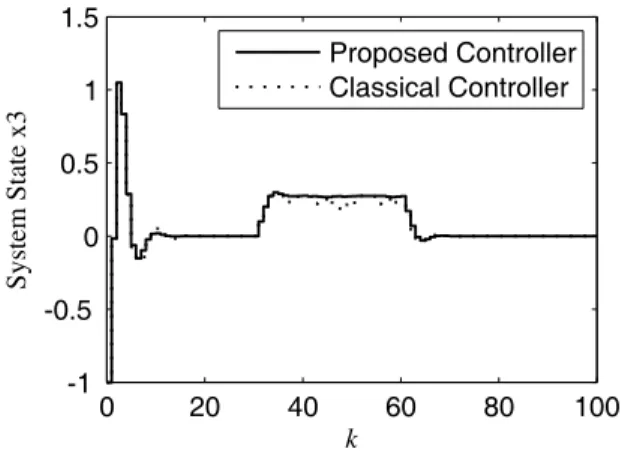
4. Numerical Example
To illustrate the effectiveness of the method proposed in this paper, consider the Lipschitz nonlinear system with the following parameters [6]
1 2
0.75 0.5 0 1 0.2
0.7 0 0 , 0 , 0.2 ,
0 1 0 0 0.2
A B B
−
= = =
1
2
3 0.03sin( ( )) 1 0 0
0.01sin( ( ))
0 1 0 , ( , ( )) ,
0 0 1 0.02sin( ( ))
x k x k
F f k x k
x k
= =
[
]
0,0 30
( ) 0.8,30 60, 0.1,0,0 , 0.6.
0, 60
k
w k k C D
k
≤ <
= ≤ < = =
≥
The additive controller gain perturbations are
M2 = 0.1 and N2 = [0.1,0.1,0.2], while the quan
-tization densities of the quantizer of the system
state and controller output are respectively ρ1
= 0.5 and ρ2 = 0.6. The transition probability
1 1 3
3,21 1
3
(1,0) 0 (1,0)
(1,0) 0 0 ,
0 0 (1,0)
AX B X
X
X
Π
=
Ω3,22 = diag{‒1/(λ10π00)X(0,0), ‒1/(λ10π01)X(0,1), ‒1/(λ11π00)X(1,0), ‒1/(λ11π01)X(1,1)},
1
3,31
1 1
(1,0) 0 0 0
, (1,0) 0 0 0 0
CX D
F X
Ω =
3,33 2,33,
Ω =Ω
3,41
1
0 0 0 0 0
, (1,0) 0 0 0 0
X
Ω =
3,42 3,42, 3,42, 3,42, 3,42 ,
Ω = Π Π Π Π
4
3,42 00 0 0I 0 ,
ε
Π =
{
2}
3,44 diag 4I, 4 1I ,
Ω = −ε −ε δ
{
}
{
}
2
4,11 1
2
1
(1,1), ,
,0,0 ,
diag X I I
diag Q
Ω γ ε
δ
= − − −
+
4,21 1
4,21 1 4,21
4,21 1
4,21 1
,
B F B F B F B F
Π ε
Π ε
Ω
Π ε
Π ε
=
1 1 1
4,21 1
1
(1,1) 0 0
(1,1) 0 0 ,
0 0
AX B Y
X Y
Π
+
=
Ω4,22 = diag{‒1/(λ10π10)X(0,0), ‒1/(λ10π11)X(0,1), ‒1/(λ11π10)X(1,0), ‒1/(λ11π11)X(1,1)},
1
4,31 1 1
(1,1) 0 0 0
(1,1) 0 0 0 0 ,
0 0 0 0 0
CX D
F X
Ω
=
4,32 4,32, 4,32, 4,32, 4,32 ,
Ω = Π Π Π Π
4,32
1 1 1
0 0 0
0 0 0 ,
T T T
Y B I Y
Π
=
{
}
4,33 diag I, I Q, ,
Ω = − −ε −
4,41
2 1
0 0 0 0 0
, (1,1) 0 0 0 0
N X
Ω =
4,42 4,42, 4,42, 4,42, 4,42 ,
Ω = Π Π Π Π
5 2 1 5 2
4,42 0 ,
0 0 0
T T T
M B M
ε ε
Π =
4,43
2 1
0 0 0
,
0 0 N X (1,1)
Ω =
{
}
4,44 diag 5I, 5I ,
Ω = −ε −ε
4,51
1
0 0 0 0 0 , 0 0 0 0
Y
Ω =
4,52 4,52, 4,52, 4,52, 4,52 ,
Ω = Π Π Π Π
6 1 6
4,52 0 ,
0 0 0
T
B I
ε ε
Π =
4,53 4,54
5 2
1
0 0
0 0 0
, ,
0
0 0 Y M
Ω Ω
ε
= =
{
2}
4,55 diag 6I, 6 2I .
Ω = −ε −ε δ
Furthermore, the additive non-fragile H∞ con
-troller gains in the form of (5) and (6) are K0 =
Y0 X2‒1(0,1) and K1 = Y1 X1‒1(1,1).
Proof. Consider the following Lyapunov func -tional V[x(k),α(k) = i, β(k) = r] = xT(k)P(i,r)x(k) where P(i,r) = diag{P1 (i,r), P2 (i,r), P3 (i,r)}, P1 (i,r), P2 (i,r) and P3 (i,r) are symmetric
positive definite matrices.
Taking the difference of V [x(k),α (k) = i, β (k)
= r] along the trajectory of system (9), we can
obtain
{
}
1
( ) [ ( 1), ( 1), ( 1) | ( ),
( ) , ( ) ] [ ( ), ( ) ,
( ) ] T( ) ( , ) ( )
V k V x k k k x k
k i k r V x k k i
k r k i r k
∆ Ε α β
α β α
β η Θ η
= + + +
= = − =
= =
where η( )k = x k w k f k x kT( ), T( ), T( , ( )) ,T
1,11
1 1,22
( , ) * *
( , ) ( , ) ( , ) * ,
( , )
T
T T T
i r
i r B HA i r i r
F HA i r F HB F HF I
Θ
Θ Θ
ε
=
−
1,11( , )i r A i r HA i r P i rT( , ) ( , ) ( , ) ,
Θ = − +εΦ
1 1
0 0 ij rs ( , ), j s
H =
∑ ∑
= = λ π P j s1,22( , )i r B HBT .
Θ =
Consider the following performance index
{
2}
0 ( ) ( ) ( ) ( ) .
N T T
N k
J =Ε
∑
= z k z k −γ w k w k Under zero initial condition, we can obtain
{
}
{
}
2 0
0
2 0
[ ( ) ( ) ( ) ( )
( )] ( )
( ) ( , ) ( )
N T T
N k
N k N T
k
J z k z k w k w k
V k V k
k i r k
Ε γ
∆ Ε ∆
η Θ η
=
=
=
= −
+ −
<
∑
∑
∑
where
[
]
2 1
2
( , ) ( , ) , ,0 , ,0
0, ,0 0, ,0 .
T T
i r i r C D C D
I I
Θ Θ
γ
= +
−
Case 1. i = 0, r = 0. Let X1 (i,r) = P1‒1(i,r), X2
(i,r) = P2‒1(i,r), X3 (i,r) = P3‒1(i,r), ε1 = ε‒1,
both sides of (11) are respectively multiplied by diag{Λ1,11,Λ1,22,Λ1,33,Λ1,44}, where Λ1,11 =
diag{P(0,0),I,εI}, Λ1,22 = diag{I,I,I,I}, Λ1,33
= I, Λ1,44 = I. By Schur complement, one can
obtain Θ2 (0,0) < 0.
Case 2. i = 0, r = 1. Let Y0 = K0X2 (0,1), both sides of (12) are respectively multiplied by
diag{Λ2,11,Λ2,22,Λ2,33,Λ2,44 Λ2,55}, where Λ2,11 =
diag{P(0,1),I,εI}, Λ2,22 = diag{I,I,I,I}, Λ2,33 = diag{I,I}, Λ2,44 = Λ2,33, Λ2,55 = Λ2,33. Using Lemma 1 and the method similar to case 1, one can obtain Θ2 (0,1) < 0.
Case 3. i = 1, r = 0. By the method similar to
Case 2, one can obtain Θ2 (1,0) < 0.
Case 4.i = 1, r = 1. Let Q = ε4P1‒1(1,1), P1‒1(1,1),
Y1 = K1P1‒1(1,1), by the method similar to Case
2, one can obtain Θ2 (1,1) < 0.
According to the above, Θ2 (i,r) < 0 implies that matrix inequalities (10) hold. So the networked
control system (9) is stochastically stable. On
the other hand, as N → ∞,
{
2}
0 T( ) ( ) T( ) ( ) 0.
k
J Ε ∞ z k z k γ w k w k
∞ =
∑
= − <Therefore, from definition 2 it follows that the
networked control system (9) has an H∞ perfor
-mance γ. This completes the proof.
Remark 1. The sufficient condition for the ex
-istence of multiplicative non-fragile H∞ con
-troller in the form of (5) and (7) is similar to
(11), (12), (13) and (14), except that M2 and N2
are substituted by M3 and N3Kα(k) respectively. Remark 2. As the packet transmissions in both feedback and forward channels are considered simultaneously, the controller can be designed by the proposed algorithm. The obtained result is general.
Remark 3. The networked control system is modeled by augmented state, so the dimension of the system is enlarged, which makes the computation complex.
4. Numerical Example
To illustrate the effectiveness of the method proposed in this paper, consider the Lipschitz nonlinear system with the following parameters [6]
1 2
0.75 0.5 0 1 0.2
0.7 0 0 , 0 , 0.2 ,
0 1 0 0 0.2
A B B
−
= = =
1
2
3 0.03sin( ( )) 1 0 0
0.01sin( ( ))
0 1 0 , ( , ( )) ,
0 0 1 0.02sin( ( ))
x k x k
F f k x k
x k
= =
[
]
0,0 30
( ) 0.8,30 60, 0.1,0,0 , 0.6.
0, 60
k
w k k C D
k
≤ <
= ≤ < = =
≥
The additive controller gain perturbations are
M2 = 0.1 and N2 = [0.1,0.1,0.2], while the quan
-tization densities of the quantizer of the system
state and controller output are respectively ρ1
= 0.5 and ρ2 = 0.6. The transition probability