Distributed Multi-ant Algorithm for Capacity Vehicle Route Problem
Jie Li, Yi Chai and Cao Yuan Chongqing University
E-mail: [email protected], [email protected], [email protected]
Keywords:capacity vehicle route problem, distributed multi-ant algorithm, cellular ants, performance potential
Received:November 2, 2010
This paper proposes a Distributed Multi-ant Algorithm for capacity vehicle route problem (CVRP) where cooperation is helpful for accelerating prior solution by executing a decomposition-based separation methodology for the unsteady capacity constraints. It decreases the complex coupling network with others to solve small instances with less correlation in parallel processing. The main goal of this work is to play well on large scale CVRP with interaction between subsystems and certain state vectors. The results show that Distributed Multi-ant Algorithm plays better performance on average solution and the importance of potential action is analyzed.
Povzetek: Za problem CVRP je razvit izboljšan postopek, temeljeˇc na algoritmih z mravljami.
1
Introduction
With decomposition, every subsystem could be described as a Markov Decision Process (MDP) model: Let M =
{S, A, T, R, f v} be a five tuple model, whereS = {s} is a set of states, A = {a} is a set of actions, T =
{p(·|s, a), s∈S, a∈A}is the next-state transition prob-ability distribution, withp(· | s, a)describing the proba-bility of actionain statestos,. R(s, a, s,)is the reward
function. f v is the additional reward function. π(s)is a policy function in the state space. The discussion about ap-plicability and feasibility is based on discount value MDP and Q-learning.
Algorithms works on CVRP are researched for years. Edge assembly (EAX) crossover with well-known local searches is employed to CVRP (Yuichi Nagata et al, 2009). De-oxyribonucleic acid (DNA) computing model and a modi-fied Adleman-Lipton model accelerate the search on large nodes CVRP (Yeh Chung Wei, 2009). Ellipse rule ap-proach reduces the average distance to the lower bound by about 44% (Santos Luis et al, 2009). A multi-objective evolutionary algorithm is used for CVRP (Borgulya Istvan, 2008). Particle swarm optimization (PSO) can also apply for CVRP, in two models (Ai The Jin et al, 2009). Cel-lular GAs has solved vehicle routing problem, minimized transportation cost and recombined a new problem (Carlos Bermudez et al, 2010) and genetic algorithm has worked at it fewer than 100 nodes (Wang Chungho et al, 2010). Normally, it is solved based on decentralized model. How-ever, coupling among subsystems (called SCVRP in the pa-per) is not considered well and being trap into a local solu-tion or no solusolu-tion easily, deviating from what we expected. Multi-ant algorithm is extension of ant algorithm who plays a better performance in the best solution and used to VRP already (Yuvraj Gajpal et al, 2009). The ant isn’t punished
if the strategy misleads it to suboptimal policies. And if there isn’t new knowledge during states, the reward func-tion is still working accumulafunc-tion. In this paper, decom-position of CVRP based on a distributed model is pre-sented with iteration and cooperation between subsystems searching for their own optimization by distributed multi-ant algorithm. As cooperation, a cellular multi-ant contacts with other ants both in its own subsystem and others through reward strategies obtained whenever the related strategy is optimal by traditional relative reinforcement learning. Re-ward shaping undergoes through structuring additional re-ward function for distributed multi-ant algorithm, making it more efficient.
As the large scale of CVRP is divided into smaller SCVRPs in a distributed system where bunches of cellular ants set to seek an optimal solution of corresponding subgraph for SCVRP. On the one hand, cellular ants in the same sub-system collaborate with each other and refresh their own knowledge. On the other hand, cellular ants in different SCVRP regenerate strategies as they meet in the crossed arcs over several disparate SCVRPs.
2
Decomposition algorithms for
CVRP
For the limited capacity constraint, a large scale of CVRP is decomposed into SCVRPs with unsteady capacity con-straints in the distributed system. The mathematical model of CVRP is transformed throughT ree Description(Chen Yulin et al, 2002). An algorithm named Tree Cut-Set (TCS) is proposed for decomposition. The number of subsystems is determined by the carrying capability of vehicles, de-mands of customers and connection between customers.
A large scale of undirected graph can be transformed into complete trees and split into subgraphs where leaves of subgraphs are the compound boundaries. Then, the seman-tic representation of CVRP could be replaced by SCVRPs. Based on these definitions in (Y Xiang, 1996), calculation must comply for some principle as follows:
(1) a∗b=ab
(2) (a∗b),=ab,+a,b=a+b
(3) aΛb=a,b+ab,=a+b
(4) (aΛb),= (ab),= 1
In ripping, two subgraphs are brought out and the sum-mation of their semantic representation is equat to the orig-inal graph. We can call the origorig-inal graph the father graph of the two subgraphs. It requires the knowledge of the in-terface between SCVRPs only, not the knowledge of the internal structure of them. TCS is applied to closed the structural details to separate the model. In the result, ev-ery SCVRP could obtain its own solution through an in-dependent set of ants and the link between them is loosely coupled by employing TCS. Whatever the structure CVRP is, TCS is suitable for it, whether customers may join and leave or not.
We will explain the theory oft−sepsetcouple based on d−sepset(Li Yan et al, 2004).
Definition 1 In a tree, for tree-nodei, there is only two parents and one child nodej. For tree-nodej, there is only two different children. Then, (i, j)is called as a t-sepset couple nodes.
Searching the tree created from Definition 1 from top to button by Greedy policy, t-sepset couple nodes for customers with uncertain demands are ripped. As what Bayesian Theory (Andrew Y Ng et al, 1999) says, every separate demand is weighted bywia random variable that
must satisfy some limitation:w >0and 2 ∑
i=1 wi= 1.
For the limited carrying capability of vehiclesb, the total demandsta in each subsystem must be lower thanb. The
purpose is that the parametere=ta−bis gradually close
to zero. If every SCVRP meets this condition, the prob-lem would be solved perfectly. The procedure would stop tilleis lower thanaby constantp. Otherwise, TCS will continue.
3
Distributed Multi-ant Algorithm
3.1
Reward shaping
(Andrew Y Ng et al, 1999) presents a method that if a potential function Φ(s) exists so that R,(s, a, s,) =
R(s, a, s,) + Φ(s,)−Φ(s)for any policyπ(s),V∗(s) =
π(s)−Φ(s). Reward shaping causes the optimal policies inMwould be the optimal policies inM,, to exchange the original reward functionRofM DP M with new reward functionR,of newM DP M,. In this paper, we definite theR,inM,:
R,(s, a, s,) =R(s, a, s,) +f v(s, a, s,) (1)
Wheref v(s, a, s,)is a function, carrying ant colony
infor-mation. The proof of this equation is in next chapter.
3.2
Cellular ant
Cellular automata (CA) is a discrete grid dynamics model both in time, space and state vector. It is utilized to imitate complex and abundant macroscopic phenomenon in single regulations of parallel evolutionary. The distributed cellu-lar in grid net ofSCV RP has finite discrete state, follow-ing the same action regulations to update its state by local rules synchronously.
As equations in reference (Moere Andrew Vande et al, 2005), the dynamic evolutionary ofCAsis:F(Sti+ 1) =
f(sit−r, . . . , sit, . . . , sit+r).Stidescribes the state of cellular ant in position i at time t and the local updating rule is f :St2r+1−→St.
The structure of CAs contain four basic parts: cellu-lar ants space, grid dynamics net, local rules and transfer function, discrete time set. For the speciality ofSCV RP, cellular spacehas two dimensions with uncertainty states of cellular ant. The renewed knowledge function is com-posed of its information at timetand its neighbors’ using the extended Moore neighbor model:
f :sit+1=f(sit, sNt ) (2)
The key ofCAsis to gain the strategies of certain neigh-bors’ by the extended Moore neighbor model, then it could compare decision strategies referred to the last state in M DP of cellular ant with its neighbors. Reward function of distributed multi-ant algorithm is gotten as follows by
f =f(si t(a),
N
∑
j=0
sjt(a))andf v(s, a, s,) =F(si t+1):
R,(s, a, s,) =R(s, a, s,) +
2r
∑
r=0
f(sit+r(a),
N
∑
j=0
sjt(a)) (3)
ant at the next moment. For this system, it is a discrete simple space model. Every state is a dot in the time vec-tor, function f could be considered as the max value in each state dot. We could sayf is the gradient function in the space/time vector space. Then,Fis a vector field com-posed by a set of gradient field, in other words,Fis deemed as potential field which is also called potential function.
3.3
Distributed Multi-ant Algorithm
Dynamic learning promotes the efficiency in Back Propa-gation (Yu Xiaohu et al, 1995). It is expected to acceler-ate the learning racceler-ate so that running time could cut down and final solution could be gained sooner. The valueφt(i)
describes the learning rate of antiat timet being gradu-ally decreased to zero in the limit of search procedure. Let φt(i) > 0be a series of constants for every ant at time t
and satisfy the equation: lim
T−→∞ T
∑
t+1
φt(i) =∞.
There are some destabilization in the circumstance in SCV RP, for example, the weather will delay the arriving time of transportation, the difference performance of the vehicles may also influent the efficiency, and so on. The influence of disturbance in the system can be measured by Performance Potential (Cao Xien et al, 1997). As the defi-nition, it could set performance potential of a random state being benchmark for any other states. We choose the last-step state as the basis of performance potential for current-step state where it helps to make decision more accurately. LetX ={Xt, t = 1,2. . .}picture the decision progress
of M DP. Considering the principles of reward function, the description of performance potential in states,(sis the
last-step state) is as following:
gs, = lim
T−→∞{E[ρ N
N∑−1
s=0
R,(s, a, s,)|X0=s]
−(N−1)gs}
Standard ant colony algorithm is integrated with reward shaping function. New value function and strategy function are gained based on Q-learning (Bagnell J Andrew et al, 2006; Dietterich Thomas G, 2000):
πk∗(i, j) =argminmax{∑
a∈A
πa(i, j)∗Q⋆} (4)
Q⋆=maxa̸=kQ(i, j, k)−Q(i, j, s)
Q(i, j, k) = (1− rk
Rk
)·Q−δ·gs,+
rk
Rk
·V⋆
V⋆=R,(i, k, j) +γV∗(s,)
Whereαis the discounted factor. As the amount of cel-lular ants which arrived in cityiisRk, and the amount of
cellular ants which chose cityjfor the next city isrkwhere
φt(i) = 1−Rrkk.
Proof of Equation 4 Convergence: An equation is proposed and proven in (Jiang Lingyan et al, 2007) as Qt+1(s, a) ←− (1 − α)Qt(s, a) + α[rk + γ ∗
maxQt(s,, a,)], according to this equation, it is easy to say
γ∗maxQt(s,, a,)is bounded. BecauseRkis greater than
rk,△τij is bounded in each updating, in other words, the
amount of trail every iteration is bounded. By reason of ηij is finite constant, thenP(i, j)is bounded. To sum up,
f =f(sit(a), N
∑
j=0
sjt(a))should be bounded and that results
in bounded π(i, j). |S|and|A|are both finite sets, then
f = f(si t(a),
N
∑
j=0
sjt(a)) is the state transition inM DP
that must be finite. Therefore, π(i, j)is bounded and fi-nite, for every decision, there is a prior strategyπ(i, j)to leading cellular ants towards global optimal solution.
3.4
Algorithm process
For the simulation, one formula should be presented firstly. Formula 1: Transition probabilityPk
ij of each cellular ant
facing the near city is defined as following:
Pijk =
τα ij(t)η
β ij(t)
∑
s∈j⋆τisα(t)η β is(t)
j ∈j⋆
0 otherwise
Whereτij expresses the trail of arc(i, j),ηij describes
heuristic degree andj∗ is the set of allowed cities for cel-lular antj. The pseudo-codes are shown as following:
1: Putmcellular ants onncities of a decomposed SCVRP stochastically. 2: Choose the next cityjfor each ant by
probabilityPk
ijwhen it stands in cityi;
3: Calculate values of target function (F function) for each cellular ant and list the best one;
4: Search for the best performance by evolving in neighbors’ as the definition from equation 2;
5: UpdateR,function. If latest strategy is
helpful for the program, reward value is positive and it becomes advanced step, vice versa;
6: Replacegsforg,sby rewards from the
latest iteration to weaken influence from disturbance variables;
7: RenewQ(i, j, k)function for antk through their knowledge and others’; 8: Make the prior strategyπfollowing equation 4 and choose the next city according to strategyπ;
4
Computational experiments
Computational experiments have been conducted to ana-lyze the performance of the proposed algorithm and present the results along with comparative analyse. All these algorithms have been compared with result quality. In the experiments, corresponding parameters could be: The amount of cellular ants is 31; Parameterαis trail evapo-ration coefficient, if it is over certain limit, the probabil-ity of revisiting the same cprobabil-ity could be increased. If it is lower than certain limitation, it could influence the con-vergence; Parameterβ is the heuristic information. From (Jiang Lingyan et al, 2007), the best parameters regions are
0.1≤α≤0.3 3≤β ≤6; Combining the Q-learning, the parameters are set as following:γ= 0.8,α= 0.2,β = 4, Q= 2,ρ= 0.7.
4.1
Case 1: computational analysis on
benchmark problems
For decomposition, we establish the extended codes based on GrThoery toolbox (http :
//www.mathworks.com/matlabcentral/f ile− exchange/4266) in software Matlab R2009a. Some existing functions are utilized for simulations, such as grMinCutSet function, grMaxFlows function, grDecOrd function and grValidation function.
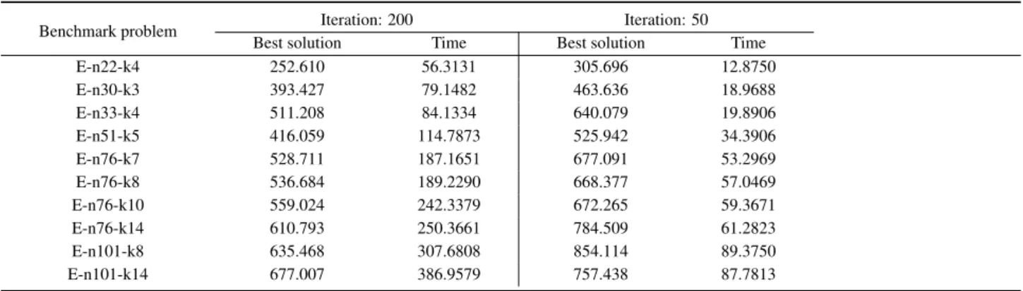
With further verification of our algorithm, standard CVRP (http://www.branchandcut.org/) is also solved by those three algorithms. For each algorithm variant, ten independent simulations are taken per benchmark. With different iteration value, the average distances are illustrated in Table 1. The convergence of distributed multi-ant algorithm (DMA) is around 100 to 150 shown in Figure 1 as the benchmark problem E-n101-k14 presented by (Christofides Nicos et al, 1979). Therefore, it is quick to find out best solutions with our algorithm. To test the determinacy, we make experiments under iteration 1000. In most benchmark problems, best solutions are almost the same as the one that under around iteration 150. To limit disturbance, iteration value of our algorithm is set as 200.
Figure 1: Computational results of E-n101-k14
In Table 2, the figures stand for best obtained fitness values (column Best solution) and average objective
val-ues of the best found feasible solutions (column Average). Compared to adaptive ant colony (AAC) and distributed ant cooperation without decomposition (DAC), DMA ob-tains better solutions to those 10 problems. Moreover, DMA runs less time (The unit of CPU time is second.). With incremental scale of problem, executed time increases slowly.
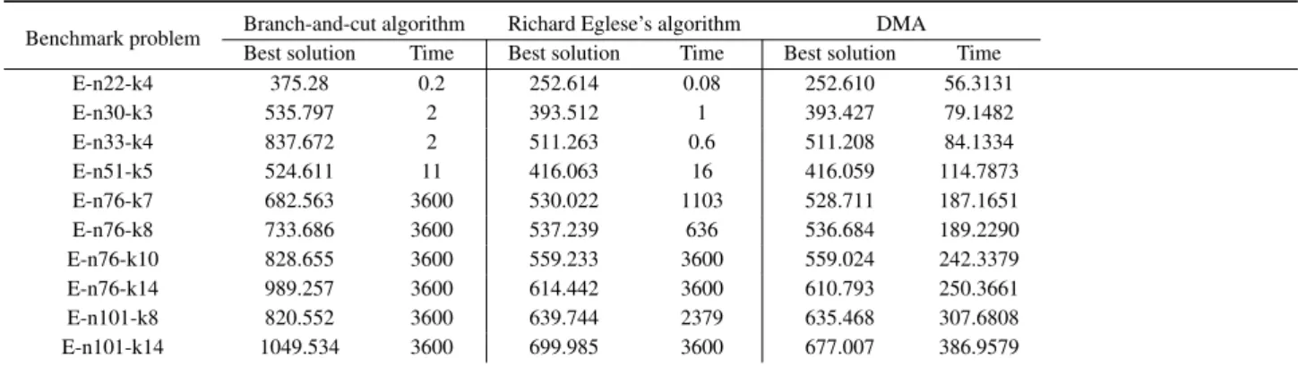
Table 3 illustrates the comparative results of best per-formances on the benchmark problem proposed by (Christofides Nicos et al,1979) according to the literature (Richard Eglese, 2009). For the experimental results of branch-and-cut algorithm and the algorithm presented by Richard Eglese, performing larger problems by exponen-tial growing costs too much time. But the performance on DMA is stable. The fluctuation of time consume is steady growth and the quality of solution is outperformed at the large scale CVRP. By reason of decomposition, DMA plays well even on large scale problems, inducing the disadvan-tage of DMA that behaviors on smaller problems also take high time consume.
4.2
Case 2: computational analysis with an
ArcView graph data
Based on the customers address and request, we try to set forth the location of cities by utilizing an GIS software, "ArcView", creating geographic data and transformed to network data containing latitude vector and longitude vec-tor. The data set of original map is loading automatically in ArcView software shown as Figure 2.
We store the digital map data of autologous city in Ar-cView. Its information is shown through digital road map utilized in several areas and edited layer structured data of spatial objects with latitude and longitude, buildings and so on. It could be found in Figure 3 amplifying Figure 2 for details. The building with red square is the distributed center and the buildings with red triangle are part of the distributed destinations. For the readability, we scale down the latitude and longitude in the digital road map by one hundred times.
Table 1: Results comparison under different iterations
Benchmark problem Iteration: 200 Iteration: 50
Best solution Time Best solution Time
E-n22-k4 252.610 56.3131 305.696 12.8750
E-n30-k3 393.427 79.1482 463.636 18.9688
E-n33-k4 511.208 84.1334 640.079 19.8906
E-n51-k5 416.059 114.7873 525.942 34.3906
E-n76-k7 528.711 187.1651 677.091 53.2969
E-n76-k8 536.684 189.2290 668.377 57.0469
E-n76-k10 559.024 242.3379 672.265 59.3671
E-n76-k14 610.793 250.3661 784.509 61.2823
E-n101-k8 635.468 307.6808 854.114 89.3750
E-n101-k14 677.007 386.9579 757.438 87.7813
Table 2: Solutions comparison with the Christofides et al. instances
Benchmark problem AAC DAC DMA
Best solution Average Best solution Average Best solution Average E-n22-k4 310.524 317.191 305.696 309.958 252.610 257.295 E-n30-k3 466.714 472.816 458.745 465.064 393.427 400.841 E-n33-k4 651.878 659.097 640.079 651.852 511.208 527.384 E-n51-k5 520.126 523.726 514.174 518.546 416.059 419.572 E-n76-k7 677.091 680.483 672.844 673.267 528.711 535.547 E-n76-k8 686.901 688.339 668.377 676.189 536.684 539.960 E-n76-k10 679.881 683.925 672.265 675.061 559.024 560.275 E-n76-k14 689.764 690.598 672.265 675.696 610.793 613.670 E-n101-k8 816.362 819.362 732.735 751.482 635.468 637.117 E-n101-k14 927.577 934.523 883.894 898.789 677.007 678.563
Figure 3: Details of digital road map
4.2.1 Results comparison
The number of places in the city is 500. In other words, the scale of CVRP is 500. Performance potential param-eter δ is 1. The simulations have undergone under three algorithms: AAC, DAC and DMA. Time consume time or-dered by AAC,DAC and DMA is 1.7514e+003 s|202.8906 s | 179.5156 s. Shortest distance by the same order is 1.4263e+004 | 1.4164e+003| 1.3541e+003. From these data, DMA gets prior performance on best solution and costs less running time. With the amount of places increas-ing, distributed multi-ant cooperation with decomposition will play more excellent. These graphs also display that DAC is easy to trap into local solution, even though DMA takes more iteration.
4.2.2 Performance potential analysis
With the scale of problem increasing, decentralized algo-rithm becomes weaker than distributed one according to its interrelate variables restrained with each others. Interaction and cooperation are critical characters of distributed model where each ant communicates through reinforcement learn-ing and renovates its next strategy even under additional places. The experiments run from two points.
In Table 4, performance potential parameter δ is 1. The scales of CVRP are 50,100,200,300,500 and 1000. Three algorithms are executed: adaptive ant colony (AAC), dis-tributed ant cooperation without decomposition (DAC) and DMA. The results are in table 4. Best solutions in DAC and AAC are trapping into local ones. While the scale is small, DMA costs more time than DAC. Because complex struc-ture process in DMA needs additional operation. However, DMA shows disadvantages in a large scale one. It takes less running time and gains better solutions than DAC and AAC.
Table 3: Best solution and time consume comparison with the Christofides et al. instances
Benchmark problem Branch-and-cut algorithm Richard Eglese’s algorithm DMA Best solution Time Best solution Time Best solution Time
E-n22-k4 375.28 0.2 252.614 0.08 252.610 56.3131
E-n30-k3 535.797 2 393.512 1 393.427 79.1482
E-n33-k4 837.672 2 511.263 0.6 511.208 84.1334
E-n51-k5 524.611 11 416.063 16 416.059 114.7873
E-n76-k7 682.563 3600 530.022 1103 528.711 187.1651
E-n76-k8 733.686 3600 537.239 636 536.684 189.2290
E-n76-k10 828.655 3600 559.233 3600 559.024 242.3379
E-n76-k14 989.257 3600 614.442 3600 610.793 250.3661
E-n101-k8 820.552 3600 639.744 2379 635.468 307.6808
E-n101-k14 1049.534 3600 699.985 3600 677.007 386.9579
Table 4: Experimental results comparison of DAC and DMA(δ=1)
amount of places Adaptive ant colony Decentralized algorithm Distributed multi-ant algorithm Best solution Cost time Best solution Cost time Best solution Cost time
Amount=50 58.76 3.4875 58.69 3.8653 56.86 4.1250
Amount=100 157.4581 25.1541 111.86 20.6354 109.22 24.7343
Amount=200 451.5714 74.1572 296.26 57.1351 235.72 50.5688
Amount=300 2874.1674 558.1547 882.29 198.7326 719.18 103.2497
Amount=500 1.4263e+004 1.7514e+004 2967.53 289.5187 1354.11 179.5156 Amount=1000 4.8417e+005 7.1541e+005 9233.76 3.5763e+003 4617.43 815.9327
plays a crucial role in distributed multi-ant algorithm.
5
Conclusion
Decomposition is usually used in decentralized model to scale down the problem into subsystems we can handle with. However, the relationship between subsystems is ig-nored easily, leading to local solution or non-solution. In this analysis, decomposition is undergoing through hybrid algorithms for large scale ofCV RPin a distributed model. Cooperation and interaction are considered and solved by distributed multi-ant algorithm. Disturbance from circum-stance is conquered by Potential function whose efficiency is verified from simulations. From the experiments, the al-gorithm has solved the large scale CV RP better and ef-ficiently. Furthermore, the next work is further control of fluctuation on solutions.
References
[1] Yuichi Nagata, Olli Braysy (2009) Edge Assembly based Memetic Algorithm for the Capacitated Vehi-cle Routing Problem,Networks, 54(4) pp. 205-215.
[2] Yeh Chung Wei (2009) Solving Capacitated Vehi-cle Routing Problem using DNA-based Computation,
Proceedings International Conference On Informa-tion Management and Engineering, pp. 170-174.
[3] Santos Luis, Coutinho Rodrigues Joao, Current John R (2009) An Improved Heuristic for the Capacitated Arc Routing Problem,Computers and Operations Re-search, 36(9) pp. 2632-2637.
[4] Borgulya Istvan (2008) An Algorithm for the Capaci-tated Vehicle Routing Problem with Route Balancing,
Central European Journal of Operations Research, 16(4) pp. 331-343.
[5] Ai The Jin, Kachitvichyanukul Voratas (2009) Par-ticle Swarm Optimization and Two Solution Repre-sentations for Solving the Capacitated Vehicle Rout-ing Problem,Computers and Industrial Engineering, 56(1) pp. 380-387.
[6] Carlos Bermudez, Patricia Graglia, Natalia Stark, Carolina Salto, Hugo Alfonso (2010) Comparison of Recombination Operators in Panmictic and Cellular GAs to Solve a Vehicle Routing Problem, Inteligen-cia ArtifiInteligen-cial, 14(46) pp. 34-44.
[7] Wang Chungho, Lu Jiuzhang (2010) An Effective Evolutionary Algorithm for the Practical Capacitated Vehicle Routing Problems,J Intell Manuf, 21(4) pp. 363-375.
[8] Gajpal Yuvraj, Abad PL (2009) Multi-ant Colony System(MACS) for a Vehicle Routing Problem with Backhauls, European Journal of Operational Re-search, 196(1) pp. 102-117.
[9] Chen Yulin, Liu Jiancheng (2002) An Tree Genera-tion Algorithm of Undirected Graphs, The Applica-tion of Computer Engineer, 38(20) pp. 115-117.
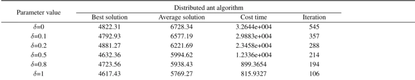
Table 5: Experimental results under differentδvalue (places=1000)
Parameter value Distributed ant algorithm
Best solution Average solution Cost time Iteration
δ=0 4822.31 6728.34 3.2644e+004 545
δ=0.1 4792.93 6577.19 2.9883e+004 357
δ=0.2 4881.27 6221.69 2.3458e+004 288
δ=0.5 4632.36 5994.62 1.2336e+004 214
δ=0.8 4723.56 5938.43 899.3654 194
δ=1 4617.43 5769.27 815.9327 106
[11] Li Yan, Yin Zongmou (2004) Techniques by Com-pound Branch and Network Ripping to Find out All Spanning Trees of an Undirected Graph,Journal of Naval University of Engineering, 16(5) pp. 74-77.
[12] Andrew Y Ng, Daishi Harada, Stuart Russell (1999) Policy Invariance under Reward Transformations: Theory and Application to Reward Shaping, ICML 1999.
[13] Moere Andrew Vande, Clayden Justin James (2005) Cellular Ants: Combining Ant-based Clustering with Cellular Automata,International Conference on Tools with Artificial Intelligence (ICTAI), pp. 177-184.
[14] Yu Xiaohu, Chen Guoan, Cheng Shixin (1995) Dy-namic Learning Rate Optimization of the Backpropa-gation Algorithm,IEEE Transactions on Neural Net-works, 6(3) pp. 669-677.
[15] Cao Xien, Chen Hanfu (1997) Perturbation Realiza-tion, Potentials and Sensitivity Analysis of Markov Processes,IEEE Transactions of Automatic Control, 42(10) pp. 1382-1393.
[16] Bagnell J Andrew, Ng Andrew (2006) On Local Re-wards and Scaling Distributed Reinforcement Learn-ing,Neural Information Processing Systems.
[17] Dietterich Thomas G (2000) Hierarchical Reinforce-ment Learning with the MAXQ Value Function De-composition,JAIR.
[18] Jiang Lingyan, Zhang Jun, Zhong Shuhong (2007) Analysis of Parameters in Ant Colony System, Com-puter Engineering and Applications, Beijing, China, 40(20) pp. 31-36.
[19] Richard Eglese (2009) The Open Vehicle Rout-ing Problem and the Disrupted Vehicle RoutRout-ing Problem: a Tale of two Problems. http:// www-eio.upc.es/seminar/09/r_eglese.pdf.