Vol. 11, No. 1, 2018, 284-298
ISSN 1307-5543 – www.ejpam.com Published by New York Business Global
Performance of linear discriminant analysis using
different robust methods
Mufda J. Alrawashdeh1,∗, Taha Radwan1,2 and Khalid Abunawas1
1 Department of Mathematics, College of Sciences and Arts, Al-Rass, Qassim University,
Kingdom of Saudi Arabia.
2 Department of Mathematics and Statistics, Port Said University, Port Said, Egypt
Abstract. This study aims to combine the new deterministic minimum covariance determinant (DetMCD) algorithm with linear discriminant analysis (LDA) and compare it with the fast mini-mum covariance determinant (FastMCD), fast consistent high breakdown (FCH), and robust FCH (RFCH) algorithms. LDA classifies new observations into one of the unknown groups and it is widely used in multivariate statistical analysis. The LDA mean and covariance matrix parameters are highly influenced by outliers. The DetMCD algorithm is highly robust and resistant to outliers and it is constructed to overcome the outlier problem. Moreover, the DetMCD algorithm is used to estimate location and scatter matrices. The DetMCD, FastMCD, FCH, and RFCH algorithms are applied to estimate misclassification probability using robust LDA. All the algorithms are expected to improve the LDA model for classification purposes in banks, such as bankruptcy and failures, and to distinguish between Islamic and conventional banks. The performances of the estimators are investigated through simulation and actual data..
Key Words and Phrases: DetMCD, FastMCD, Financial Ratios, Linear Discriminant Analysis, Orthogonalized GnanadesikanKettenring, FCH, RFCH.
1. Introduction
Linear discriminant analysis (LDA) is widely used in multivariate statistical techniques for data analysis. Rules that describe separation among groups are obtained through LDA. Variables are assumed to be normally distributed with the equal covariance matrix P
. LDA is highly sensitive to outlier observations. Hence, estimating LDA parameters using the classical approach will affect the values of parameters. Robust estimators have been proposed to limit the effects of outlier observations, and certain methods have been pre-sented to overcome the outlier problem, such as the high breakdown criterion developed by Hawkins and McLachlan [11]. Croux et al. [5] investigated the classification efficiencies
∗
Corresponding author.
Email addresses: [email protected](M. J. Alrawashdeh),taha ali [email protected](T. Radwan) [email protected](Kh. Abunawas)
of robust procedures with respect to the classical method. Rousseeuw [23] introduced the minimum covariance determinant (MCD) estimator. Rousseeuw and Driessen [25] devel-oped a new estimator called fast minimum covariance determinant (FastMCD), which is a highly robust estimator for observing outliers, to fill the gap in contaminated datasets. Todorov [27] constructed the robust Wilks lambda, which is uninfluenced by contaminated data, based on FastMCD to avoid the outlier problem. FastMCD has been applied to LDA (He and Fung [12]; Hubert and van Driessen [14]) and to different aspects of science (Hu-bert et al. [16]). FastMCD is also used in many multivariate techniques, such as the principle component analysis (Croux and Haesbroeck [7]; Hubert et al. [17]), factor anal-ysis (Pison et al. [22]), classifications, and clustering techniques. In a multivariate time series, Croux et al. [6] proposed the robust exponential smoothing of a multivariate time series to enhance the robustness of estimates for contaminated data. Different techniques and approaches use features of MCD to improve the robustness of parameter estimation. Hubert and Rousseeuw [15] presented a robust regression method for continuous situations and binary regression. Croux and Dehon [4] used robust canonical correlation. Hubert and Branden [13] introduced robustified versions of the SIMPLS algorithm. A robust multivariate calibration model was used by Hubert and Verboven [19], and a robust er-ror in variable regression was used by Fekri and Ruiz-Gazen [9]. The MCD algorithm was used for a genetic algorithm by Wiegand et al. [29]). Hubert et al. [18] used a new estimator deterministic algorithm for robust location and scatter, called determinis-tic minimum covariance determinant (DetMCD), and compared it with two estimators, namely, FastMCD and orthogonalized GnanadesikanKettenring (OGK), of Maronna and Zamar [20]. The new estimator uses the same iteration as FastMCD but does not draw random subsets, whereas FastMCD draws random subsets of size p+ 1 and is required to draw several times to obtain at least one subset that is free from outliers. DetMCD exhibited better performance and was faster than the other two estimators in estimat-ing location and scatter matrices. Olive and Hawkins [21] proposed an easy method for computing √n consistent outlier resistant estimators that can be used for inference and adopted numerous applications, including outlier detection and diagnostics, to determine whether data distribution is elliptically contoured. Olive and Ye [30] used three robust estimators of multivariate location and dispersion and then applied one of these estima-tors to create a robust method for canonical correlation analysis. One of these methods is the fast consistent high breakdown (FCH) estimator, which is fast, consistent, and highly resistant to outliers. The current work aims to combine DetMCD with LDA and compare it with the FastMCD, FCH, and robust FCH (RFCH) algorithms through simulation and actual data. Three approaches, namely, pooled covariance (PCOV), POBS, and minimum within-group covariance determinant (MWCD), are applied to improve the initial covari-ance estimate P
2. LDA
Our proposed datasets of actual and generated datapvariables measured inn observa-tions may be summarized as then×pmatrixX= (xij), wherexij denotes the expression
level ofp variables in observationsi= 1,2, . . . , nj that are sampled fromldifferent
popu-lations π1, π2, . . . , πl.
In the LDA setting, membership probability is estimated for each observation with respect to the population.
The data are sampled fromlpopulations, and each population hasnj observations,j=
1,2, . . . , l. Pl
j=1nj =nobservations can be denoted by{xij =j = 1,2, . . . , l, i= 1,2, . . . , n}. LDA has µj, Σj, and pj. µj is the mean, Σj is the covariance matrix, and pj is
the membership probability for each population πj. LDA assumes a common covariance
matrix Σ; all the parameters are unknown in practice and must be estimated from the sample data. In general, LDA parameters are estimated empirically, which leads to inac-curate values because LDA is highly influenced by outliers. All the parameters must be estimated based on robust estimators to overcome the outlier problem, thereby requiring high-performance robust estimators.
The robust LDA (RLDA) rule is expressed as follows:
Allocate x toπj if _
d
RL k (x)>
_
d
RL
j (x) for j= 1,2, . . . , g,j 6=kwith _
d
RL
j (x) =µtjΣ−1x−
1 2µ
t
jΣ−1µj+ ln(pj), (1)
where Σ is the common covariance matrix with meanµj and prior probability pj. For the
estimates of the membership probabilitypj in Eq. (1), we discuss two well-known choices.
Either pj is considered constant over all populations, thereby yielding pj = 1/L for each
j, or it is estimated as the relative frequencies of the observations in each group, thereby yieldingpj =nj/n.
If ˜nj denotes the number of non-outliers in group j and ˜n=Plj=1˜nj, then the
mem-bership probability is robustly estimated as follows:
_
P
RL
j =
˜ nj
˜
n. (2)
3. DetMCD estimator
The DetMCD algorithm starts by standardizing data to obtain the standardized Z. Each variableXjwill be subtracted from the median and divided by theQnscale estimator
(Rousseeuw and Croux [24]). This standardization enables the equivariance of algorithm location and scale. The standardized dataset is denoted by the n×p matrixZ with row zt
i (i= 1,2, . . . , n) and column zj (j= 1,2, . . . , p).
Six initial estimates of µk(z) and Σk(z), where (k = 1,2, . . . ,6), represent the mean
and covariance matrix, respectively, of Z. EachSk estimator computes the covariance or
correlations of matrixZ.
4. Six initial scatter estimators
(i) S1 is computed by the hyperbolic tangent of each column of Z, Yj = tanh(Zj)
for j = 1, . . . , p. This bounded function reduces the effect of large coordinate-wise outliers. Then, the classical correlation matrix of Y is computed to obtain S1 =corr(Y).
(ii) S2is computed by determiningRj, the rank of each columnZj. Then,S2 =corr(R),
which is the Spearman correlation matrix ofZ.
(iii) S3 is the normal score computed from Rj; that is,Tj =φ−1((Rj−1/3)/(n+ 1/3)),
whereφ(·) is the normal cumulative distribution function. Then,S3 =corr(T). (iv) S4is the scatter estimator computed based on the spatial sign covariance matrix
(Vi-suri et al. [28]) and is defined aski =zi/kzikfor alli. Then, S4 = (1/n)Pni=1kikTi .
(v) S5 is the first step of the BACON algorithm (Billor et al. [2]). The {n/2} stan-dardized observationzi has the smallest norm and is used to compute the mean and
covariance matrix.
(vi) A scatter estimate is the raw version of the OGK estimator. Form(·), s(·), and the median, Qn is used for simplicity.
After standardizing the data and obtainingc, three steps are completed to obtain the covariance and mean of DetMCD.
(i) The matrix E of the eigenvectors ofSk is computed and B =ZE is applied.
(ii) The center ofZis estimated using Σk(Z) =ELET, whereL=diag(Q2n(B1), . . . , Q2n(Bp)).
(iii) The covariance of Z is estimated using sphere data, the coordinate-wise median is applied and transformed back,µk(Z) = Σ
1/2
k (med(ZΣ
1/2
For all the six estimatesSk, (µk(Z),Σk(Z)) is used to compute the statistical distance, as
follows:
dik =d(µk(Z),Σk(Z)). (3)
For the initial estimate k,h◦ = [n/2] observations are taken with the smallestdik. Then,
the statistical distances d∗ik for h◦ observations are computed. All h observations xi are
calculated with the smallestd∗ik for all the six estimates. The final step is the application of the concentration step (C-step) until convergence. The estimate with the smallest determinant is called the raw DetMCD. The final DetMCD is obtained by applying the reweighted FastMCD algorithm.
As previously mentioned, RLDA is constructed based on the DetMCD algorithm. RLDA is derived by inputting the location and scatter matrices obtained based on the DetMCD algorithm into LDA, as follows:
_
d
DetM CD
j (x) =µtjΣ
−1x−1 2µ
t jΣ
−1µ
j+ ln(pj). (4)
Outliers in the data are flagged to robustify the location and scatter matrices. The ro-bust distance for each observation xij is computed from the group πj to estimate the
membership probability, as follows:
RDDetM CDij = q
(xij −µˆj)tΣ−1(xij−µˆj). (5)
Then,xij is considered the outlier observation if and only if
RDij >
q χ2
p,0.975. (6)
Finally, the membership probability P_
DetM CD
j can be obtained using Formula (8) after
applying the DetMCD estimator that is defined as follows:
_
P
DetM CD
j =
˜ nj
˜
n. (7)
5. FastMCD
The main feature of the FastMCD algorithm is the C-step, where det(Σnew) det(Σold)
with equality if det(Σnew) = det(Σold) (Rousseeuw and Driessen [25]). The application
mean and covariance matrix.
The same approach applied to the DetMCD algorithm to obtain RLDA, andpR
j is applied
to the FastMCD algorithm, which is defined as follows:
_
d
F astM CD
j (x) =µtjΣ−1x−
1 2µ
t
jΣ−1µj+ ln(pj). (8)
The membership probabilitypj of the robust distance is defined as follows:
RDF astM CDij = q
(xij −µˆj)tΣ−1(xij−µˆj). (9)
If xij is used to consider the outliers in Formula (6), then the membership probability of
the FastMCD estimator is expressed as follows:
_
P
F astM CD
j =
˜ nj
˜
n. (10)
6. FCH
The most practical estimators are used as a sequence of n trial fits called initial es-timator, (µ1,Σ1),(µ2,Σ2), . . . ,(µn,Σn). The initial estimator (µi,Σi) that minimizes the
evaluation criterion will be used in the final estimator. The initial estimator obtained by the generated trial fits is called start. Then, the C-step technique will be applied.
We let (µ0,i,Σ0,i) be the ith start and all nMahalanobis distances Di(µ0,i,Σ0,i). The
classical estimator (µ1,i,Σ1,i) is computed from cn ≈ n/2 cases that correspond to the smallest distance. We continue the iteration for k steps, thereby resulting in the follow-ing sequence: (µ0,j,Σ0,j)(µ1,j,Σ1,j),(µ2,j,Σ2,j), . . . ,(µk,j,Σn,k). The values of cn and k
depend on the C-step estimator. The value of k in the FastMCD estimator is 500, with randomly drawn elemental sets of p+ 1 cases as the start. The initial estimator with the smallest determinant is used for the final estimator. Hawkins and Olive [10] have a similar estimator.
The FCH estimator uses two estimators. The first estimator is the DGK estimator (De-vlin, Gnanadesikan, and Kettenring [8]), which uses the classical estimator as the start. The second estimator is the median ball (MB) estimator, where the classical estimator is computed from cases withDi(M ED(X), Ip)≤M ED(Di(M ED(X), Ip)) as the start, and
M ED(X) is the coordinate-wise median. In case the DGK location estimator obtains a greater Euclidean distance fromM ED(X) than half of the data, then FCH will apply the median ball estimator. We let (µ0,Σ0) be the initial estimator used. Then, the estimator (µ,Σ) takes µ0 =µ and Σ = M ED(D2i(µ0,Σ0))
χ2
p,0.5 Σ0, where χ
2
p,0.5 is the 50th percentile of the chi-square distribution with p degrees of freedom.
and is expressed as follows:
_
d
F CH
j (x) =µtjΣ
−1x−1 2µ
t jΣ
−1µ
j+ ln(pj). (11)
The membership probabilitypRj of the robust distance is defined as follows:
RDF CHij = q
(xij −µˆj)tΣ−1(xij−µˆj). (12)
If xij is used to consider the outliers in Formula (6), then the membership probability of
the FCH estimator is expressed as follows:
_
P
F CH
j =
˜ nj
˜
n. (13)
7. Simulation study
In this section, different algorithms are applied to estimate the LDA parameters using small and medium datasets. The simulation is similar to that of He and Fung [12]. All the estimators are used in the raw and reweighted versions to obtain the initial mean and covariance matrix, that is,µ0and Σ0, respectively. This estimator will yield a discrim-inate rule based on robust dRLj (x, µ0,Σ0). Then, the reweighted version will be obtained based on the robust distances (Rousseeuw and van Zomeren [26]), as follows:
RDij =
q
(xij −µˆj,0)tΣ0−1(xij −µˆj,0). (14)
For each observation in group j,
wij =
(
1 if RDij ≤
q χ2p,0.975
0 otherwise . (15)
Three approaches presented by Hubert and van Driessen [14] are adopted to estimate the means and common covariance matrices for all the groups with raw and reweighted versions. The same approaches have been used to compare the robust and classical LDA (Alrawashdeh et al. [1]). These approaches are also applied to the estimators of the FastMCD, DetMCD, and FCH algorithms.
The first approach is direct and has been applied by Chork and Rousseeuw [3], where µj and Σj are obtained by pooling the covariance matrix Σj,Algorithm as follows:
_
ΣP COV=
Σlj=1nj _
ΣjAlgorithm Pl
j=1nj
This approach will be denoted by PCOV for the raw version and PCOV-W for the reweighted version.
For the second approach, the concept is based on pooling the observations instead of the group covariance matrices. This approach was proposed by He and Fung [12], who used an S-estimator, and adopted by Hubert and van Driessen [14]. The number of groups in the simulation and that for other groups will follow the same pattern to simplify the notation of the three groups. In the three samplesA= (a11, a21, . . . , an1,1),B = (b12, b22, . . . , bn2,2),
andC= (c13, c23, . . . , cn3,3),µA,µB, andµC are the location estimators of the populations
in the reweighted FastMCD. The pooled and shifted observations are expressed as follows:
Z = (z1, z2, . . . , zn) = (a11−µA, a21−µA, . . . , an1,1−µA, b12−µB, b22−µB, . . . , bn2,2−µB
, c13−µC, c23−µC, . . . , cn3,3−µC).
The covariance matrix Σz is estimated as the reweighted FastMCD of the scatter matrix
of z. The location µz is estimated by the MCD estimator. µz is used to upgrade the
locations of µj to obtain _
µa=µa+µz, _
µb=µb+µz, and _
µc=µc+µz. The observations
in this approach are pooled instead of the covariance matrices. Hence, RLDA is denoted by POBS for the raw version and POBS-W for the reweighted version.
The third method is a combination of the two previous methods. This method aims to de-rive a fast approximation of the MWCD criterion (Hawkins and McLachlan [11]). Instead of performing the same adjustment for each group, h is identified from all observations with set size n, where the covariance matrix ΣH of h has a minimal determinant. Then,
the covariance matrix ofH (h out ofn) is obtained. The approach for the three groups is as follows.
(i) The canters of the groups are estimated.
(ii) The observations are shifted and pooled to obtainz’s that are the same as those in the second approach using the FastMCD estimator.
(iii) Let H beh out ofn based on the minimized FastMCD estimator.
(iv) The subsetHis partitioned intoHA,HB, andHC, which contain observations from
A,B, and C, respectively.
(v) The mean of all the groups is estimated as µA,µB, andµC.
8. Simulation result
Through the simulation study, we compare the performances of the three approaches in estimating the initial values for the mean and covariance matrix and then apply the obtained values to FastMCD, DetMCD, and FHC to obtain the misclassification proba-bilities. We use the raw and reweighted versions for all the algorithms. The RLDA rule is applied using settings similar to those in the study of He and Fung [12]:
A⇒π1 : 400N3(0, I) π2 : 400N3(1, I)
B ⇒π1 : 400N3(0, I) + 50N3(5,(1/0.252)I) π2 : 400N3(1, I) + 50N3(−4,(1/0.252)I) C ⇒π1 : 80N3(0, I) + 20N3((1,(1/0.252)I)
π2 : 80N3(1, I) + 20N3((−1,(1/0.252)I) D⇒π1 : 200N3(0, I) + 25N3((1,(1/0.075)I) π2 : 200N3(1, I) + 25N3((−1,(1/0.075)I) E ⇒π1 : 300N3(0, I) + 10N3(5,0.252I)
π2 : 150N3(1, I) + 5N3(−10,0.252I) ,
whereIis the 3D identity matrix, the groups labeled as A, B, C, D and E, each group has to different cases π1 andπ2. The membership probability is calculated based on Formula (8) forl in consideration of the two algorithms. The classification rule (Eq. (1)) is robustified as the Fisher discriminant rule, which expressed as follows:
x∈π1if(_µ1 −
_
µ2)tΣ−1(x−(_µ 1 −
_
µ2)/2)>0 (17)
and x∈π2 otherwise.
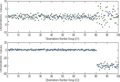
Figure 1 presents only the first 100 observations from the groups of Case C. The figure shows the scatter of data in Case C, in which both groups have outliers. The effects of the outliers on data homogeneity and on the parameters of the discriminate rules that will be used to estimate values are clearly shown. Graphs C1 and C2 show a cut and abnormal spread for the observations.
Figure 1: Observations Number Group of C1 and C2
the efficiency of the discriminate estimates compared with the other two estimators. In the two versions, the DetMCD algorithm obtains more accurate values for MP.
The DetMCD estimator values are more accurate and less than 10% for all the cases in the simulation. The data in Case A contain an uncontaminated dataset and the esti-mated values are comparable for both versions performance groups, except the MWCD for FastMCD and RFCH. The datasets for Cases B, C, D, and E are generated from con-taminated datasets with different percentages of outliers for each case and group. Groups A and B are generated with the same number of observations. Case B is generated with 25% outlier observations. The outliers influence the estimator rules, where the estimated values of case B are 0.0751 and 0.0559 for the raw and reweighted versions, respectively,
Table 1: Mean µ for the misclassification probabilities of the RLDA rules for 500 replications based on the DetMCD, FastMCD, and FCH algorithms for the raw version
Algorithm FastMCD DetMCD FCH
Version Raw Raw Raw
Approach PCOV POBS MWCD PCOV POBS MWCD PCOV POBS MWCD
Table 2: Mean µ for the misclassification probabilities of the RLDA rules for 500 replications based on the DetMCD, FastMCD, and FCH algorithms for the reweighted version
Algorithm FastMCD DetMCD RFCH
Version Reweighted Reweighted Reweighted
Approach PCOV-W
POBS-W
MWCD-W
PCOV-W
POBS-W
MWCD-W
PCOV-W
POBS-W
MWCD-W Group A 0.1954 0.1956 0.3937 0.0197 0.0089 0.0923 0.2084 0.1934 0.3826 Group B 0.3188 0.3192 0.3227 0.0751 0.0559 0.1246 0.3385 0.3248 0.3354 Group C 0.3703 0.3713 0.5351 0.0835 0.076 0.1185 0.4073 0.3943 0.5324 Group D 0.2805 0.2812 0.5405 0.082 0.0782 0.1073 0.2854 0.2793 0.5523 Group E 0.2907 0.2908 0.3699 0.0237 0.0232 0.1202 0.3054 0.3094 0.3893 based on DetMCD. The estimated values for Cases A, B, C, D, and E are comparable, except for Case A, which is determined to have the best value of 0.0089 for the reweighted version using the POBS approach. From all the contaminated datasets and cases, E is the most accurate because it is close to the uncontaminated dataset in Case A, with a differ-ence of approximately 0.0144 and 0.0143 for the raw and reweighted versions, respectively. By contrast, the MWCD approach performs poorly with the DetMCD algorithm, whereas the other two approaches perform better in both versions. The results of FCH exhibit better performance in Case A, which indicates better performance at the uncontaminated dataset in the raw version, but FastMCD was better at the reweighted version for all the approaches. By contrast, the performances of the PCOV and POBS approaches are approximately close to each other at the FastMCD and FCH estimators for the raw and reweighted versions, but MWCD performs poorly compared with the other approaches.
Table 3: Misclassification probability estimates for DetMCD, FastMCD, and FCH for the raw version RLDA rules based on actual data (financial ratios for Islamic and conventional banks in Malaysia)
Algorithm FastMCD DetMCD FCH
Version Raw
Approach PCOV POBS MWCD PCOV POBS MWCD PCOV POBS MWCD
MP 0.214 0.1845 0.0352 0.0182 0.06 0.2227 0.217 0.1954 0.0932
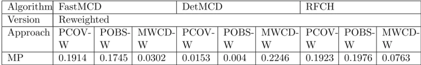
Table 4: Misclassification probability estimates for DetMCD, FastMCD, and FCH for the reweighted version RLDA rules based on actual data (financial ratios for Islamic and conventional banks in Malaysia)
Algorithm FastMCD DetMCD RFCH
Version Reweighted Approach
PCOV-W
POBS-W
MWCD-W
PCOV-W
POBS-W
MWCD-W
PCOV-W
POBS-W
MWCD-W
MP 0.1914 0.1745 0.0302 0.0153 0.004 0.2246 0.1923 0.1976 0.0763
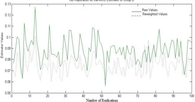
Figure 2 presents the replications for the first 100 times out of the 500 replications. The figure describes the values of the misclassification probabilities of the discriminate rules based on the DetMCD estimator. The disparity of the misclassification values is shown, particularly for the raw version, where the difference between the minimum and maximum values is considerable compared with that for the reweighted version. In terms of the accuracy of the versions of the DetMCD estimator, the reweighted version is more accurate and efficient than the raw version.
9. Example of actual data: Islamic and conventional banks in Malaysia
The financial ratios of Islamic and conventional banks in Malaysia are used as actual data. A total of 271 observations from banks for the period of 2003–2011 are used, where 96 observations are from Islamic banks and 175 observations are from conventional banks. The dataset has 23 financial ratios (variables). The data were collected from the Bankscope database, which converts financial data according to common international standards to facilitate comparisons. RLDA is applied using the three estimators. All the estimators have been used with the three approaches described in the previous section. The results are presented in Table 3 and Table 4 for the raw and reweighted versions, respectively.
10. Conclusion
In this study, we investigated the difference in efficiency among three estimators, namely, DetMCD, FastMCD, and FCH, of location and scatter for RLDA, in which the groups have a common covariance matrix. DetMCD, FCH, and FastMCD are compared based on three approaches to estimate the common scatter matrix. Membership probabil-ities in a robust structure are estimated by considering only observations of non-outliers. Then, misclassification probabilities for the data are obtained and set into two groups of datasets.
The results of the simulation clearly showed how the robust structure was better and how the DetMCD algorithm for the robust and non-robust structures was better than the FastMCD and FCH algorithms. For the robust structure, DetMCD performed better and was unaffected by outliers. The DetMCD algorithm achieved high efficiency for RLDA and was more accurate than the FastMCD and FCH algorithms. We applied the RLDA rules on actual datasets based on the two algorithms.
The DetMCD algorithm performed well compared with the FastMCD and FCH rithms; RLDA with DetMCD achieved the highest efficiency. Thus, the DetMCD algo-rithm increased the accuracy and performance of the LDA model, which indicates more advantages to utilize the model with highly robust estimations. On the basis of the results of the simulation and actual data, the DetMCD algorithm can be used with RLDA in financial research to predict firm failure, bankruptcy, and company distress. It also has applications in other fields, e.g., recognitions.
Acknowledgements
The authors gratefully acknowledge Qassim University, represented by the Deanship of Scientific on the material support for this research under the number (1475) during the academic year 1437 AH/2016 AD.
References
[1] Mufda Jameel Alrawashdeh, Shamsul Rijal Muhammad Sabri, and Mohd Tahir Is-mail. Robust linear discriminant analysis with financial ratios in special interval.
Applied Mathematical Sciences, 6(121):6021–6034, 2012.
[2] Billor, Nedret, Ali S Hadi, and Paul F Velleman. Bacon: blocked adaptive compu-tationally efficient outlier nominators. Computational Statistics and Data Analysis, 34(3):279–298, 2000.
[4] Croux, Christophe, and Catherine Dehon. Analyse canonique base sur des estimateurs robustes de la matrice de covariance. Revue de statistique applique, 50(2):5–26, 2002. [5] Croux, Christophe, Peter Filzmoser, and Kristel Joossens. Classification efficiencies
for robust linear discriminant analysis. Statistica Sinica, 18(2):581–599, 2008. [6] Croux, Christophe, Sarah Gelper, and Koen Mahieu. Robust exponential smoothing
of multivariate time series.Computational Statistics and Data Analysis, 54(12):2999– 3006, 2010.
[7] Croux, Christophe, and Gentiane Haesbroeck. Principal component analysis based on robust estimators of the covariance or correlation matrix: influence functions and efficiencies. Biometrika, 87(3):603–618, 2000.
[8] Devlin, S. J., Gnanadesikan, R., Kettenring, and J. R. Robust estimation of dispersion matrices and principal components. Journal of the American Statistical Association, 76(374):354–362, 1981.
[9] Fekri, M, and Anne Ruiz-Gazen. Robust weighted orthogonal regression in the errors-in-variables model. Journal of the American Statistical Association, 88(1):89–108, 2004.
[10] Hawkins, D.M., Olive, and D.J. Improved feasible solution algorithms for high break-down estimation. Computational Statistics and Data Analysis, 30:1–11, 1999. [11] Hawkins, Douglas M, and Geoffrey J McLachlan. High-breakdown linear discriminant
analysis. Journal of the American statistical association, 92(437):136–143, 1997. [12] He, Xuming, and Wing K Fung. High breakdown estimation for multiple
popula-tions with applicapopula-tions to discriminant analysis. Journal of Multivariate Analysis, 72(2):151–162, 2000.
[13] Hubert, Mia, and K Vanden Branden. Robust methods for partial least squares regression. Journal of Chemometrics, 17(10):537–549, 2003.
[14] Hubert, Mia, and Katrien Van Driessen. Fast and robust discriminant analysis. Com-putational Statistics and Data Analysis, 45(2):301–320, 2004.
[15] Hubert, Mia, and Peter J Rousseeuw. Robust regression with both continuous and binary regressors.Journal of Statistical Planning and Inference, 57(1):153–163, 1997. [16] Hubert, Mia, Peter J Rousseeuw, and Stefan Van Aelst. High-breakdown robust
multivariate methods. Statistical Science, 23(1):92–119, 2008.
[18] Hubert, Mia, Peter J Rousseeuw, and Tim Verdonck. A deterministic algorithm for robust location and scatter. Journal of Computational and Graphical Statistics, 21(3):618–637, 2012.
[19] Hubert, Mia, and Sabine Verboven. A robust pcr method for highdimensional regres-sors. Journal of Chemometrics, 17(89):438–452, 2003.
[20] Maronna, Ricardo A, and Ruben H Zamar. Robust estimates of location and disper-sion for high-dimendisper-sional datasets. Technometrics, 44(4):307–317, 2002.
[21] David J. Olive and Douglas M. Hawkins. Robust multivariate location and dispersion.
Southern Illinois University and University of Minnesota, 2010.
[22] Pison, Greet, and et al. Robust factor analysis. Journal of Multivariate Analysis, 84(1):145–172, 2003.
[23] Rousseeuw and Peter J. Least median of squares regression. Journal of the American statistical association, 79(388):871–880, 1984.
[24] Rousseeuw, Peter J, and Christophe Croux. Alternatives to the median absolute deviation. Journal of the American Statistical Association, 88(424):1273–1283, 1993. [25] Rousseeuw, Peter J, and Katrien Van Driessen. A fast algorithm for the minimum
covariance determinant estimator. Technometrics, 41(3):212–223, 1999.
[26] Rousseeuw, Peter J, and Bert C Van Zomeren. Unmasking multivariate outliers and leverage points. Journal of the American Statistical Association, 85(411):633–639, 1990.
[27] Todorov and Valentin. Robust selection of variables in linear discriminant analysis.
Statistical Methods and Applications, 15(3):395–407, 2007.
[28] S. Visuri, H. Oja, and V. Koivunen. Sign and rank covariane matrices. J. Statist. Plann. Inference, 91:557575, 2000.
[29] Wiegand, Patrick, Randy Pell, and Enric Comas. Simultaneous variable selection and outlier detection using a robust genetic algorithm. Chemometrics and Intelligent Laboratory Systems, 98(2):108–114, 2009.