УДК 629.4
B. FISHER, Dipl.-Ing., ArgeCare, Berlin, (Germany) R. MENSSEN, Dipl.-Ing., ArgeCare, Berlin, (Germany)
O. MARKOVA, Dr. (Cand.), ITM NANU, Dnepropetrovsk, (Ukraine) H. KOVTUN, Dr. (Cand.), ITM NANU, Dnepropetrovsk, (Ukraine)
DESIGN SIMULATION TO PASS TESTS FOR ACCEPTANCE
AS DEFINED IN prEN14363 OR UIC518
Щоб бутиупевненим, щозновурозробленийістворений рейковийекіпажуспішнопройдеприймальніви
-пробування, необхідно досліджувати його поводження за допомогою комп'ютерного моделювання. Оцінка впливузмінирізнихпараметрівдозволяєтакожоптимізуватирозміриіпараметриконструкції. Уроботідеталь
-ноописанінеобхіднідляпроведенняоцінкидинамічнихякостейекіпажа варіантимоделювання, показано, які параметривизначаютьточністьрішенняпоставленоїзадачі.
Чтобы быть уверенным, что вновь разработанный и созданный рельсовый экипаж успешно пройдет приемочные испытания, необходимо исследовать его поведение с помощью компьютерного моделирования.
Оценка влияния изменения различных параметров позволяет также оптимизировать размеры и параметры конструкции. Вработедетальноописанынеобходимыедляпроведенияоценкидинамическихкачествэкипажа вариантымоделирования, показано, какиепараметрыопределяютточностьрешенияпоставленнойзадачи.
Introduction
International rail traffic is possible due to interna-tional standards and acceptance procedures. To re-duce the needed time and money to pass the tests de-sign calculations are very helpful. Powerful rail ve-hicle calculation tools as ADAMS/Rail, MEDYNA, SIMPACK, VAMPIRE and others were developed and verified during the last years.
More important than MBS-algorithms is a realis-tic modelling of design elements as spring, damper, bump stop, friction element with their non-linear characteristics and last but not least modelling of wheel rail contact. An accurate result is more impor-tant than savings in calculation time.
The standards represent the experience of Euro-pean railways in testing for acceptance of the run-ning characteristics of vehicles. Simplified methods are also included to reduce expense of tests. This pa-per deals with the main aspects only of limits and procedures given in the standards.
Aim of Design Optimisations
The aim of a design is to build a vehicle with a good performance at a low price. Good running be-haviour and low life cycle costs are important as-pects for a decision about design parameter. Forces between wheel and rail, wear of profiles, comfort in the car body has to be optimised running on straight
tracks with maximal velocity and through curves with high or low cant deficiencies.
Full tests, partial tests and simplified measure-ment method
The necessary amount of tests, methods and sig-nals which have to be measured is depending on characteristics of the vehicle as axle load, velocity and knowledge of the design. Simulation allows in-vestigating the dynamic behaviour and all values of the vehicle in detail. This opportunity should be used to find a good solution during the design process. The possibility of simplified measurement methods are not dealt with further as design calculations should not be restricted to these values. Information and knowledge about the vehicle performance are as well less with fewer values evaluated.
Assessment values
Only the assessment values of the normal meas-urement procedure are mentioned in the following. The values looked for are sorted according the rea-son as:
– running safety; – track load;
– ride characteristics.
Sum of guiding forces
∑
Ymax is the safety-critical limit for track shifting. The given limits are for a standard ballasted track with timber sleepers.) 3 / 2 10 ( 1 lim
max, k Qo
Y = ∗ +
Σ in kN, (1)
o
Q
2 is the static wheelset load in kN. The factor k1 is depending on the type of vehicle:
1
k = 1.00 for locomotive, multiple units and, passenger coaches,
1
k = 0.85 for freight wagons.
The value of axle box force H is equivalent to
∑
Y but low pass filtered due to unsprung mass and primary suspension.Quotient of guiding force and wheel force (Y/Q)max is the safety-critical limit of derailment for the quotient of a leading wheel.
lim max, ) /
(Y Q < 0.8 (2)
on track.
There is no way to calculate Y from the H force measurement as there are wheelset internal forces as result of lateral friction.
Instability criterion is described with
2 / lim max, lim , Y
Yrms =Σ
Σ . (3)
The random mean square value of a section has to be less than half of the track shift limit.
Limit values of track loading The quasi-static guiding force is limited to
lim ,
qst
Y < 60 kN (4)
and the quasistatic wheel force is limited to
lim ,
qst
Q < 145 kN (5)
both excluding transition sections.
lim max,
Q = 90 + Qo in kN (6)
depending on maximum of permissible speed of the vehicle the force is limited to
lim max,
Q < 160 kN … 200 kN , (7) v < 160 km/h … 300 km/h. (8)
These values take account of rails with a weight per meter > 46 kg and the minimum value of rail strength of 700 N/mm².
Limiting values of ride characteristics The limiting values of ride characteristics are ac-celerations in the vehicle body. They are measured in lateral and vertical directions in the centre and over the running gears. Maximal values and mean square values are limited depending on the type of vehicle.
Simulation of Stationary and ‘On Track’ Tests
Simulation makes it possible to study dynamic behaviour of the vehicle in detail. In simulation it is easy to define any kind of track and to analyse the vehicle for all track cases which have to be passed in future time.
Stationary Tests
The vehicle has to show in stationary tests that there is no risk of derailment, to exceed the kine-matic envelope and loss of contact of the pantograph to the overhead wire.
Safety against derailment
The test conditions have been developed by ERRI and documented in several reports [3]. They are carried out on twisted test track with a radius of R = 150 m and changing cant from 45 mm to -45 mm within 30 m to get a twist of +3 %o.
The wheel with the lowest load has to run in leading position on the outer rail. The test twist is be-tween 3 %o and 7 %o depending on the bogie wheel
base and the distance 2a between the bogies.
lim
g = min(7.0; 20/2a +2.0) (9)
If test track twist is greater than 3 %o this have to be done using shims in the suspensions.
This test has to be calculated using time integra-tion methods. The vehicle has to pass the test track with a speed lower than 10 km/h. Possible hysteresis within suspensions has to be modelled carefully. Rails must be in dry condition. Figure 1 shows the minimum of desired values of coefficient of friction
τ =
µ . Calculations should be done with higher co-efficient of friction to simulate the worst case µ ~ 0.4…0.5.
The tests conditions have been developed by British Rail and were partly used in the so-called Manchester benchmark track case 1 [6]. A linear dip of 20 mm over 6 m has to be put at the high rail in the run-off transition and a body-bogie yaw torque should act additionally.
Fig. 1. Coefficient of friction measured by UIC [3]
Sway characteristic
The vehicles have to run inside a kinematic enve-lope and so they are not allowed to move freely. The test is done on a canted track to simulate curving, side wind etc. The calculation determines quasista-tionary equilibrium.
‘On Track’ Tests
On track tests investigate characteristics of a ve-hicle with regard to the interaction to the track layout and rail deviations. Test zones are track sections with the characteristic:
– straight;
– large curves R > 600 m;
– small curves 600 m > R > 450 m or – very small curves 450 m > R > 250 m.
The length of sections is 70 m to 500 m accord-ing to track layout and speed.
Track geometry quality
The track quality is based on track maintenance criteria and a definition is given in the standard prEN14363:
a) quality level QN 1:
necessitates observing a track section or taking main-tenance measures within the frame of normal opera-tions scheduling,
b) quality level QN 2:
necessitates taking short-term maintenance measures, c) quality level QN 3:
characterizes track sections which do not exhibit the usual track geometry quality. Quality level QN 3, however, does not represent the most adverse but still tolerable maintenance status.
The standards forced to do tests on tracks with quality QN 2 with 10 % of the total length of test sections. So this quality has mainly to be used for simulation as that is normally the most critical condi-tion.
The quantities of track geometry deviations de-pend on line speed. The characteristic values are evaluated in a bandwidth of 3 m to 25 m wavelength. This is due to the standard performance of measure-ment devices of track geometry. But to get realistic simulation results the geometry has of cause to be used with a wider range of wavelength. The interest-ing excitation frequency normally is between 0.3 to 30 Hz. The conversion into wavelength L is done with the velocity.
v f
L= ∗ (10)
with f – frequency in Hz and v – velocity in m/s.
Definition of deviation with PSD
The dependency of amplitude from frequency or wavelengths Ω in rad/m is defined by a power spec-tral density PSD-function [5]:
) (
* )
( 2 2 2 2 2
r c
c A S
Ω + Ω Ω + Ω
Ω ∗
= in
m rad
m
/ ² (11)
with lateral A = 0,6125 and vertical A = 1,08 in m
rad∗ for high level and
c
Ω = 0,8426 and Ωr= 0,0206 in rad∗m.
Ω in rad∗m
Example 1. Realisation of rail deviations, line speed 80 km/h.
The lateral displacements of right and left rails are shown along the track in figure 2. The values of the light grey curve are filtered in the range between 3 m to 25 m to get the quality level. The dark curve represents the values in a wavelength between 1 m and 70 m.
pass filtered values in a range of 25 m to 3 m wave-length in the plot over the distance in Figure 3 [4].
Fig. 2: Realisation of rail deviations [4]
Example 2. Evaluation of measured track with line speed 250 km/h.
Fig. 3: Evaluation of measured rail deviations [4]
Conicity, wheel rail profiles
The standard gives only some hints about profiles of wheel and rail. The running characteristics of a vehicle are influenced by the combination of wheel and rail profiles. One describing function is the so-called conicity. This is a function of the difference of left and right wheel roll radii at lateral amplitudes. The prEN 14363 defines the so called equivalent conicity tan(γe).
For a given wheelset running on given track it equals the tangent of the taper angle of a tapered pro-file wheelset whose transverse movement has the same wavelength of kinematic yaw as the wheelset under consideration.
The wheel profiles of a wheelset are combined with rail profiles (including the inclination) and the track gauge.
Conicity values are found on freight lines up to
)
tan(γe =0.8 due to pure maintenance or narrow gauge. And on high speed line there is a conicity up to tan(γe)=0.3 or even 0.4.
The standard defines to measure wheel profile in service to analyse if conicity has changed. Calcula-tions are necessary to derive if profile wear changes conicity during service as shown in Figure 4.
Design simulations
To design a vehicle with good performance and to know test results in advance a lot of computer simulations have to be done.
Fig. 4: Change of conicity due to profile wear (RSGEO)
Natural behaviour
The natural behaviour of a rail vehicle depends on the speed it is running. Hunting mode and fre-quency depends on the velocity of the vehicle. Some of the eigen-modes change with speed quite a lot, other only slightly. The ratio of damping and fre-quency of some modes are shown in Figure 5. If damping falls below a certain value (in theory zero) the so-called critical speed is reached.
Fig. 5: Damping and frequency depending on speed
Figure 6 shows as function of speed the frequen-cies of some body modes and the speed depending hunting mode.
Hunting phenomena occurs due to selfexciting effects in wheel rail contact. Below the so-called critical speed movements of wheelsets are damped; above they are increasing with the behaviour of non-linear systems to approach a limit cycle.
Fig. 6: Frequencies as a function of speed
Rail irregularities will normally stabilize the sys-tem. Which means calculated critical speed on smooth track is on save side for the system.
This limit depends on:
– coefficient of friction between wheel and rail; – conicity;
– suspension parameter of the vehicle; – masses, etc.
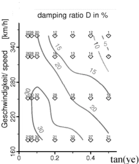
Therefore an evaluation is done to find the speed depending eigen-mode which has the lowest damp-ing ratio. If an additional parameter is changed low-est ratios damping ratio can be shown in a 3D-plot or contour plot – stability chart. Lines of same damping are plotted against conicity tan(γe) and speed in Figure 7.
Beside conicity other parameters of the vehicle can be changed as e.g. lateral primary stiffness of wheelsets.
Another method to determine critical speed is to investigate self-excited movement of the vehicle. A non-linear integration is done with changing veloc-ity. At high speed hunting mode is initiated either by self or forced excitation. The hunting movement which can show different shapes as velocity is de-creased must die out. When altitudes on undisturbed track become zero, the speed is called critical speed. The critical speed of two design variants is shown in Figure 8.
Fig. 7: Results of linear stability simulation
Fig. 8: Results of non-linear stability simulation (MEDYNA)
The critical speed rises from 50 to 95 m/s using an improved bogie design fitted with a radial arm.
Vehicle interaction with track
The running behaviour describes the characteris-tics of a vehicle with regard to the interaction be-tween vehicle and track. Track layout is defined as:
– straight track with variation of speed; – curved track;
– large curves with speed up to maximal velocity; – small and very small curves with unbalanced lateral accelerations up to maximal cant deficiency.
Rail deviations have to be selected according the speed.
All these simulations should be done with varia-tions of:
– wheel and rail profiles;
– worn profiles / change in conicity.
Behaviour of vehicle with very strong side wind High-speed vehicle get in trouble running through very high side dusts. This occurs running on embankments or over bridges. Such situation has to be investigated calculating such situations with lat-eral forces acting on the car body.
Optimisation of vehicle performance The performance of rail vehicle mainly depends on:
– stiffness of primary and secondary suspensions, – damping parameter,
– parameter of additional devices to get better stability or curving e.g. using the radial arm design of Dr. Scheffel.
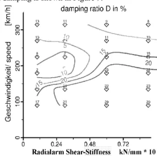
A design optimisation is shown using example of a bogie with radial arm. Influence of shear stiffness on damping is shown in Figure 9.
Fig. 9: Parameter variation
Calculation of wear
Results of a wear calculation are shown in Fig-ure 10. A light rail vehicle runs through a very nar-row curve and wear of the rails is calculated.
Use of simulation results during on track test Another possibility is to use results of simula-tions to verify the measurement equipment starting
up evaluation tests. – correct sign of signals; – amplifier settings and – …
Running through a switch gives a good overview about the measured signals as movements and forces are large and well known.
Fig. 10: Wear of rails caused by a light rail vehicle
Integration methods and data sampling
There is a conflict between needed computer time and storage and the accuracy of results. To solve very stiff algebraic equation leads to some numerical problems. During quite short time steps the integra-tion routines calculate very high values so called spikes. They depend on chosen constant time step or accuracy defined in variable time step methods. Sampling method used in simulation should be simi-lar to the method used in test runs. The data sample is stored at discrete time steps. Integration is done with much smaller steps. Therefore the series of cal-culated values of each integration step have either to be low pass filtered or a mean value has to be calcu-lated over the period of output time steps.
Processing of calculated values
The calculated results must use the same signal processing procedure as doing measurements:
– sampling rate; – filtering;
– method of classification;
– characteristic values: frequency-, rms- , mean-or max-values.
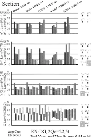
The statistical methods used in measurements to estimate maximum value of the samples of all meas-ured section can not be used in calculations as there are too few results. So the maximum of a assessment value out of all calculations are used as estimated value and compared to the limit value.
100 / lim
max ∗
=
The results of each wheel and of each evaluation section are shown.
Conclusion
Computer simulations promote designing a vehi-cle with good running performance and to prevent to fail in an assessment test. Simulation makes it possi-ble to study dynamic behaviour of the vehicle in de-tail. This opportunity should be used to find a good solution during the design process. In simulation it is easy to define any kind of track and to analyse the vehicle for all operation conditions.
A condensed form of assessment values is shown in Figure 11.
BIBLIOGRAPHY
1. Railway applications — Testing for the acceptance of running characteristics of railway vehicles – Testing of running behaviour and stationary tests, prEN14363; 2004.
2. Testing and acceptance of railway vehicles from the point of view dynamic behaviour, safety, track fa-tigue and running behaviour, UIC518, 2000. 3. Prevention of derailment of goods wagons on
dis-torted tracks, ERRI report B55, 1983; and Permissi-ble limit values for the Y and Q forces and derailment criteria; ERRI report C138, 1986.
4. Manual of AC-Rad-Schiene/Wheel-Rail RSPROF, RSGEO, RSANAPROF, RSRAIL, ArgeCare, 2004. 5. Bogies with steered or steering wheel sets; UIC
re-port C116, 1993.
6. COMPUTER SIMULATION OF RAIL VEHICLE DYNAMICS' Vehicle System Dynamics Vol. 30, Numbers 3-4, September 1998.
![Fig. 1. Coefficient of friction measured by UIC [3]](https://thumb-us.123doks.com/thumbv2/123dok_us/8024585.2125529/3.892.102.419.246.438/fig-coefficient-friction-measured-uic.webp)
![Fig. 3: Evaluation of measured rail deviations [4] Conicity, wheel rail profiles](https://thumb-us.123doks.com/thumbv2/123dok_us/8024585.2125529/4.892.473.786.388.539/fig-evaluation-measured-rail-deviations-conicity-wheel-profiles.webp)