An Energy-Efficient Communication Scheme in Wireless Cable Sensor Networks

(1)

An Energy-Efficient Communication Scheme in

Wireless Cable Sensor Networks

Xiao Chen

Department of Computer Science

Texas State University

San Marcos, TX 78666

Neil C. Rowe

Department of Computer Science

U. S. Naval Postgraduate School

Monterey, CA 93943

Abstract—Nowadays wireless sensor networks (WSNs) have attracted a great deal of study due to their low cost and wide-range applications. Most of the sensors used so far are point sensors which have a disc-shaped sensing region. In this paper, we study a new type of sensor: the fiber optic cable sensor. Unlike a traditional point sensor, this type of sensor has a rectangular sensing region with a processor installed on it to do processing and communication. Like wireless sensor networks with point sensors, energy-efficient communication is still an important issue in wireless sensor networks with cable sensors because of the need to efficiently use limited resources. To address the issue, we propose a Cable Mode Transition (CMT) algorithm, which determines the minimal number of active sensors to maintainK -coverage of a terrain as well as K-connectivity of the network. Specifically, it allocates periods of inactivity for cable sensors without affecting the coverage and connectivity requirements of the network based only on local information. Before presenting CMT, we first show the relationship between coverage and connectivity, then the eligibility algorithm permitting a cable sensor to decide whether to stay active. CMT calls the eligibility algorithm to schedule cables. Simulation results show that our scheme is efficient in saving energy and thus can prolong the lifetime of wireless cable sensor networks.

I. INTRODUCTION

Wireless sensor networks (WSNs) have attracted a great deal of study due to the low cost of sensors and their wide-range applications. WSNs provide a new class of computer systems and expand human ability to remotely interact with the physical world. Most of the sensors used so far are point sensors which have a disc-shaped sensing region.

Recently a new kind of sensor has become available for detecting seismic signals [4]. It uses a fiber optic cable which is actively queried by sending optical signals down it. Each cable has a processor on it to process data and communicate with other processors on other cables. The cable can be tens of kilometers long so one cable can provide extensive coverage. Comparing with the tradition point sensors, this kind of sensor has a long length of coverage area which makes it ideal for borders and roads. It will be helpful in detecting excavation behavior such as digging tunnels and planting explosive devices on the roads as well as providing a secure border with24/7surveillance for illegal immigrants. Like point sensors, wireless communication among cables is more flexible and convenient than wired communication in case the topology of the network changes due to cable

movement or failures. Also, as in the wireless point sensor networks, energy-efficient communication is very important in wireless cable sensor networks due to the limited power resource in cable processors and the inconvenience of charging their batteries frequently.

In this paper, we reduce energy consumption in wireless communication by proposingCMT: A Cable Mode Transition

algorithm, which determines the minimal number of active sensors to maintain K-coverage of a terrain as well as K -connectivity of the network. Here, K-coverage means that every point in the terrain is covered by at leastKcable sensors and K-connectivity means that if K −1 cable sensors fail the network is still connected. The CMT algorithm allocates periods of inactivity for cables without affecting the coverage and connectivity requirements of the network based only on local information. Specifically, we make the following contributions:

• This is the first study on energy-efficient communication for wireless cable sensor networks.

• Conditions have been found for coverage to imply con-nectivity using cable sensors.

• Our Cable Mode Transition algorithm is a distributed protocol that only requires local information.

• Simulations are conducted to verify the efficiency of the proposed scheme.

The rest of the paper is organized as follows: Section II is the preliminary, Section III formulates the problem, Section IV describes the energy-efficient communication scheme CMT in detail, Section V shows the simulation results, Section VI mentions the related work, and Section VII concludes the paper and points out the future direction.

II. PRELIMINARY

In this paper, the cable seismic sensors we use are different from traditional point sensors. They are different in both sensing and communication. The sensing region of a point sensorucan be modeled as a disc with a sensing rangesand its communication region can be modeled as a disc with a communication range r as shown in Fig. 1(a). For a cable sensor v deployed straight with length L in Fig. 1(b), its sensing rangeD is the maximum distance that can be sensed orthogonal to the cable, and its sensing region is a rectangle

(2)

u D D (b) A cable sensor s r R

(a) A traditional point sensor

L Rect(v)

v _p

Fig. 1. Traditional point sensor vs. cable sensor

denoted as Rect(v). That is, any object coming across this region can be detected by the cable. In some figures of this paper, the rectangular sensing region of a cable is represented by a shaded area. Actually, the sensing region of a cable should have rounded ends that are semicircles of radius D

since coverage extends past the ends of the cable for distance

D. Here we make the simplification based on the fact that there will be significant noise in the vicinity of the cable ends. The communication between cables is done by the processors on the cables. Each cable should have a processor to collect data and communicate with other processors on other cables. The processor pon cablev has a communication region of a disc with a communication range R and is represented by a dot. In this paper, we assume the terrain to be covered is a large

2-dimensional convex and a cable is always deployed straight because it is easy to prove that it covers the most sensing area if deployed in this way.

III. PROBLEMFORMULATION

We formulate the energy-efficient communication problem as follows: given a 2-dimensional convex terrain A, and a coverage degreeKspecified by the application, we must allow as many processors as possible to turn off most of the time and at the same time, enough processors must stay awake to guarantee that A is K-covered and the backbone formed by awakened processors isK-connected.

In this problem, there are two issues: coverage and con-nectivity. First we want to know if they are related. If one implies the other, then if we satisfy the stronger one, the other is also satisfied. Obviously connectivity does not imply coverage because if a network on a terrain is connected, it can happen that not every point in the terrain is covered by some sensor. On the other hand, if a terrain is fully covered by a sensor network, is the network connected? The following two theorems show the conditions for coverage to imply connectivity with1-coverage andK-coverage. The conditions are true regardless of the locations of processors on cables. Due to the limited space, the proofs of all theorems in this paper can be found in [2].

Theorem 1: For a set of cables having sensing rangeDand length L that 1-cover a 2-dimensional convex terrain A, the communication graph made by processors is connected if the communication range R≥2√L2+D2.

Theorem 2: A set of cables that K-cover a 2-dimensional convex terrain Aforms aK-connected communication graph

u v w Fig. 2. wis ineligible ifK= 1 ifR≥2√L2+D2. IV. THECMT ALGORITHM

From the above, we know that if a terrain is K-covered and if the communication range R ≥ 2√L2+D2, then the network isK-connected. In this section, we present the cable mode transition (CMT) algorithm to determine the minimal number of active cables to maintain K-coverage specified by the application as well as K-connectivity. The idea was inspired by [5]. The difference is that their approach applies to traditional point sensors with a disc-shaped sensing region and our approach applies to cable sensors with a rectangular sensing region.

A cable can be in one of the three modes with the en-ergy consumption from the highest to the lowest: ACTIVE, SNOOPY and SLEEP. In the ACTIVE mode, a cable actively senses and communicates with other processors on other cables; in the SNOOPY mode, each cable collects HELLO messages from its neighboring processors and checks its eligibility to determine its new mode; and in the SLEEP mode, a cable sleeps to save energy. The CMT algorithm describes the rules of cable mode transition to save energy. Before presenting CMT, we introduce the eligibility algorithm it calls whose role is to make each cable check its eligibility to stay active.

A. K-coverage eligibility algorithm

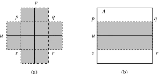
Each cable executes an eligibility algorithm to determine whether it is necessary to stay active. Given a requested coverage degree K, a cable v is ineligible to stay active if every location within its coverage region is alreadyK-covered by other active cables in its neighborhood. For example, in Fig. 2, cablesuandvare active and cablewis ineligible ifK= 1, but eligible ifK >1.

Before presenting the eligibility algorithm, we define the following concepts:

• The sensing region of cable v: contains all the pointsp

such that|pv|< D.

• An intersection point pof two cables uandv: denoted by p ∈ u∧v, is an intersection point of the sensing rectangles ofuandv.

• Anintersection pointpof a cable and terrainA: denoted by p ∈ u∧A, is an intersection point of the sensing rectangle of cableuand terrainA.

Note that the intersection points of two cables and between a cable and a terrain Aare different from regular definitions. Here they are formed by the sensing rectangles of cables, not

(3)

q p (a) (b) u u A s r s r p q v

Fig. 3. (a) The intersection points of cablesu andv(b) The intersection points between a cableuand a terrainA

Up D L D Vp v L p L u

Fig. 4. The largest distance of two neighboring cables

cables themselves. As shown in Fig. 3(a)(b), the intersection points of two cablesuandv and between cableuand terrain

A arep, q, r ands.

Also note that when deployed on a terrain, two cables may not be parallel or perpendicular to each other. They can intersect with any angle. But for convenience’s sake and without affecting the results, cables are drawn parallel or perpendicular to each other in Fig. 3.

Theorem 3: A convex terrain A is K-covered by a set of cables C if 1) there exist in terrain A intersection points between cables or between cables and A’s boundary; 2) all intersection points between any cables are at leastK-covered; and 3) all intersection points between any cable and A’s boundary are at leastK-covered.

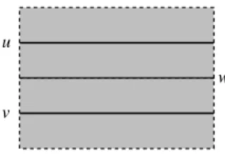
Theorem 3 converts the problem of finding the coverage degree of a terrain to the simpler problem of finding the coverage degrees of all the intersection points in the terrain. A cable is ineligible to stay active if all the intersection points inside its sensing rectangle are at least K-covered. To find all the intersection points inside its sensing rectangle, a cable v needs to know the locations of all the cables in its sensing neighbor set, SN(v). SN(v) should include all the active cables that are within the maximum distance between the processor on v and the processor on another cable that attaches tov. As shown in Fig. 4, that distance is the distance between processorvp onv andup on another cableu, which is (2L)2+ (2D)2 = 2√L2+D2. Cables can find their neighbors through exchanging Hello messages. If the actual communication rangeRused by a cable is greater or equal to

2√L2+D2, the Hello message from each cable only needs to include its own id and location. If R <2√L2+D2, a cable may not find all its neighbors through such Hello messages in one hop. Then, more cables will stay active because of its limited information. This is proved by the simulation in the next section. Also if R < 2√L2+D2, the network is not guaranteed to be connected as indicated by Theorem 2.

The resulting algorithm for a cable v to check whether it is eligible to stay active or not is shown in Fig. 5. Algorithm

Algorithm Eligibility: determine if a cable is eligible to stay active given a coverage degree K

1: /* find all intersection points within Rect(v)*/

2: _IP = {p | (p ∈ u∧w OR p ∈ u∧A) AND u, w ∈ SN(v)AND|pv|< D};

3: /* find all overlapping cables */

4: OC = {u| |uv|= 0}; 5: if |IP|= 0then 6: if |OC| ≥K then 7: return INELIGIBLE; 8: else 9: return ELIGIBLE; 10: end if 11: end if

12: foreach point p∈IP do

13: /* compute p’s coverage degree */

14: _cd(_p) =|{u|u∈_SN(_v) AND |pu|< D}|

15: if cd(p)< K then

16: return ELIGIBLE;

17: end if

18: end for

19: return INELIGIBLE;

Fig. 5. TheK-coverage eligibility algorithm

Eligibility has three parts: first, cablevfinds all the intersection points (of cables and between cables and terrain A) within its rectangular sensing region and puts these points into the intersection point set IP. Next, cable v tries to find out if there are anyoverlapping cableswhich are the cables happen to be placed in the same location as itself. If so, these cables are put into the overlapping cable set OC. If there is no intersection point withinv’s sensing rectangle and the number of overlapping cables|OC|is at leastK, cablevis ineligible. Otherwise, it is eligible. Finally, cable v calculates cd(p), the coverage degree of every intersection point p within its sensing region. If the coverage degree is less than K, cable

v is eligible; otherwise, it is not eligible. The computation complexity of the eligibility algorithm isO(N3) where N is the number of cables in the sensing neighbor set.

B. Cable mode transitions

Now the CMT algorithm is presented in Fig. 6. A cable can transit among SLEEP, ACTIVE and SNOOPY modes. Initially all cables are ACTIVE. If the terrain coverage goes over the required degree of the application, redundant cables will find themselves ineligible to stay active and go to the SLEEP mode until no more cables can be turned off without causing insufficient degree of coverage. If over time the failure of a cable makes the terrain coverage fall below the required degree, some cables will find themselves eligible and go to the ACTIVE mode. The times set by the join and withdraw timers are randomly generated to avoid collisions among multiple cables wanting to join or withdraw simultaneously.

(4)

Cable Mode Transition (CMT) Algorithm

1: If a cable is in the SLEEP mode and its sleep timer expires, it turns on, starts a snoopy timer and goes to the SNOOPY mode.

2: If a cable is in the SNOOPY mode and receives either HELLO, JOIN, or WITHDRAW message, it calls the eligibility algorithm (in Fig. 5) to see if it is eligible to stay active. If it is, it starts a join timer; else it goes to the SLEEP mode. After the join timer starts and if it becomes ineligible (e.g. because of a JOIN message from a communicating neighbor), it cancels the join timer. If the join timer expires, the cable broadcasts a ‘Join’ message and goes to the ACTIVE mode. If the snoopy timer expires, it starts a sleep timer and goes to the SLEEP mode.

3: If a cable is in the ACTIVE mode and receives a HELLO message, it updates its neighbor table and calls the eligibility algorithm (in Fig. 5) to see if it should remain active. If it should not, it starts a withdraw timer. Before the withdraw timer expires and if it becomes eligible (e.g. because of a WITHDRAW message from a communicating neighbor), it cancels the withdraw timer. If the withdraw timer expires, it broadcasts a ‘Withdraw’ message, starts a sleep timer and goes to the SLEEP mode.

Fig. 6. Cable mode transition algorithm

V. SIMULATIONS

In this section, we conduct simulations to evaluate our energy-efficient communication scheme. Our simulator is self-written because there are no available ones for cable sensors. We evaluate the effectiveness and properties of our scheme by itself due to the lack of others at this point.

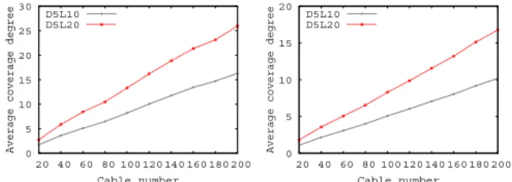
In the first simulation, we want to see the relationship between the number of cables deployed and the average coverage degree achieved. To measure coverage, we divide the entire terrain into 1×1 patches. The coverage degree of a patch is approximated by measuring the number of active cables that cover the center of the patch. We use terrains of

30×30and40×40. In each terrain, we try two kinds of cables: D5L10 (sensing range 5 and length10) and D5L20 (sensing range 5 and length20). Note that we do not have a unit for these data, which can make the simulations more adaptive to the real applications. What matters here is the relative size of the cables to the terrain. The cables are randomly deployed onto the terrain in all directions. We start from 20 cables to and go up to200cables with an increment of20in each step. The degree of each location is calculated and the final coverage degree of the terrain is the average of all the locations. Figs. 7(a)(b) show the results.

From the results, we can see that (1) in a larger terrain, the coverage is lower with the same number of cables; (2) in a terrain, with the increase of the number of cables, the coverage goes up; (3) with the same number of cables, the D5L20 cable has a higher coverage than the D5L10 cable

0 5 10 15 20 25 30 20 40 60 80 100 120 140 160 180 200

Average coverage degree

Cable number D5L10

D5L20

(a) Average coverage degree using D5L10 cables in a30×30terrain 0 5 10 15 20 20 40 60 80 100 120 140 160 180 200

Average coverage degree

Cable number D5L10

D5L20

(b) Average coverage degree using D5L20 cables in a40×40terrain Fig. 7. Average coverage degree achieved using different numbers of cables

0 20 40 60 80 100 140 160 180 200 220 240 Active cables Cable number 1-coverage 2-coverage 3-coverage

(a) Active D5L10 cables needed in a

30×30terrain for1,2,3-coverage

(b) Active D5L20 cables needed in a

(c) Active D5L10 cables needed in a

(d) Active D5L20 cables needed in a

40×40terrain for1,2,3-coverage Fig. 8. Active cables needed for1,2,and3-coverage

because it is longer and thus has a larger coverage region. In the second simulation, we want to find out how many cables are active out of all deployed to achieve coverage degrees 1,2, and3 using the CMT algorithm. Again we use the D5L10 and D5L20 cables and deploy them on two terrains

30×30 and 40×40. In terrain 30×30 using the D5L10 cables, we start from140cables because this is the number to guarantee1,2,and3-coverage for the whole terrain. Similarly in terrain30×30using D5L20 cables, the starting number is

120cables. And in terrain40×40, the starting cable numbers for D5L10 and D5L20 are 240 and 140 respectively for the same reason. The results are shown in Figs. 8(a)(b)(c)(d). From the results, we can see that (1) more cables need to be active to have higher coverage; (2) the number of active cables does not increase with the increase of cable numbers. That means, our scheme does not wake up more cables because the coverage goal has already been achieved.

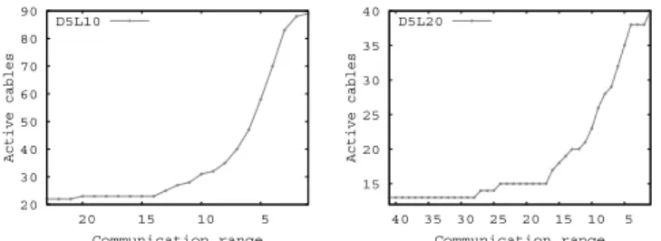
In the third simulation, we want to explore the effect of different communication ranges to the number of active cables using the CMT algorithm. We still deploy the D5L10 and D5L20 cables on the30×30and40×40terrains. To guarantee that a terrain is1-covered, we use different numbers of cables

(5)

20 30 40 50 60 70 80 5 10 15 20 Active cables Communication range D5L10

(a) Active D5L10 cables needed with different communication ranges in a

30×30terrain 15 20 25 30 35 5 10 15 20 25 30 35 40 Active cables Communication range D5L20

(b) Active D5L20 cables needed with different communication ranges in a

30×30terrain 40 60 80 100 120 140 160 180 200 220 5 10 15 20 Active cables Communication range D5L10

(c) Active D5L10 cables needed with different communication ranges in a

40×40terrain 25 30 35 40 45 50 5 10 15 20 25 30 35 40 Active cables Communication range D5L20

(d) Active D5L20 cables needed with different communication ranges in a

40×40terrain

Fig. 9. Active cables needed for different communication ranges

for each setting. For example, for terrain30×30with D5L10, we use90cables because this is the number to make sure that the terrain is 1-covered. For terrain 30×30with D5L20, we use40cables. For terrain40×40with D5L10 and D5L20, the number of cables used is 230 and 50 respectively. To make cases general, we put a processor on each cable in a random location. We start with a communication rangeRthat is greater or equal to2√L2+D2, then decrease it gradually. The results are shown in Figs. 9(a)(b)(c)(d).

From the results we can see that if the communication range is greater or equal to 2√L2+D2, many cables can be turned off because this is the range that they can fully detect their neighbors and find out if every location in their sensing region is1-covered by other active cables. For example, in the

30×30 terrain with the D5L10 cables, only 22 cables need to be active out of 90 cables deployed to1-cover the whole terrain. The saving is76%. Then we reduce the communication range. At the beginning, the number of active cables remains the same because the communication range is still greater than the distance between two processors on cables. Then with the further decrease of the communication range, each cable cannot fully detect all its neighbors even if they are there. From the limited neighbors that a cable can detect, it will more and more likely decide to stay awake because not all the locations within its sensing region can be covered by its detected neighbors. After a certain point, for example, in the 40 ×40 terrain with the D5L20 cables, when the communication range reduces to2or1, no cable can be turned off because each cable thinks it is the only one to cover the locations in its sensing region.

In summary, the simulation results show that the CMT scheme can make as many cables as possible to go to sleep

without affecting the connectivity of the network according to the required coverage degreeK from the application.

VI. RELATED WORK

In the literature, for point sensors, there are several papers working on saving power by determining a minimal number of active sensors to maintain coverage as well as connectivity. In terms of the relationship between coverage and connectivity, an important result was proved by Zhang and Hou [6], which states that if the communication range Rc is at least twice

the sensing range Rs, a complete coverage of a convex area

implies connectivity of the active sensors. Wang et al. [5] generalize the result in [6] by showing that, when the commu-nication rangeRcis at least twice the sensing rangeRs, aK -covered network will result in aK-connected network. Then the authors put forward the coverage configuration protocol (CCP) that can dynamically configure the network to provide different coverage degrees required by applications. Carle and Simplot [1] propose another mechanism for energy-efficient connected area coverage when all sensor nodes have the same sensing range and the communication range equals the sensing range. The goal of the algorithm is to use one of the existing protocols (e.g. Dai and Wu’s algorithm [3]) to select an area-dominating set of nodes of minimum cardinality, such that the selected set covers the given area.

VII. CONCLUSION AND FUTURE WORK

In this paper, we proposed a distributed algorithm called CMT to reduce communication energy consumption in a new type of sensor network: the fiber optic cable sensor network, by permitting processors take turns to go to sleep without affect-ing the coverage and connectivity of the network. Simulation results showed that our scheme is efficient in saving energy and can thus prolong the lifetime of the network. In the future, we will discuss point coverage and barrier coverage problems using cable sensor.

ACKNOWLEDGMENTS

This research was supported by NSF grant CBET 0729696. This work represents the opinions of the authors only and does not necessarily represent the views of the U.S. Government.

REFERENCES

[1] J. Carle, D. Simplot, “Energy efficient area monitoring by sensor networks,” IEEE Computer, vol. 37, No. 2, 2004, pp. 40-46. [2] X. Chen, N. C. Rowe, “Energy efficient communication of cable

sensors,” Technical report, Department of Computer Science, Texas State University, San Marcos, 2010.

[3] F. Dai, J. Wu, “Distributed dominant pruning in ad hoc wireless networks,”Proc. of IEEE International Conference on Commu-nications, 2003.

[4] N. Rowe, “Efficient deployment of fiber-optic cable seismic sensors,”Proc. of SIPE, April, 2010.

[5] X. R. Wang, G. L. Xing, Y. F. Zhang, C. Y. Lu, R. Pless and C. Gill, “Integrated coverage and connectivity configuration in wireless sensor networks,” Proc. of the 1st ACM SenSys, 2003, pp. 28-39.

[6] H. Zhang, J. C. Hou, “Maintaining sensing coverage and con-nectivity in large sensor networks,” Technical report UIUC, UIUCDCS-R-2003-2351, 2003.