EXTENSIONS OF NONPARAMETRIC
RANDOMIZATION-BASED ANALYSIS OF
COVARIANCE
Michael A. Hussey
A dissertation submitted to the faculty of the University of North Carolina at Chapel Hill in partial fulfillment of the requirements for the degree of Doctor of Public Health in the Department of Biostatistics.
Chapel Hill 2013
Approved by:
c
2013
Abstract
MICHAEL A. HUSSEY: Extensions of Nonparametric Randomization-Based Analysis of Covariance
(Under the direction of Gary G. Koch)
Nonparametric Randomization-Based Analysis of Covariance (Koch et. al. (1998))
provides covariate-adjusted estimates of treatment effects for randomized clinical
tri-als. It has application in the regulatory setting where analyses are specified a priori,
and any statistical assumptions of parametric methods are not verifiable until after
data collection. Using (1) a vector containing differences in means of outcomes and
differences in means of baseline covariables between the two randomized groups and
(2) an empirical covariance matrix for the vector, weighted least squares is applied to
force the difference in means of baseline covariables to zero (as expected with valid
ran-domization) to obtain covariate-adjusted estimates. The covariate-adjusted estimates
have a population-averaged interpretation and only require a valid randomization and
adequate sample size (for approximate normal distributions). Saville and Koch (2012)
have developed methodology combining cross-products of DFBETA residuals from a
treatment-only model with covariate information to obtain a covariance matrix for use
in the nonparametric covariate adjustment.
For this research, the methodology is extended to analysis of matched sets with a
di-chotomous outcome. In the 1:1 setting with randomization or M:1 setting, methods are
provided for obtaining an adjusted difference in proportions and an adjusted odds ratio,
including techniques for obtaining an exact p-value (for the difference). Application of
For larger strata, the methods of Saville and Koch are expanded to obtain stratified
covariate-adjusted log odds ratios (in the case of dichotomous outcomes) or stratified
covariate-adjusted log hazard ratios (in the case of time-to-event outcomes).
The methods of Saville and Koch are further developed for randomization to
mul-tiple treatment groups. Methodology is provided for creation of the appropriate
co-variance matrix to use in the nonparametric coco-variance adjustment, and a strategy for
accommodating a time-varying treatment effect is presented.
These methods avoid modeling assumptions for the covariates (e.g. proportional
hazards, functional form) while providing increased precision for the estimated
treat-ment effects. Their use is intended for primary analysis of a randomized clinical trial,
with supportive secondary parametric analyses having application to subgroup analyses
Acknowledgments
There are numerous people who have given me advice related to the content of this
dissertation and many who have given me their support throughout the process of its
creation. My utmost respect and gratitude goes to my advisor, Dr. Gary Koch. Your
insight and expertise helped this project happen, and I thank you for your patience
while I worked to understand the bigger research picture. I also thank you for generously
providing an academic home for me in the Biometric Consulting Laboratory during my
graduate career at UNC. The unique experience of being a student in the BCL is one
that has been transformative, and I will always look back on my time there with fond
memories. Most importantly, thank you for being a mentor in the truest sense of the
word. Your devotion to the next generation of biostatisticians is something I can only
hope to emulate in my career.
Additionally, I want to thank the members of my committee who have generously
given their time and experience to the research process: Dr. Amy Herring, Dr.
Anasta-sia Ivanova, Dr. Robert Millikan, Dr. John Preisser, Dr. Ben Saville, and Dr. Melissa
Troester. You gave me things to consider, and your contributions have improved the
final product significantly.
The experience of being a doctoral student is one that is often more about endurance
than it is about the difficulty of the work. It is in this regard that I have many people
to thank for their support. Thank you, Mom and Dad, for always being there when
very much, and I am so appreciative that you have supported me in whatever career
choices I’ve made. Many thanks to my family and friends, especially Michela Osborn,
Tania Osborn, Annie Green Howard, Margaret Polinkovsky, and Ashley Pinckney. You
provided balance to my academic life, and for this I will be always grateful (and sane).
Finally, I must thank the person who drew the short straw and got to be around
me every day while I finished this dissertation. Michael, thank you for being a trooper
through this process. Your support and motivation was essential when I wasn’t sure
Table of Contents
List of Tables . . . x
List of Figures . . . xii
1 Introduction and Literature Review . . . 1
1.1 Development of General Nonparametric Randomization-Based ANCOVA 2 1.2 Applications to Dichotomous, Ordinal, and Survival outcomes . . . 6
1.3 Stratification . . . 9
1.4 Other Applications . . . 10
1.5 Hybrid Methdology Using Diagnostics from Parametric Regression Models 12 1.6 A Note on Missing Data . . . 13
1.7 Summary of Research . . . 13
2 Analysis of Matched Studies with Dichotomous Outcomes using Non-parametric Randomization-Based Analysis of Covariance . . . 15
2.1 Introduction . . . 15
2.2 Methods . . . 17
2.2.1 All 1:1 Matched Sets with Randomization For Paired Difference . 17 2.2.2 Informative 1:1 Matched Sets for Odds Ratio . . . 20
2.2.3 M:1 Matched Sets with Randomization . . . 22
2.2.4 1:1 Matched Case-Control Studies . . . 25
2.3.1 Multi-Center 1:1 Clinical Trial Data for Improvement of a Skin
Con-dition . . . 26
2.3.2 Extension of Multi-Center Clinical Trial Data to 2:1 Setting . . . 30
2.3.3 1:1 Matched Case-Control Study of Vaccine Exposure and Influenza 35 2.4 Discussion . . . 38
3 Nonparametric Randomization-Based Covariate Adjustment for Strat-ified Analysis of Time-to-Event or Dichotomous Outcomes . . . 40
3.1 Introduction . . . 40
3.2 Methods . . . 43
3.2.1 Hybrid Methodology for Dichotomous Outcomes with Stratification 43 3.2.2 Hybrid Methodology for Time-to-Event Outcomes with Stratification 46 3.3 Examples . . . 48
3.3.1 Dichotomous Outcome: Neurologic Disorder Data . . . 48
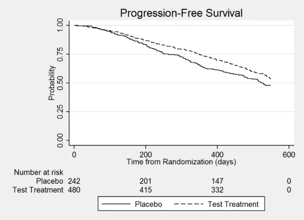
3.3.2 Time-to-Event Outcome: Neurologic Disorder Data . . . 50
3.3.3 Dichotomous Outcome: Osteoarthritis Data . . . 53
3.4 Discussion . . . 55
4 Covariate-adjusted Log Hazard Ratios using Cox Proportional Haz-ards Regression and Nonparametric Randomization-Based ANCOVA for More Than Two Treatments . . . 64
4.1 Introduction . . . 64
4.2 Methods . . . 66
4.2.1 Methodology for More than Two Treatment Groups and One Time-to-Event Outcome . . . 66
4.2.2 Estimation of Log Hazard Ratios for Time-Varying Treatment Effects with More than Two Treatment Groups . . . 70
4.3 Example . . . 72
4.3.2 Comparison of Four Treatment Groups with Time-Varying Treatment
Effects . . . 75
4.4 Discussion . . . 77
5 Summary and Future Research . . . 83
5.1 Summary . . . 83
5.2 Considerations and Limitations . . . 84
5.2.1 Missing Data . . . 84
5.2.2 Limitations . . . 85
5.3 Future Research . . . 85
Appendix A: Chapter 3 . . . 89
A.1 Specification of Covariance Matrix V˜f for Compound Vector in Stratified Analysis using Multivariate U-statistics . . . 89
A.1.1 Theoretical Specification . . . 89
A.1.2 Numerical Assessment . . . 93
A.2 Specification of Covariance Matrix V¯f for Compound Vector in Stratified Analysis through Transformation . . . 98
A.3 Numerical Examples for Different Covariance Specifications . . . 98
A.3.1 Dichotomous Outcome: Neurologic Disorder Data . . . 99
A.3.2 Time-to-Event Outcome: Neurologic Disorder Data . . . 100
A.3.3 Dichotomous Outcome: Osteoarthritis Data . . . 101
Appendix B: Chapter 4 . . . 106
B.1 Specification of Covariance Matrix for Compound Vector in NPANCOVA for Multiple Treatment Groups . . . 106
B.2 Covariance Matrices for Multivariate Time-to-Event Outcomes . . . 110
List of Tables
2.1 Matched Pairs Analysis of Multi-Center Clinical Trial Data from Example 2.3.1 . . . 28
2.2 Analysis of Multi-Center 2:1 and 1:2 Clinical Trial Data from Example 2.3.2 33
2.3 Analysis of 1:1 Matched Case-Control Study From Example 2.3.3 . . . . 37
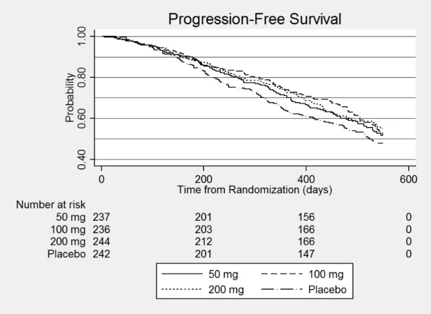
3.1 Progression by 12 Months for Patients with a Neurologic Disorder from Ex-ample 3.3.1 who Received Test Treatment (100 mg or 200 mg) or Placebo 49
3.2 Stratified Analysis for Dichotomized Outcome from Example 3.3.1 for Neu-rologic Disorder Data . . . 59
3.3 Strata Sizes and Number of Events for the 722 Patients Enrolled on the Placebo, 100 mg, or 200 mg Arms of the Neurologic Disorder Trial for Exam-ple 3.3.2 . . . 60
3.4 Stratified Analysis for Time-to-Event Outcome from Example 3.3.2 for Neu-rologic Disorder Data . . . 61
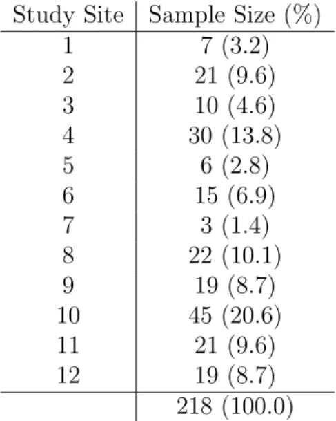
3.5 Strata Sizes for the 218 Patients with Data for Visits 1, 2, and 3 in the Osteoarthritis Randomized Crossover Trial for Example 3.3.3 . . . 62
3.6 Results from Example 3.3.3 for Osteoarthritis Data for the WOMAC Dichot-omized Outcome . . . 63
4.1 Results from Analysis on Four Treatment Groups with No Time-Varying Treatment . . . 80
4.2 Parameter Estimates for Interactions from Analysis with Time-Varying Treat-ment . . . 81
4.3 Results from Analysis with Time-Varying Treatment . . . 82
A.3.2 Stratified Analysis for Time-to-Event Outcome from Example 3.3.2 for Neu-rologic Disorder Data . . . 104
List of Figures
2.1 Frequencies of Success Outcomes for Treatment (T) * Placebo (P) for 1:2 and 2:1 Matched Sets for Data from Example 2.3.2 . . . 34
3.1 Kaplan-Meier Estimates of Progression-Free Survival for Neurologic Data from Example 3.3.2 . . . 51
Chapter 1
Introduction and Literature Review
Analysis of Covariance (ANCOVA) has long been used as a way of assessing the
relationship between a variable and an outcome measure in the presence of other
vari-ables. In an observational study, ANCOVA may be used when there is interest in
assessing the risk of disease associated with an exposure while adjusting for potential
confounders. Covariance adjustment is desired in this setting so as to reduce bias in
measuring the association between the exposure and risk of disease. In the randomized
clinical trial setting, ANCOVA may be used to assess the effect of a treatment on an
outcome measured after the treatment period while adjusting for a subject’s baseline
measurement. Covariance adjustment is desired in this setting so as to increase the
precision of the estimated treatment effect and increase statistical power of hypothesis
tests.
In general, covariance adjustment is desirable when analysis goals may involve (1)
the reduction of bias due to potential confounding in an observational study, (2) the
reduction of variance of an estimated treatment effect in a randomized clinical trial by
adjusting for highly predictive covariables, (3) correcting minor imbalances in the
dis-tributions of baseline variables between the treatment groups which may have occurred
treatment effects would otherwise be explained by other factors, and (5) through
inter-action, assessment of possible heterogeneity of treatment effects across groups defined
by other factors (Snedocor and Cochran, 1980).
For continuous outcomes, parametric ANCOVA methods such as linear regression
rely on the assumptions of independence of observations, homogeneity of error
vari-ances, correct functional form for covariates, and normality of the errors. For
dichoto-mous outcomes, logistic regression requires assumptions of independent binomial
distri-butions for the different subpopulations defined by cross-classification of the covariates
as well as correct functional forms for the covariates. For ordinal and time-to-event
outcomes, the proportional odds model and the Cox proportional hazards model
re-quire their respective assumptions of proportional odds and proportional hazards. In
the setting of a randomized clinical trial for an experimental treatment in support of
approval by a regulatory agency, all analyses on the primary endpoint must be specified
prior to data collection. The statistical assumptions related to parametric ANCOVA
methods are usually unverifiable a priori. This dilemma has led to interest in
apply-ing nonparametric randomization-based ANCOVA methods to data from randomized
clinical trials.
1.1
Development of General Nonparametric
Randomization-Based ANCOVA
Details for general methodology of nonparametric randomization-based ANCOVA
can be found in Koch, Amara, et. al. (Koch et al., 1982) as well as the appendix
of Koch, Tangen, et. al. (Koch et al., 1998). Let yik denote a univariate response
for patient k randomized to treatment i in a clinical trial. Here, k = 1, . . . , ni and
i= 1,2. Additionally, let xik = (xik1, . . . , xikP)0 denote the vector of P covariables for
mean of the covariates for patients on treatment i are given as ¯yi = n1i
Pni
k=1yik and
¯ xi = n1
i
Pni
k=1xik. Further, let f = (dy,d
0
x)0 wheredy = (¯y1−y¯2) and dx = (¯x1 −x¯2).
Thus f is a vector containing the difference in mean responses and the difference in means of covariables between the two treatment groups. In the case of a continuous
outcome, f exists as stated. In the case of other types outcomes, the dy may undergo
transformation or represent a difference in mean scores rather than a strict difference
in sample means.
A covariance matrix for f can be generated in one of two ways. Under a null hypothesis of no treatment effect, a randomization distribution can be derived under
an expectation that a patient’s response would be the same on either treatment. The
covariance matrix that is created, V0, has the form in (1.1).
V0 =
n n1n2(n−1)
n
X
k=1
(y∗k−y¯∗∗)2 (y∗k−y¯∗∗)(xk−x¯∗)0
(y∗k−y¯∗∗)(xk−x¯∗)0 (xk−x¯∗)(xk−x¯∗)0
(1.1)
Here,n=n1+n2,y∗kis the response under the null hypothesis for patientk(irrespective
of treatment assignment), ¯y∗∗ is the sample mean of all patients in the trial under the
null hypothesis, and ¯x∗ is the sample mean vector of covariates for all patients in the
trial. Since this covariance matrix is developed using a randomization distribution
based on a finite sample (i.e. those enrolled in the clinical trial), inference is confined
to the population of patients enrolled on the trial.
Alternatively, a covariance matrix can be created under the assumption that the
trial patients are a simple random sample from a larger population. Then the covariance
Vs can be defined as in (1.2):
Vs=
2 X
i=1
1 ni(ni−1)
ni
X
k=1
(yik−y¯i)2 (yik−y¯i)(xk−x¯i)0
(yik−y¯i)(xk−x¯i)0 (xk−x¯i)(xk−x¯i)0
This covariance matrix allows inference to the larger population from which the trial
pa-tients were sampled, thus allowing for population-based (i.e. unconditional) inferences
after covariate adjustment.
The linear modelf =Zbcan be fit using weighted least squares methodology, where Z = (100P)0 with 0P representing a zero vector of length P. This model specification
forces the difference in means of the covariables to zero, which is what is expected under
the assumption of a valid randomization. An estimator for b can then be obtained as
b= (Z0V−1Z)−1Z0V−1f whereV is either V0 orVs. An estimator for the variance of
b, Vb, can be obtained asVb = (Z0V−1Z)−1. This estimator corresponds to the exact
variance of the randomization distribution of b if V = V0. Otherwise, the estimator
corresponds to a consistent estimator of the variance of b if Vs is used.
Test statistics can be formed for the comparison of the two treatments using b
and its variance estimate Vb. When sample sizes are large enough for b to have an
approximate normal distribution (i.e. each treatment group has at least 15√P + 1
patients), Qb =b2/Vb will have an approximate chi-square distribution with 1 degree
of freedom (Koch et al., 1998). If Vs is used in the weighted least squares analysis,
large-sample confidence intervals for the treatment difference can be obtained through
the use of b and Vb. For small samples, an exact p-value for the test of the treatment
effect can be obtained (through a permutation test) when V0 is used as the covariance
matrix of f. Since the weighted least squares analysis using Z forces the difference in the means of the covariables between the two groups to zero, it may be of interest to
assess the extent of random imbalances in the covariables from randomization. Using
the V0 covariance matrix, one can create the test statistic Q0 = d0xV −1
xxdx which will
haveP degrees of freedom. Here, Vxx is the partition of V representing the covariance
matrix of the vector of mean differences in the covariables. A non-significant p-value
of a violation of the assumption of a valid randomization.
The methodology described above is a general framework for producing
nonpara-metric covariate-adjusted estimates of a treatment effect in a randomized clinical trial.
The main assumption is that there is a valid randomization to the treatment groups
so that the distributions of covariables are reasonably similar across the two treatment
groups. In the analysis described above, weighted least squares forces the difference
in means of the covariables between the two treatment groups to zero in line with
ex-pected differences under a valid randomization. With large enough sample sizes, the
covariate-adjusted estimates will have approximate normal distributions. The choice of
the covariance matrix used in the analysis will affect whether inference is restricted to
the study population or whether inference pertains to a large population from which
the study participants were randomly sampled.
There are some limitations to the methodology described above. Unlike standard
parametric regression approaches, estimates for the association between the covariables
and the response are not obtained. Usually this is not of concern, as the treatment
effect is generally the main association of interest in a randomized trial. Additionally,
as with any analysis of covariance, covariables should be chosen a priori so as to avoid
selection bias from choosing adjustment variables based on their relationship to the
outcome. Finally, the methodology presented here does not accommodate interactions
of covariates with treatment. However, estimation of treatment effects by levels of an
additional variable may be suitable in a supportive parametric analysis after statistical
significance of the treatment effect is established through the nonparametric analysis.
The estimated treatment effect obtained from the nonparametric ANCOVA here
should also be emphasized as representing a population-averaged treatment effect. In
parametric regression approaches, the estimated treatment effect is conditional in that it
in the unadjusted (treatment-only) parametric model would the estimated treatment
effect be population-averaged. Thus, the nonparametric ANCOVA methods tend to
be better suited to situations where interest is in an overall treatment effect rather
than one applying to certain subgroups of patients. It has been the recommendation of
authors (Koch et al., 1998),(LaVange, Durham and Koch, 2005) that the nonparametric
ANCOVA methods be reserved for analyzing the primary endpoint of a clinical trial
and that parametric regression models be supportive in secondary exploratory analyses
seeking to assess which subgroups may show greater benefit.
Given the flexibility of the above methodology to a variety of statistical outcomes,
much research has been conducted in recent years involving the application of the
nonparametric ANCOVA methods to different settings. The following sections detail
extensions of the methods to dichotomous, ordinal, and survival outcomes, as well as
discussing stratification and a hybrid methodology which uses parametric regression
diagnostics to obtain a covariance matrix for use in a nonparametric covariance
adjust-ment.
1.2
Applications to Dichotomous, Ordinal, and Survival
out-comes
The extension of nonparametric randomization-based ANCOVA to dichotomous
and ordinal outcomes is presented in Koch, Tangen, et. al. (Koch et al., 1998) and
Tangen and Koch (Tangen and Koch, 1999a). One of the main benefits of covariance
analysis is to achieve variance reduction in the estimated treatment effect. However,
due to the nonlinearity of the logit functions in logistic or proportional odds regression,
the estimated standard error of the treatment effect may increase after covariance
adjustment. This may cause some concern as to whether the parametric modeling
randomization-based ANCOVA methodology to a simple transformation of the outcome
measures.
Letyik be a dichotomous outcome where yik = 1 if patientk (k = 1, . . . , ni) shows a
particular response of interest on treatment i (i= 1,2) and yik = 0 if the patient does
not show that response. Then the sample mean of the responses for each treatment
is the proportion pi = ¯yi. The vector of covariables for adjustment follows the same
structure as in the general case. One can form a vectorfi for each treatment group as fi = (logit(pi),x¯0i)0, where logit(p) =loge(p/(1−p)). A difference vector d=f1−f2
can be created which includes the difference in the log odds of response between the
two treatments as well as differences in the means of the covariables between the two
treatment groups. The weighted least squares methodology can then be applied to
d with the model Z = (1 00P)0. The covariance matrix for d used in weighted least squares is usually Vs = V1+V2 since the vector d is a vector of differences between
the randomized groups. However, because a logit transformation was applied to the
response portion ofd, the covariance matrix would have the formD1V1D1+D2V2D2
where D1 and D2 are diagonal matrices of dimension P + 1 where the (1,1) element
of the matrices are ∂
∂p1loge(p1/(1−p1)) = 1
p1(1−p1) and
∂
∂p2loge(p2/(1−p2)) = 1
p2(1−p2),
respectively, and 1’s along the rest of the diagonal. V1 and V2 have the same form
as in (1.2) but for each treatment group separately. Chi-square tests for the treatment
effect as well as random imbalances in the covariates can be conducted as described in
the general methodology using the appropriate covariance structures.
In the case of the proportional odds model, one can expand the vectordto accommo-date the cumulative logits. For example, if the response variable had 4 categories (e.g.
extension of the covariance matrix which would consider (yik−y¯i)(yik−y¯i)0 instead of (yik−y¯i)2 and have the appropriate transformation via the relevant diagonal
matri-ces. Assessment of the treatment effect as well as random imbalances in the covariates
could proceed as previously described using Z = [Iu 0u,P]0 and Z = Iu+P,
respec-tively. Here,uis the number of cumulative logits,I corresponds to the identity matrix, and0u,P is au×P matrix of zeroes. A test of the proportional odds assumption could
proceed with the statistic Qw =b0C0(CVbC0)−1Cb where C = [−1(u−1) I(u−1)] and
1(u−1) is a vector of ones of length u−1. Qw is approximately chi-square with degrees
of freedom corresponding to rank(C).
Tangen and Koch also discuss the use of nonparametric ANCOVA methodology
for time-to-event data (Tangen and Koch, 1999b), (Tangen and Koch, 2001). One can
form the vectors f1 and f2 where the first entry corresponds to the average logrank (or Wilcoxon) score for treatments 1 and 2, respectively. Bivariate testing of both
types of scores could proceed with the first two entries of each vector corresponding
to the averages of each type of score. The covariance matrix used for the weighted
least squares portion would be based on randomization as in (1.1). Grouped survival
data can be accommodated as well where time intervals are exhaustive and mutually
exclusive. The response portion of the mean difference vector d consists of differences in cumulative survival rates in each of the relevant time intervals t = 1, . . . , T, where
the cumulative survival rates are based on products (up through the tth interval) of
conditional probabilities of surviving through intervaltgiven survival through the (t−
1) interval. The covariance of d is obtained through propagation of variances. A covariance matrix based on (1.2) is obtained from examining individual event and
at-risk information for the time intervals jointly. A series of matrix operations then
treatment effects, a test for random imbalances, and assessment of homogeneity of the
treatment effects across time intervals can all be obtained by appropriately specifying
Z matrices in a manner similar to the proportional odds analysis above; however, this approach does not provide a covariate-adjusted estimate of the hazard ratio.
1.3
Stratification
The nonparametric ANCOVA methods described thus far account for factors as
covariables. Extensions of the methodology to stratified studies have been presented
(Koch et al., 1998),(Tangen and Koch, 1999a),(Tangen and Koch, 1999b),(LaVange,
Durham and Koch, 2005). For randomized trials, a common stratification factor is
center in the context of a multi-center clinical trial. Other common stratification factors
could be geographic region or prognostic factors. For the purposes of nonparametric
randomization-based ANCOVA, two different approaches are recommended depending
on whether the strata are small (i.e. treatment group sizes within each stratum are
generally≤15) or large. In the case of small strata, the difference vector dh is created
for each of the q strata (h = 1, . . . , q). Covariance matrices Vs,h are also obtained
for each stratum. A weighted difference vector dw = Pqh=1whdh is obtained as well
as a weighted covariance matrix Vs,w = Pqh=1whVs,h. Here, the wh are usually the
Mantel-Haenszel weights (Mantel and Haenszel, 1959). Weighted least squares is then
applied using dw and Vs,w. When strata are large enough, weighted least squares can
be applied within each stratum and then the estimates bh and Vb,h can be combined
over strata using the Mantel-Haenszel weights. Associated tests for the treatment effect
1.4
Other Applications
Several other applications of nonparametric randomization-based ANCOVA have
been developed in recent years. Koch and Tangen extend the methodology to
non-inferiority clinical trials (Koch and Tangen, 1999). Consider a randomized trial with
test treatment (T), reference treatment (R), and placebo (P). Interest is in making
sure that both T and R are better than placebo and that T is also non-inferior to R.
The difference vectord can take the form of (dT P,u0T P, dRP,u0RP)0 where dT P and dRP
are the difference in mean responses between test and placebo as well as reference and
placebo, respectively. The uT P and uRP represent the differences in the means of the
covariables for test vs. placebo as well as reference vs. placebo. The differences in
the means of the covariables can be forced to zero through a weighted least squares
analysis which produces covariate-adjusted estimates of the differences between each
response and placebo jointly. Through an appropriate specification of Z, the ratio of (T-P) relative to (R-P) can be assessed, and Fieller’s formula (Fieller, 1954) can be
used to obtain a confidence interval for this ratio.
Kawaguchi, Koch, and Wang extend the methodology to the case where stratified
multivariate Mann-Whitney estimators are used to compare two treatments with
re-spect to any number of finite ordinal responses (Kawaguchi, Koch and Wang, 2011).
Here, the elements of vector f include the stratification-adjusted Mann-Whitney esti-mators for each of the responses as well as ratios comparing the two treatment groups
with respect to stratification-adjusted estimators of covariable means. A consistent
co-variance matrix for f can be obtained through propagation of variance and then used in the usual weighted least squares analysis to obtain covariate-adjusted estimates of
the treatment effect.
Saville, LaVange, and Koch extend the methodology to the estimation of incidence
use example data from a clinical trial for COPD where pulmonary exacerbations were
recorded as the events of interest. Considering six 6-month time intervals (3 years
of potential follow-up), the elements of the vector fhik are the counts of exacerba-tions, the time at risk, and the covariable values for individualk on treatment i in the
hth stratum during the J time intervals. A subsequent covariance matrix Vhi can be
formed for ¯fhi = Pni
k=1(fhik/ni). Weighted estimates of the ¯fhi and the Vhi can be
formed. From these, a compound difference vector d can be formed which contains the stratification-adjusted, log incidence density ratios comparing the two treatments
in each of the J time intervals as well as the stratification-adjusted differences in the
means of the P covariables. Weighted least squares can then be applied to dto obtain covariate-adjusted estimates of the log incidence density ratios. Subsequent hypothesis
tests and confidence intervals can be formed, including the test to check for random
imbalances in the covariates between the treatment groups. While the procedure just
described applies an order of stratification, estimation of log incidence density ratios,
and covariate adjustment, the ordering of these three steps can be changed depending
on the number of time intervals or the size of the strata. If the number of time intervals
is small, the covariate adjustment can occur prior to estimation of the log incidence
density ratios. In the event of large strata, estimation of log incidence density ratios and
covariate adjustment can occur within strata before the covariate-adjusted estimates
are combined across the strata using some form of weighting.
A similar approach was used to estimate covariate-adjusted log hazard ratios for
multiple time intervals as in Moodie, Saville, Koch, and Tangen (Moodie et al., 2011).
Elements of the vector fik for the kth patient on the ith treatment consist of J terms which assess survival of the time intervals and J terms which assess whether the
pa-tient was at risk in the J pre-specified time intervals under study. This vector also
each treatment fi can be formed, and an associated covariance matrix can be con-structed. Through the propagation of variance, a vector d is formed which represents the difference between the treatment groups with respect to log hazard ratios and the
means of the covariables. Weighted least squares then usesdand its covariance matrix Vd to obtain covariate-adjusted estimates of the log hazard ratios for theJ time
inter-vals. As in the general case, hypothesis tests for homogeneity of the log hazard ratios
from the J time intervals can be conducted along with a test of random imbalance in
the covariates between the two treatment groups.
1.5
Hybrid Methdology Using Diagnostics from Parametric
Regression Models
A common semiparametric approach to estimating a hazard ratio in the presence of
covariables is the Cox proportional hazards model for time-to-event data (Cox, 1972).
Saville and Koch proposed a covariate-adjusted log hazard ratio obtained via
nonpara-metric randomization-based ANCOVA which is closer to that of the Cox model than
what was described in Moodie et. al. (Moodie et al., 2011) (Saville and Koch, 2013).
Marginal Cox proportional hazards models containing a treatment indicator are fit for
each of K events. The K DFBETAs from these models are obtained for individuals
in each of the two treatment groups. The DFBETA for patient j (j = 1, . . . , ni) and
event k (k = 1, . . . , K) represents the approximate change to the kth estimated log
hazard ratio when the jth patient is omitted. Weiet. al. showed that an approximate
covariance matrix for the estimated log hazard ratios ˆβ,Vβˆ, can be obtained by taking
the sum of the cross-products of the DFBETAs (Wei, Lin and Weissfeld, 1989). If
the elements of the difference vector d are the estimated log hazard ratios ˆβ and the differences in means of the covariables (¯x1−x¯2), the associated covariance matrix Vd
is the estimated covariance matrix for (¯x1−x¯2) and Vβ,ˆx¯1 −Vβ,ˆx¯2 is the estimated
covariance of ˆβ with (¯x1 −x¯2). Here, Vβ,ˆx¯i is the estimated covariance matrix for ˆβ
and ¯xi for theith treatment group. Weighted least squares can then be applied usingd
and Vd via the model Z = [IK 0KP]0 to obtain covariate-adjusted log hazard ratios.
Tests of homogeneity across the K log hazard ratios and random imbalance of
covari-ables between the two treatment groups can be conducted per other specifications of
Z. While this hybrid procedure is not thought to be fully nonparametric since it makes use of a treatment-only Cox model, the p-value from the Cox model is comparable to
the nonparametric logrank test (Saville and Koch, 2013). The assumption of
propor-tional hazards for the covariates is avoided since covariate adjustment is made via the
nonparametric methodology.
1.6
A Note on Missing Data
The general nonparametric randomization-based ANCOVA methodology relies on
the assumption that the distributions of the covariables between the two treatment
groups are comparable as a consequence of a valid randomization. Exclusions of patients
for protocol violations or missingness on a covariate could potentially induce imbalance
in the covariate distribution between the two groups (Koch et al., 1998). However, the
methods would be applicable for any sort of valid multiple imputation strategy. For the
methodology in Kawaguchi, Koch, and Wang, missing data could be accommodated
when using the Mann-Whitney estimators, although a mechanism of missing completely
at random (MCAR) is assumed (Kawaguchi, Koch and Wang, 2011).
1.7
Summary of Research
The following chapters outline applications of nonparametric ANCOVA
sets data with dichotomous outcomes. Nonparametric methodology is introduced for
obtaining covariate-adjusted estimates of a treatment effect for 1:1 and M:1
random-ized studies as well as for 1:1 non-randomrandom-ized matched case-control studies. Such
applications are intended for matched pairs data (as an alternative to the unadjusted
McNemar’s analysis or conditional logistic regression) or when the size of the matched
set is ≤6. Chapter 3 outlines a hybrid methodology (like that in Section 1.5) for
con-ditional likelihoods (as in concon-ditional logistic regression) or partial likelihoods (as in
proportional hazards regression) in the presence of stratification. A treatment-only
regression model is fit, and the sum of the squared DFBETA residuals estimates the
covariance of the treatment effect which can then be used in a weighted least squares
analysis to provide covariate adjustment. Chapter 4 extends the hybrid methodology
to more than two treatment groups for time-to-event data as explored in Saville and
Chapter 2
Analysis of Matched Studies with
Dichotomous Outcomes using
Nonparametric
Randomization-Based Analysis of
Covariance
2.1
Introduction
Matching may arise in clinical trials where the objective is to establish superiority
of a new treatment to a control (which may or may not be placebo). These studies may
range from a multi-center clinical trial (where subjects in the same randomization block
or from the same site form a matched set) to studies in dermatology, opthalmology,
or dentistry (where an individual’s arms/legs, eyes, or sections of the mouth form a
matched set). Matching allows for eliminating variability in the outcome among the
matched sets, thus making it a useful technique when designing a clinical study. In
the case of matched pairs for a dichotomous outcome, McNemar’s test and its related
odds ratio can be used to assess whether the subjects are more likely to experience
success (vs. failure) on a new treatment than they are on the control (McNemar,
analysis of a binary outcome where data are from matched sets may proceed using
conditional logistic regression (Breslow and Day, 1980). In either type of analysis, log
odds ratios and their confidence intervals can be obtained to assess the effect of the
new treatment. Matched studies may also be of the form M:1, where M individuals
are randomized to treatment and one individual is randomized to control within a
matched set. In studies with blocked randomization, blocks formed as successive pairs,
triples, or groups of M + 1 patients may be matched on time of enrollment if it was
thought to be a prognostic factor. Retrospective case-control studies may also exhibit
M:1 matching, where M controls are matched to one case on variables which may be
thought to confound the relationship between an exposure variable and the odds of
being a case. For most practical purposes, M ranges between two and four subjects
(Stokes, Davis and Koch, 2012).
The NPANCOVA methodology is useful for providing covariate-adjusted estimates
of treatment effects for data from matched studies when assumptions of other methods
are not verifiable. In studies with randomization, a valid randomization is assumed so
that the differences in covariate means between the randomized groups are expected to
be zero. In the case of the observational matched case-control study (without
random-ization), the NPANCOVA methodology may be applicable provided that the exposed
and not exposed subjects within the informative matched sets have similar distributions
of other covariables across the matched sets if the matching is successful. This
chap-ter presents extensions of the NPANCOVA methodology to randomized studies with
1:1 orM:1 matching as well as an observational case-control study with 1:1 matching.
Examples presented include a randomized clinical trial with 1:1 matching, a
random-ized clinical trial with 2:1 matching, and a retrospective case-control study with 1:1
matching. Discussion of the advantages and limitations of the methodology follows the
2.2
Methods
2.2.1
All 1:1 Matched Sets with Randomization For Paired
Difference
Letyhi= 1 denote a success on theith treatment (i= 1,2) for pair h(h= 1, . . . , q),
and letyhi = 0 denote a failure. Additionally, letxhibe theP×1 vector ofP covariates
corresponding to the ith treatment for pair h. Within each of the respective pairs, the
two treatments have independent random allocation with equal probabilities of 0.5. A
vector of the differences in binary outcomes for the two treatments can be formed as
dh = (yh1−yh2). The possible values for dh are as follows:
dh =yh1−yh2 =
1 if yh1 = 1, yh2 = 0
0 if yh1 =yh2
−1 if yh1 = 0, yh2 = 1
Withuh = (xh1−xh2) denoting the difference between treatments for the covariables
xhiwithin a pair, a vectorfh = (dh,u0h)
0 can be formed for each pairh. The respective
fhare statistically independent on the basis of (1) the respective pairs being comparable to a random sample from a relevant target population and (2) the independent random
allocation of the two treatments within corresponding pairs. The mean vector f¯ = ( ¯d,u¯0)0 = 1qPq
h=1fh can be formed with an unbiased estimate for its covariance matrix
Vf¯ as shown in (2.1). Here, ¯d represents the unadjusted difference in proportions of
success between the treatments.
Vf¯=
1 q(q−1)
q
X
h=1
(fh−f¯)(fh−f¯)0 =
vd¯ V0d,¯¯u
Vd,¯¯u Vu¯
A covariate-adjusted estimate of the difference in proportions of successes on the
treat-ments can then be obtained using weighted least squares methodology by forcing the
difference in means for the covariables to zero. With adjustment for P covariables,
the model Z = (1 00P)0 can be fit to f¯, where 0P is a zero vector of length P. The
covariate-adjusted estimate b for the difference in proportions is given in (2.2).
b = (Z0V−f¯1Z)−1Z0V−f¯1f¯ = ( ¯d−V0d,¯¯uV−u¯1u)¯
=
q
X
h=1
(dh−V0d,¯¯uV−u¯1uh)/q
(2.2)
A consistent estimator for the variance ofb isVb in (2.3).
Vb = (Z0Vf¯−1Z)−1
= (vd¯−V0d,¯¯uV−u¯1Vd,¯¯u)
=
q
X
h=1
(dh−d)¯ −V0d,¯¯uV−u¯1(uh−u)¯
2
/q(q−1)
(2.3)
wherevd¯,Vd,¯¯u, andVu¯ are the sub-matrices ofVf¯that correspond to the variance of
¯
d, the covariance vector of ¯dwith u, and the covariance matrix of¯ u, respectively. The¯ estimatorb has an approximate normal distribution when the number of matched pairs
qis sufficiently large such thatf¯has an approximately multivariate normal distribution. Where n1 and n−1 represent the number of pairs with dh = 1 and the number of pairs
with dh = −1, min(n1, n−1)/(P + 1) should be ≥ 8 and, ideally, ≥ 10. It follows
that the statistic b2/V
b has an asymptotic chi-squared distribution with one degree of
freedom. A 100∗(1−α)% confidence interval for bmay be obtained as b±z1−α/2∗
√
Vb
wherez1−α/2 is the 100∗(1−α/2)th percentile of a standard normal distribution. When
degrees of freedom (where q0 is the number of pairs with dh = 0) would improve the
approximate basis of this confidence interval.
Under the null hypothesis of no treatment difference whereby each individual in a
pair has the same response regardless of treatment assignment, the exact distribution
for f¯has 2(q−q0) possible realizations, and the corresponding exact covariance matrix
Vf ,¯0 has the form in (2.4).
Vf ,¯0 =
1 q2
q
X
h=1
fhf0h
=
vd¯,0 V0d,¯u,¯0
Vd,¯¯u,0 Vu,¯0
(2.4)
One then obtains the estimateb0 = (Z0V−f ,¯10Z)−1Z 0
V−f ,¯10f¯, an estimator of its variance Vb,0 = (Z0Vf ,¯0−1Z)−1, and Qb,0 = b20/Vb,0 for each of N re-randomizations of the
treatment assignment. The proportion of the N re-randomizations with Qb,0 greater
than or equal to the observed Qb,0 would be the essentially exact p-value. Due to
computational feasibility, choosing N to be sufficiently large for appropriate precision
(e.g.,N = 100,000) may be a necessary Monte Carlo alternative to computing Qb,0 for
all 2q possible treatment assignments so that the standard error of p is about 0.0005
for one-sided p-values that are near or below 0.025.
Since Vf ,¯0 is constant for all 2q possible treatment assignments, one could compare
eachb0 from theN re-randomizations to the observedb0 instead of usingQb,0 to obtain
the exact p-value; the result will be identical. The exact analysis can be conducted
using a procedure such as PROC MULTTEST in SAS software (SAS Institute, Cary,
NC). However, it is important to note that when using the variance Vf ,¯0 in (2.4), a
trade-off is that the formal inference is restricted to the randomized study population,
Vf¯ in (2.1) which assumes generalizability through pairs being like a random sample
of pairs from a corresponding population.
This methodology relies upon the assumption of a valid randomization, under which
no differences between the means of the covariables are expected between the two
treatment groups. Random imbalances in these means between the two groups can be
assessed with the statistic
Qu¯ = (f¯−Zb)0Vf¯−1(f¯−Zb) (2.5)
For sufficiently large q, this statistic approximately has the chi-squared distribution
with P degrees of freedom, and its counterpart Qu¯,0 with b0 and Vf ,¯0 replacing b and
Vf¯can have exact assessment.
2.2.2
Informative 1:1 Matched Sets for Odds Ratio
If the assumption of similar covariate distributions in the treatment groups remains
applicable when non-informative pairs with dh = 0 are removed from the analysis,
other analysis approaches may be justifiable. Considerah,I for informative pairs, where
ah,I = 1 if Treatment 1 is a success and Treatment 2 is a failure and ah,I = 0 if
Treatment 1 is a failure and Treatment 2 is a success. Also, ah,I is considered missing
when the same outcome is observed for Treatment 1 and Treatment 2 within a pair,
and such non-informative pairshwith missingah,I are omitted from the analysis. With
zh,I = (ah,I,u0h,I) 0,z¯
I = (¯aI,u¯0I) 0 = 1
q0
Pq0
h=1zh,I, andVz¯I formed in a similar manner as
Vf¯in (2.1), the modelZ = (100P)0 can be fit toz¯I. Here, ¯aI represents the proportion
of pairs (amongq0 = (q−q0) informative pairs) with success on Treatment 1 and failure
on Treatment 2. An estimatebI = (Z0V−z¯I1Z)
−1Z0
V−z¯1
Iz¯I can be obtained via weighted
least squares with consistent variance estimator VbI = (Z
0
Vz¯I
−1
matched pairs odds ratio for the treatment effect is bI/(1−bI), with 100∗(1− α)%
confidence interval (bI,L/(1−bI,L), bI,U/(1−bI,U)) where bI,L =bI−z1−α/2∗ p
VbI and
bI,U =bI+z1−α/2∗ p
VbI.
Analysis may also proceed on dh,I for the informative pairs where dh,I = 1 if
Treat-ment 1 is a success and TreatTreat-ment 2 is a failure, and dh,I = −1 if Treatment 1 is a
failure and Treatment 2 is a success. Then ¯dIrepresents the difference in the proportion
of pairs with Success/Failure and the proportion of pairs with Failure/Success. With
a covariate-adjusted counterpart b∗I of the difference in proportions ¯dI and variance
estimator Vb∗
I using the dh,I, the matched pairs odds ratio is (b
∗
I + 1)/(1−b∗I) with
100∗(1−α)% confidence interval ((b∗I,L+ 1)/(1−bI,L∗ ),(b∗I,U + 1)/(1−b∗I,U)). Exact
analysis can proceed in this setting as previously described using the variance under
the null hypothesis in (2.6) wherefh,I = (dh,I,u0h,I) 0.
Vf¯I,0 =
1
(q0)2 q0
X
h=1
fh,If0h,I (2.6)
Alternatively, one can include all the pairs in the analysis by forming ah1 and ah2,
where ah1 = 1 if dh = 1 (0 else), and ah2 = 1 if dh = −1 (0 else). The vector
gh = (ah1, ah2,u0h)
0 can be created, and the associated mean vector g¯ = (¯a
1,¯a2,u¯0)0
and estimated covariance matrix Vg¯ can be formed in ways comparable to f¯and Vf¯.
A transformation (via Taylor series linearization) may then be applied such that the
modelZ = (1 00P)0 can be fit to ˜¯g= (loge(¯a1/¯a2),u¯0)0 using the transformed covariance
matrix V˜¯g =AVg¯A0, where
A=
1 ¯
a1
−1 ¯
a2 01×P
0P×1 0P×1 IP×P
˜b = (Z0
V−g˜¯1Z)−1Z0V−g˜¯1g˜¯ represents the adjusted estimate of the log of the matched pairs odds ratio and a consistent estimator for the variance of ˜bisV˜b = (Z0V˜¯g
−1
Z)−1. A large-sample 100∗(1−α)% confidence interval can be obtained for the log odds ratio as
˜b±z1−α/2∗p
V˜b. This approach retains the covariate information from non-informative
pairs so that similar covariate distributions in the treatment groups holds on the basis
of a valid randomization.
An alternative to Taylor series linearization for obtaining a confidence interval for
the odds ratio is Fieller’s theorem (Fieller, 1954). Since the matched pairs odds ratio
can be expressed as the ratio of two means, ¯a1/¯a2, this approach is applicable. Using
the vectorg¯and its covariance matrixV¯g, one obtains the covariate-adjusted estimates
˜b = (˜b1,˜b2)0 and its associated covariance matrix V ˜
b through weighted least squares.
One then forms the adjusted matched pairs odds ratio as ˜b1/˜b2, and the confidence
limits are the solutions xof a quadratic equationax2+bx+c= 0 wherea, b, and care
as follows:
a= ˜b22−z12−α/2∗(v˜b2)
b= 2∗[z21−α/2∗(v˜b1,˜b2)−
˜b1∗˜b2]
c= ˜b21−z12−α/2∗(v˜b1)
(2.7)
Here, v˜b2 and v˜b1 are estimated variances of ˜b2 and ˜b1, respectively, and v˜b1,˜b2 is their
estimated covariance obtained from V˜b. The quantity z12−α/2 = 3.84 in the case of a
95% confidence interval.
2.2.3
M
:1 Matched Sets with Randomization
The methodology in Section 2.2.1 may readily be extended toM:1 matched sets with
randomization. These types of sets may arise in randomized clinical trials where one
within the matched set. In practice, M usually ranges between two and four.
Assume, without loss of generality, that we haveM:1 matched sets whereM patients
are randomized to Treatment 1 and one patient is randomized to Treatment 2. Let
yhik = 1 denote a success for patient k on the ith treatment (i = 1,2) from set h
(h= 1, . . . , q), and let yhik = 0 denote a failure for patient k on the ith treatment from
set h. Here, k = 1, . . . , M if i = 1, and k = 1 if i = 2. Let ¯yh1· = M1 PMk=1yh1k be the
proportion of successes for the M patients on Treatment 1 in set h. Additionally, let
xhik be the vector of covariates corresponding to the ith treatment for patient k from
seth, and x¯h1·= M1 PMk=1xh1k is the mean vector of covariates for the M patients on
Treatment 1 from seth. A vector of the differences in outcomes for the two treatments
can be formed as dh = (¯yh1·−yh21). With uh = (x¯h1·−xh21) denoting the difference
between treatments for the means of the covariables within a set, a vectorfh = (dh,u0h) 0
can be formed for each seth. The mean vector f¯= ( ¯d,u¯0)0 = 1qPq
h=1fh can be formed
with an estimated covariance matrixVf¯similar to (2.1). A covariate-adjusted estimate
of the difference in proportions for the treatments can then be obtained in a similar
manner using weighted least squares methodology to obtain b as in (2.2) and Vb as
in (2.3). Random imbalances in the means of the covariables between the treatment
groups can be assessed using the statistic in (2.5).
Methodology for obtaining an exact p-value for the treatment comparison would
proceed in a similar manner to the methods described in Section 2.2.1 with the use of
Vf ,¯0 instead of Vf¯. Under the null hypothesis that the response of each of the M + 1
members of each set would be the same regardless of treatment assignment,Vf ,¯0 would
take the form in (2.7). As previously stated, exact inference would then be formally
restricted to the randomized study population.
Vf ,¯0 =
(M + 1) M2q2
q
X
h=1 2 X
i=1
nhi
X
k=1
Here, nh1 = M, nh2 = 1, and ghik = (yhik,x0hik)0 denotes the compound vector of
the response and covariates for the kth individual on the ith treatment from the hth
matched set. Additionally, the mean of this vector for the thehth matched set is given
asg¯h = M1+1P2i=1Pnhi
k=1ghik. The formula (2.7) takes into account the M + 1 possible
ways to assignM individuals to Treatment 1 and one individual to Treatment 2. When
M = 1, the formula reduces to the form in (2.4).
A covariate-adjusted odds ratio may also be obtained for the M:1 setting. The
procedure begins with an unadjusted estimate of the odds ratio such as the
Mantel-Haenszel estimate (Breslow and Day, 1980), (Mantel and Mantel-Haenszel, 1959) as in (2.8).
ˆ ψmh =
PM
m=0mnm,0
PM
m=0(M −m)nm,1
(2.8)
Here, nm,1 is the number of matched sets with m successes among the M subjects
on test treatment and one success on control, and nm,0 is the number of matched sets
with m successes on test treatment and zero successes on control. One could also
define ah1 = m if there are m successes on test treatment when there is a failure on
control (m = 0, . . . , M) for matched set h, and define ah1 = 0 if there is success on
control. Similarly, defineah2 =M−m if there arem successes on test treatment when
there is a success on control, and define ah2 = 0 if there is failure on control. Then
Pq
h=1ah1 equals the numerator of ˆψmh and
Pq
h=1ah2 equals the denominator of ˆψmh.
A vector gh = (ah1, ah2,u0h)
0 can be formed. Its mean vector ¯g and covariance matrix
V¯g are formed as in Section 2.2.1. Covariate adjustment may then proceed through the
application of weighted least squares to the transformed vectorg˜¯= (loge(¯a1/¯a2),u¯0)0 =
(loge( ˆψmh),u¯0)0 using its transformed covariance matrix. Construction of a large-sample
confidence interval for the log odds ratio could proceed based on the covariate-adjusted
estimate ˜band its estimated variancev˜b as in Section 2.2.1. Alternatively, the
weighted least squares using g¯and V¯g, and Fieller’s theorem is then applied to create
a confidence interval for the ratio ˜b1/˜b2.
2.2.4
1:1 Matched Case-Control Studies
Matched sets often arise in non-randomized case-control studies where interest lies
in assessing the relationship between a dichotomous exposure (Yes/No) and case-control
status. The mechanism of NPANCOVA can be applied to a 1:1 matched case-control
study as follows: Define yh1 = 1 if the case from pair h was exposed and yh1 = 0 if
that case was not exposed. Similarly, define yh2 = 1 if the control from pair h was
exposed and yh2 = 0 if not exposed. Let xh1 be the covariates for a case, and let xh2
be the covariates for a control. It should be noted that in the case-control setting, the
difference in the means of covariables defined by case-control status is not likely zero
unless the covariables are not predictive of case-control status.
Consider dh = yh1(1−yh2)−yh2(1−yh1). Then dh = 1 if the case from pair h
is exposed and the control from pair h is not, dh = 0 if the case and control have
the same exposure status, and dh = −1 if the control is exposed and the case is not.
Further define ch = yh1(1−yh2)(xh1 − xh2) + yh2(1− yh1)(xh2 − xh1). Note that
ch =dh(xh1−xh2). Thus, when the case is exposed and the control is not exposed in
pairh,ch represents the difference in the covariables of exposed and unexposed. When
the control is exposed and the case is not exposed in pairh,ch represents the difference
in the covariables of exposed and unexposed as well.
The NPANCOVA methodology may then be applied to a vector fh = (dh,c0h) 0 as
in the setting with randomization. Use of ch ensures the difference in the means of
covariables will be defined by exposure status rather than case-control status, although
the analysis excludes sets where both the case and control within a pair are exposed
definition). The odds ratio and its confidence interval can be formed via the
methodol-ogy relating to the informative pairs analysis on thedh,I in Section 2.2.2, and pairs are
excluded when the dh = 0. The mean vector f¯I is formed as before and Vf¯I is created
as in (2.1). The covariate-adjusted estimate b∗I is formed as in (2.2) and its consistent
variance estimator Vb∗I is formed as in (2.3). It should be noted that while this odds
ratio is technically the exposure odds ratio, this quantity is algebraically equivalent
to the disease odds ratio of interest. Assessment of goodness-of-fit (in the sense of
comparable distributions of covariates for the exposure groups) may proceed using the
statistic in (2.5) using data for the informative pairs analysis.
2.3
Examples
2.3.1
Multi-Center 1:1 Clinical Trial Data for Improvement of
a Skin Condition
Researchers enrolled one pair of individuals from each of 79 randomly selected
clin-ics. For each pair, one individual was randomly chosen to receive the test treatment,
and another individual was randomly chosen to receive placebo. The initial grade of
a skin condition (coded 1-4 for mild to severe) was recorded for each patient. The
outcome of improvement in the skin condition was recorded as a 1 for improvement
and 0 for no improvement. A matched pairs analysis is appropriate for these data, with
adjustment for initial grade of the skin condition. Thirty-four (43%) pairs showed
im-provement for the patient receiving test treatment and no imim-provement for the patient
receiving placebo. Twenty (25%) pairs showed improvement for the placebo patient
but not the patient on test treatment. The remaining 25 (32%) pairs were concordant
(both members of a pair showed improvement or both showed no improvement). The
data are available in (Stokes, Davis and Koch, 2012).
in proportions of individuals with improvement on test (but not placebo) and placebo
(but not test) wasd= ((34/79)−(20/79)) = 0.1772 (S.E.=√vd=0.0909). With respect
to √vd,0 under the null hypothesis, the unadjusted McNemar’s test statistic d2/vd,0
had p=0.0567 from its approximate chi-squared distribution with d.f.=1; and its exact
counterpart from McNemar’s test was 0.0759 via the EXACT MCNEM option in SAS
PROC FREQ. When covariate adjustment was made, the adjusted estimate of the
difference in proportions was 0.1930 with an associated 13% reduction in the standard
error (S.E.=0.0791). The treatment effect was found to be statistically significant via
Qb,0 =b20/vb,0 with p=0.0181; the corresponding exact counterpart had p=0.0179 based
on N = 100,000 re-randomizations for the NPANCOVA analysis. The approximate
two-sided 95% confidence interval for the difference in proportions from NPANCOVA
was (0.0380, 0.3480). An approximation using thet-distribution with (q−q0−1−P) =
(79 −25 −1 −1) = 52 degrees of freeom was (0.0343, 0.3517). No evidence of a
random imbalance in initial skin condition between the two treatment groups was found
When only informative strata were considered in the analysis, the adjusted
pro-portion of individuals with a success on test treatment (and failure on placebo) was
0.6262. This was statistically different from 0.5 with a p-value of 0.0288. The odds of
success on test treatment (and failure on placebo) were (0.6262/0.3738)=1.6754 times
the odds of success on placebo (and failure on test). When considering the difference
in proportions for the informative pairs, the resulting odds ratio and p-value were
iden-tical, and the exact p-value was 0.0280. Among the informative strata, there was no
evidence of a random imbalance in initial skin condition between the two treatment
groups (Qu¯ = 0.0088, df=1, p=0.9251).
The unadjusted McNemar’s odds ratio was 34/20 = 1.7000, whereas when adjusting
for intial skin condition, conditional logistic regression produced an odds ratio of 2.0366,
and this estimate was statistically significant (p=0.0353). The NPANCOVA analysis
on all pairs produced an adjusted odds ratio (1.7842) similar to the McNemar’s odds
ratio, and a 13% reduction in the standard error for its logarithm (from the McNemar’s
S.E. of 0.2818) was observed (S.E.=0.2462). This resulted in a statistically significant
p-value for the treatment effect (p=0.0187). It should be noted that the estimated odds
ratio for NPANCOVA tends to be closer to the null of 1.0 than the conditional logistic
regression estimate because the NPANCOVA estimate is like a population-averaged
estimate relative to covariates for matched subjects, and the conditional logistic
regres-sion estimate has a subject-specific interpretation for matched patients with the same
initial skin condition.
The 95% large-sample confidence interval for the McNemar’s odds ratio was (0.9785,
2.9533), while a slightly more conservative interval using Fieller’s theorem (data not
shown) produced an interval of (0.9941, 3.1794). For the covariate-adjusted odds
theorem was (1.1198, 3.0913). While the large-sample intervals were based on
esti-mates where the log odds ratio was first created then underwent covariate adjustment,
the Fieller’s theorem intervals were based on creating a ratio of the covariate-adjusted
means. In the unadjusted case, the estimated matched pairs odds ratio was 1.7
re-gardless of method. For the adjusted case, the different approaches produced similar
estimated odds ratios (1.7842 for NPANCOVA, 1.7846 for ratio of adjusted means).
2.3.2
Extension of Multi-Center Clinical Trial Data to 2:1
Set-ting
To illustrate the application of the NPANCOVA methodology to a randomized
clinical trial with 2:1 matching, the data from Example 2.3.1 were re-examined. The
54 informative pairs and the 25 non-informative pairs were ordered separately by the
average baseline age for a pair. Starting with the smallest average baseline age, the
first non-informative pair was divided so that the patient on treatment was assigned
to treatment for the first informative pair, and the patient on placebo was assigned
to placebo for the second informative pair. The next non-informative pair on the
list was divided so that the patient on placebo was assigned to placebo for the third
informative pair, and the patient on treatment was assigned to treatment for the fourth
informative pair. This procedure continued (with the division of the 53rd informative
pair and deletion of the 54th informative pair) until 26 2:1 sets and 26 1:2 sets were
created. Since age had essentially no association with the response (within pairs), this
assignment was essentially random and kept all but one of the original pairs in the
analysis data set.
Since the data contain matched sets of different type (e.g. 2:1 and 1:2), a stratified
application of NPANCOVA was warranted (Koch et al., 1998). The vectors ¯d1 and u¯1
2.2.1. Separate f¯1 and f¯2 vectors and covariance matrices Vf¯1 and Vf¯2 were also
formed as appropriate. A weighted estimatef¯w = (q1f¯1+q2f¯2)/(q1+q2) and weighted
covariance matrix Vf¯w = (q21Vf¯1 +q22Vf¯2)/(q1+q2)2 were created, where q1 = 26 and
q2 = 26 were the numbers of 2:1 and 1:2 sets, respectively. Weighted least squares was
then applied tof¯wusingVf¯w to obtain an estimate adjusted for initial skin condition. If
the number of matched sets for each type of allocation was ≥50, covariate adjustment
could have been applied to the 2:1 sets and 1:2 sets separately before weighting the
estimates across type of matched set.
A stratified version of the methodology for the odds ratio can be applied in a similar
manner. For the 2:1 sets, the procedure for obtaining the estimate and its covariance
matrix is as described in Section 2.2.3. For the 1:2 sets, ah1 = 2,1, or 0 if 0,1, or 2
placebo successes were observed in set h when a test success was observed and is 0
if a test failure was observed, and ah2 = 0,1, or 2 if 0,1, or 2 placebo successes were
observed in set h when a failure on test was observed and is 0 if a test success was
observed. A vector g¯j = (¯a1j,a¯2j,u¯0j)0 was formed for each type of allocation so that
j = 1 for the 2:1 sets and j = 2 for the 1:2 sets. Corresponding covariance matrices
V¯gj (j = 1,2) can be formed through the expression in (2.1). A weighted vector
¯
gw = (¯a1w,a¯2w,u¯0w)
0 and its covariance matrix V ¯
gw are then formed as above. Then
the Mantel-Haenszel estimate of the log of the odds ratio for test vs. placebo would
be given as loge(¯a1w/¯a2w) and covariate adjustment could proceed via weighted least
squares with the vector g˜¯w = (loge(¯a1w/¯a2w),u¯0w)0, covariance matrixVg¯˜w =AV¯gwA
0
,
and model Z = (100P)0.
Results are presented in Table 2.2. The unadjusted difference in proportions
be-tween the test and placebo groups was 0.1923 (S.E.=0.1084). At the 0.05 level, this
result was not significantly different from zero with p=0.0761. However, with respect to
with this being identical to the Mantel-Haenszel p-value from SAS PROC FREQ. When
adjusting for initial skin condition, the difference in proportions for NPANCOVA using
the variance form in (2.1) weighted across the strata was 0.2087 (S.E.=0.0865). This
was statistically significant with a p-value of 0.0158. The assessment for random
imbal-ances in mean initial skin condition between the two treatment groups hadQu¯ = 0.0632
with df=1 and p=0.8015, indicating no evidence of an imbalanced randomization with