Differential Tracking through Sampling and
Linearizing the Local Appearance Manifold
Hua Yang
A dissertation submitted to the faculty of the University of North Carolina at Chapel Hill in partial fulfillment of the requirements for the degree of Doctor of Philosophy in the Department of Computer Science.
Chapel Hill 2008
Approved by:
Greg Welch, Advisor
Gary Bishop, Reader
Leonard McMillan, Reader
Marc Pollefeys, Reader
c °2008 Hua Yang
Abstract
Hua Yang: Differential Tracking through Sampling and Linearizing the Local Appearance Manifold.
(Under the direction of Greg Welch.)
Recovering motion information from input camera image sequences is a classic problem of computer vision. Conventional approaches estimate motion from either dense optical flow or sparse feature correspondences identified across successive image frames. Among other things, performance depends on the accuracy of the feature detection, which can be problematic in scenes that exhibit view-dependent geometric or photometric behaviors such as occlusion, semi-transparancy, specularity and curved reflections. Beyond feature measurements, researchers have also developed approaches that directly utilize appearance (intensity) measurements. Such appearance-based approaches eliminate the need for feature extraction and avoid the difficulty of identifying correspondences. However the simplicity of on-line processing of im-age features is usually traded for complexity in off-line modeling of the appearance function. Because the appearance function is typically very nonlinear, learning it usually requires an impractically large number of training samples.
I will present a novel appearance-based framework that can be used to estimate rigid motion in a manner that is computationally simple and does not require global modeling of the appearance function. The basic idea is as follows. An n-pixel image can be considered as a point in an n-dimensionalappearance space. When an object in the scene or the camera moves, the image point moves along a low-dimensional appearance manifold. While globally nonlinear, the appearance manifold can be locally linearized using a small number of nearby image samples. This linear approximation of the local appearance manifold defines a mapping between the images and the underlying motion parameters, allowing the motion estimation to be formulated as solving a linear system.
I will address three key issues related to motion estimation: how to acquire local appearance samples, how to derive a local linear approximation given appearance samples, and whether the linear approximation is sufficiently close to the real local appearance manifold. In addition I
Acknowledgments
I would like to express my sincere gratitude to my adviser Greg Welch. Throughout the years of my Ph.D. study, I have continuously benefit from his knowledge, his inspiration and his great efforts to explain things clearly and simply. His understanding, encouraging and personal guidance have made this long journey a pleasant one.
I would like to thank Marc Pollefeys for his insightful ideas that contribute to the basis of this dissertation. I am also very grateful to the other committee members: Gary Bishop, Leonard McMillan and Leandra Vicci. This dissertation could not have been finished without their invaluable suggestions and comments.
I am indebted to all the people who have helped my research from different perspectives. I would like to thank Jan-Michael Frahm for his valuable advice on several research projects. I wish to thank Adrian Ilie for his excellent camera calibration program that has been used in a number of experiments reported in this dissertation. I am grateful to Henry Fuchs and Andrei State for their guidance and support in my RA projects. I would like to express my appreciation to Herman Towles and John Thomas for their help in the hardware setup. I also thank Jingdan Zhang for the interesting discussion on a variety of research topics.
Lastly and most importantly, I would like to thank my wife Chen Jiang and my parents Jianhua Gu and Deben Yang. I would not have gone this far without their love and support. I dedicate this dissertation to my son, Michael Kai Yang, who has been cooperative during my disseratation writing.
Table of Contents
List of Tables . . . ix
List of Figures . . . x
List of Abbreviations . . . xii
1 Introduction . . . 1
1.1 Motion estimation . . . 1
1.2 Tracking as solving a reverse mapping . . . 2
1.3 Tracking through sampling and linearizing the local appearance manifold 5 1.4 Thesis statement and main contributions . . . 6
1.5 Thesis outline . . . 7
2 Related work . . . 8
2.1 Image measurements . . . 9
2.2 Feature-based motion estimation . . . 12
2.2.1 Model-based approaches . . . 12
2.2.2 Structure from motion approaches . . . 16
2.3 Flow-based motion estimation . . . 18
2.3.1 Flow estimation . . . 19
2.3.2 Motion estimation . . . 21
2.3.3 Direct methods . . . 22
2.4 Appearance-based motion estimation . . . 23
2.4.2 Image-based approaches . . . 25
2.5 Discussion . . . 28
3 Differential Camera Tracking . . . 31
3.1 Tracking by surfing the appearance manifold . . . 31
3.2 Linearizing the local appearance manifold . . . 33
3.3 Estimating incremental motion . . . 35
4 Sampling the local appearance manifold . . . 38
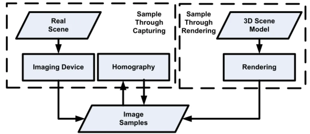
4.1 Sampling through capturing . . . 38
4.1.1 Differential camera cluster . . . 39
4.1.2 Inter-camera calibration . . . 40
4.2 Sampling through rendering . . . 44
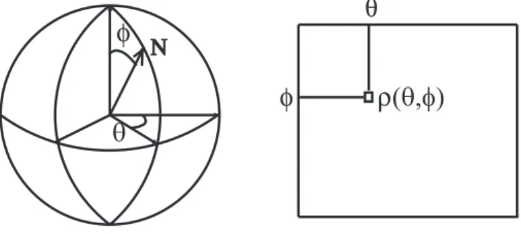
4.2.1 Illumination Normal Map . . . 44
4.2.2 Iterative estimation . . . 47
5 Analysis on sampling appearance manifolds . . . 52
5.1 Sampling the appearance signals . . . 53
5.2 Fourier analysis of the local appearance manifold . . . 54
5.2.1 Fourier analysis of the reference image . . . 55
5.2.2 Fourier analysis of X or Y translation . . . 56
5.2.3 Fourier analysis of Z translation . . . 58
5.2.4 Fourier analysis of rotation around X or Y axis . . . 61
5.2.5 Fourier analysis of rotation around Z axis . . . 63
5.2.6 Discussion . . . 66
5.2.7 Fourier analysis of the 8D appearance function . . . 67
5.3 Fourier analysis on general scenes . . . 69
5.3.1 Semitransparancy . . . 69
5.3.2 Occlusion . . . 70
5.3.3 Specular hightlights . . . 78
6 Motion Segmentation . . . 85
6.1 Related work . . . 85
6.2 Clustering motion subspaces . . . 87
6.2.1 Intensity trajectory matrix . . . 87
6.2.2 Motion subspaces . . . 89
6.2.3 Motion subspaces under directional illumination . . . 90
6.3 Motion segmentation by clustering local subspaces . . . 92
6.4 Acquiring local appearance samples . . . 95
7 Experiment results . . . 97
7.1 Differential camera tracking using online samples . . . 97
7.2 Differential object tracking using an off-line appearance model . . . 102
7.3 3D dense motion segmentation . . . 104
8 Conclusion and future work . . . 116
8.1 Summary of the thesis . . . 116
8.2 Future work . . . 119
Appendix A: Projective camera model . . . 124
Appendix B: Motion projection and image flow . . . 126
Appendix C: Kalman Filtering . . . 131
List of Tables
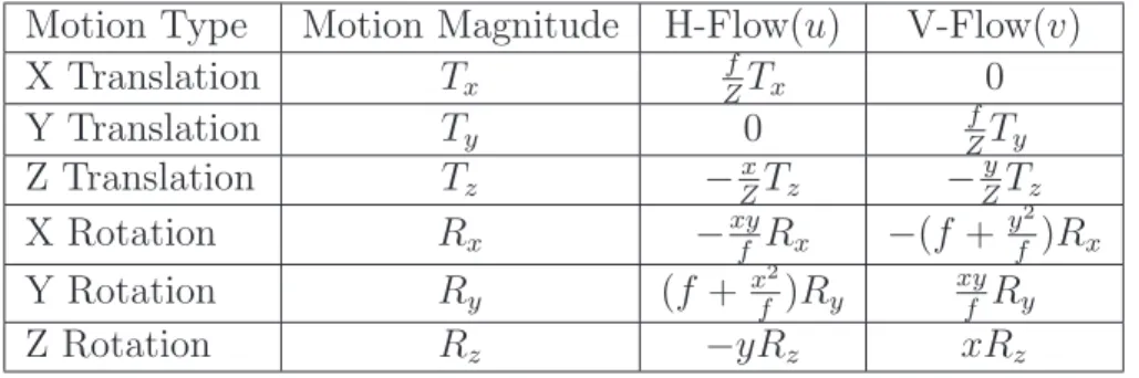
5.1 Optical flow of six 1D motions. . . 55
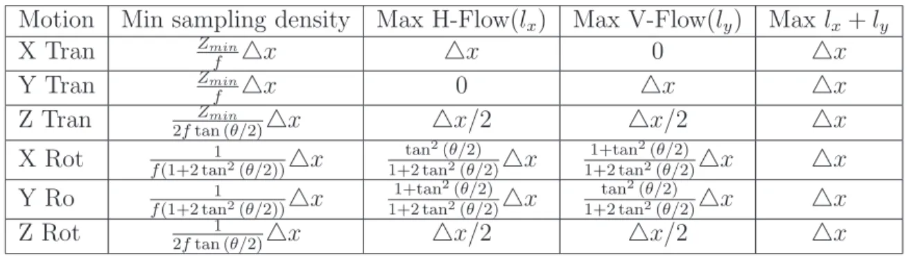
5.2 Minimum sampling density and maximum flow. . . 66
8.1 Optical flow of six 1D motion . . . 130
List of Figures
1.1 Motion estimation as solving a reverse mapping. . . 3
3.1 Appearance space and appearance manifold . . . 32
3.2 Manifold surfing . . . 34
4.1 Techniques for acquiring appearance samples. . . 38
4.2 A prototype differential camera cluster and illustrative images. . . 41
4.3 Illustration of illumination correction. . . 45
4.4 Spherical coordinate and INM. . . 46
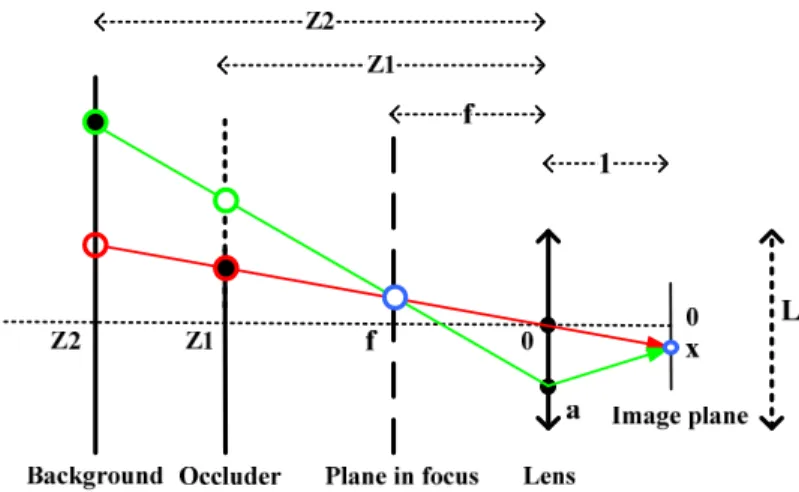
5.1 Illustration of occlusion observed by a thin-lens camera. . . 75
5.2 Illustration of specular reflection. . . 78
5.3 Fourier transform of the 2D cross-sections of the 3D appearance functions associated withX and Z translations. . . 83
5.4 Fourier transform of four 3D appearance functions associated with four 1D motions . . . 84
7.1 Tracking in a synthetic scene with a curved mirror. . . 99
7.2 Tracking a controlled camera motion. . . 100
7.3 Tracking a hand-held camera motion. . . 107
7.4 Tracking a hand-held camera cluster in a scene with semi-transparency. . 108
7.5 Tracking a hand-held camera with known ground-truth motion. . . 109
7.6 Illustration of the illumination correction process. . . 110
7.7 Tracking and INM estimation of a synthetic image sequence with varying illuminations. . . 111
7.9 Tracking of a real Lambertian object under directional lighting. . . 112
7.10 Texture refinement results on real data. . . 112
7.11 Motion segmentation and tracking results for a controlled sequence. . . . 113
7.12 Segmenting free-form rigid motions using a camera cluster. . . 114
7.13 Segmenting free-form rigid motions using a single camera. . . 114
7.14 Motion segmentation in a scene with directional lighting using a single camera. . . 115
8.1 Design of a single chip DCC. . . 119
8.2 Rigid transformation between the world and camera coordinate systems. 124
List of Abbreviations
DCC Differential Camera Cluster
DLT Direct Linear Transformation DOF Degrees of Freedom
EKF Extended Kalman Filter
FOV Field of View
INM Illumination Normal Map
KF Kalman Filter
LEDs Light-emitting Diodes
PCA Principal Component Analysis PnP Perspective-n-Point
RBF Radial Basis Functions
SFM Structure from Motion
Chapter 1
Introduction
1.1
Motion estimation
Images from cameras, or more generally measurements from visual sensors, carry a
variety of information about the real world. The goal of computer vision is to develop
theories and techniques to extract information from these visual inputs. This thesis
concerns the recovery of motion information from image sequences, a classic computer
vision problem known as motion estimation or tracking.
In computer vision, the kinematics of an object or a camera are usually represented as
a state vector. As the object or the camera moves, the parameters of the kinematic vector
change respectively. Tracking or motion estimation is then the process of analyzing
the observed image sequence to compute the change of the target state vector from
the reference frame to current frame. In practice, a motion estimation system usually
employs a motion model to describe how the image should change with respect to the
possible motions of the target. For instance, when the target object is planar or its
motion is mostly restricted within a plane, a 2D motion model is usually used to compute
an affine transformation or a homography. For a 3D rigid object or a camera, its
kinematics can be represented as a 6D pose vector (3D orientation and 3D position)
pose parameters. In more complicated cases, an articulated or deformable object can
be represented as connected parts or meshes, and its motion is defined by the changes
of the poses of the parts or the positions of the nodes. The discussion in this thesis
will be focused on the recovery of 3D rigid motion. Throughout the thesis, the words
motion estimationandtrackingwill refer to the process of estimating the change of pose
parameters of cameras and objects.
1.2
Tracking as solving a reverse mapping
An image is a projection of a 3D scene onto a 2D plane, it is a function of the scene and
its 3D pose with respect to the camera. As an object and/or the camera move (change
their poses), the image changes over time. We can see that there exist two mappings:
one relates the image to the pose, the other relates the change of the image to the motion
(see Figure 1.1). If we consider the imaging process as a forward mapping from the pose
to the image, tracking can be viewed as the process of solving one of the above two
reverse mappings. Specifically, we can extract the difference between current image and
the reference image, then map it to the target motion. Or if a global mapping between
the image and the pose is feasible, we can estimate poses from images and subtract them
to acquire the motion.
Figure 1.1 shows that motion estimation can be formulated as establishing a
2D-to-3D (images to poses or image differences to motions) mapping. Since the image is
determined by both the scene and the pose, computing the reverse mapping requires
decoupling the scene from the forward imaging function. The decoupling can be achieved
by acquiring some invariant representation or model of the scene.
A scene model can be an explicit one that is given as a prior. In the context of
model-based tracking, an offline model is usually used to provide a geometric and/or
current pose
Tracking
reference pose
-
-Imaging
motion
(pose difference)
scene model
current image
reference image image
difference
Figure 1.1: Motion estimation as solving a reverse mapping. The imaging process can be considered as a forward mapping from the pose to the image. Motion estimation can be solved by finding a reverse mapping. The top and bottom dashed lines represent the mapping between the image and pose. The middle dashed line indicates the mapping between the change of the image and the change of the pose. Since an image is a function of both the scene and the pose, the image and the pose or the image difference and the motion are related using a scene model.
It can be as simple as a collection of 3D artificial markers or, in a more complicated
form, a graphics model with surface geometry and texture. While the models can come
in different forms, they are usually target specific. So to track motions in a scene of
moderate complexity, one usually needs to build a large number of object models, a task
that is usually tedious if not infeasible. Thus model-based tracking methods are usually
limited to handle individual objects in a constrained environment.
A scene model can also be implicit, computed online. For instance, the 3D
struc-ture of a rigid scene can be recovered simultaneously during tracking using the so-called
Structure from Motion (SFM) approach. The basic idea is that, under certain
cam-era projection model, the relative motion between the scene and the camcam-era, and the
positions of the 3D scene points, are constrained by the 2D correspondences of the
projected scene points across multiple views. When correspondences are identified
cor-rectly and the rigidity of the scene holds, the motion and the 3D scene model can be
recovered. However, the real world can be complicated. Some common phenomenons
like occlusion, semi-transparency and specularity challenge the point matching process.
Moreover, SFM methods assumes rigidity of the 3D scene. This assumption can be
violated in effect when the scene is observed through reflection or refraction of a curved
surface.
The mapping between images and poses can also be learned from training data.
Learning based tracking methods usually consist of two stages: the off line learning
stage and the on line tracking stage. During the training stage, sample images taken
at known poses are used to learn a parametric representation of the scene. Tracking is
then formulated as the process of searching in this parametric space. The advantage of
learning based approaches is that once a global scene model is learned the online tracking
can be achieved very efficiently. However, the mapping between the image measurements
and the pose parameters is usually highly nonlinear. A global learning process usually
requires a large number of training samples, all taken at known poses. This labor
intensive process greatly reduces the practical usage of learning based approaches.
In summary, motion estimation has been actively studied and various approaches
have been developed. The state of the art algorithms have been successfully applied
to real image sequences. However, motion estimation in a complex environment is still
a challenging problem. The real world often exhibits complicated geometric or
photo-metric behaviors such as occlusion, semitransparancy, specularity and curved reflections.
Existing methods usually fail in such cases due to one or more of the following difficulties:
• modeling the sophisticated geometric and photometric behaviors,
• identify 2D correspondences when the scene appearance is view-dependent, and
• acquiring enough training samples to learn a global scene model.
In this thesis, I will introduce a motion estimation approach that addresses the
challeng-ing problem of trackchalleng-ing in scenes with complicated geometric and photometric
behav-iors. This novel framework is based on sampling and linearizing the local appearance
1.3
Tracking through sampling and linearizing the
local appearance manifold
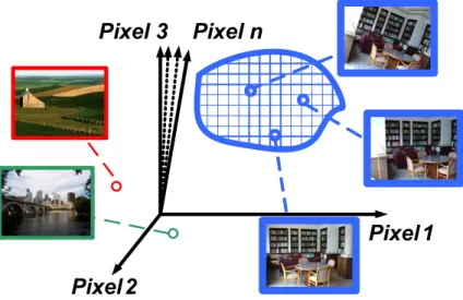
A 2D image can be considered as a point in a high dimensional appearance space (see
Chapter 3). When an object in the scene or the camera moves, the image point moves
along a certain manifold called the appearance manifold. We can see that there exists
a mapping from the pose space to the appearance manifold. Moreover, for a
non-degenerate scene, this mapping is invertible and tracking can be archived by learning
the appearance manifold. An ideal solution is to learn it globally. However, this is
usually impractical. The appearance manifold is typically highly nonlinear, and a global
learning process usually requires numerous training samples. In fact, a global learning
process is not necessary. Depending on the frame rate, the motion between two frames
is usually restricted within a certain region. Therefore a local representation of the
appearance manifold can be enough for tracking incremental motion. As discussed
earlier, an appearance manifold is defined by its underlying motion. Since motion lies in
a low dimensional space, the dimensionality of the appearance manifold is low. Therefore
it should be possible to compute a linearization of the local appearance manifold with
a small number of local image samples.
Based on the above observations, I present a framework that tracks incremental 3D
rigid motion by sampling and linearizing the local appearance manifold. Local
appear-ance samples are acquired using a camera cluster at run time. Using these samples,
a linear approximation of the local appearance manifold is computed. Motion
estima-tion is then achieved by solving a linear system. This method does not require any
prior scene model or off line training process. It does not assume any 3D or 2D
corre-spondence, thus can accommodate scenes with view-dependent appearance changes. As
far as I know, this is the first motion estimation approach that addresses challenging
scenes that exhibit complicated behaviors like semitransparancy, specularity and curved
reflections.
1.4
Thesis statement and main contributions
Thesis Statement
A 2D image can be considered as a point in a high dimensional appearance
space. When the camera or a rigid object in the scene moves, the image point moves
along a 6D appearance manifold. While globally nonlinear, the appearance manifold
can be locally linearized using a set of 7 neighboring image samples. Such a local
linearization of the appearance manifold can be used for 3D motion segmentation
and tracking.
The main contributions of this thesis work can be summarized as follows:
I A novel appearance based differential framework for tracking 3D rigid motion. The local appearance manifold is linearized using a small number of
image samples captured by a camera cluster. Tracking is effectively achieved by
solving a linear system. This approach does not require any offline scene model
or training images; nor does it assume any 3D or 2D correspondence. To my
knowledge, it is the first method that accommodates scenes with view-dependent
appearance changes. This framework can be integrated into a model-based
frame-work. When a prior graphics model is provided, the local samples can be acquired
through graphical rendering.
II A spectral analysis of the linearization of a local appearance manifold.
Any linearization of a non-linear function can only be considered valid within a
local region. To quantitatively determine the size of the local region, I formulate
the linearization as the process of sampling and reconstructing the appearance
sig-nal. The Fourier analysis shows that to avoid aliasing, the image motion between
other approaches that assume local linearization, for instance, optical flow.
III A pure appearance based approach to dense motion segmentation. This
approach is also based on a local linearization of the appearance function. The
change of the intensity of a pixel can be considered as a linear function of the
motion of the corresponding imaged surface. When a sequence of local image
samples are captured, the intensity changes of a particular pixel over the sequence
form a vector calledintensity trajectory. The intensity trajectories of pixels
corre-sponding to the same motion span a linear subspace. Thus the problem of motion
segmentation can be cast as that of clustering local subspaces.
1.5
Thesis outline
The thesis is organized as follows. A review of various approaches to motion estimation
is given in Chapter 2. Depending on their input measurements, motion estimation
methods are categorized into three classes: feature-based, flow-based and
appearance-based. Chapter 3 presents the novel framework of appearance-based differential tracking.
The algorithm of tracking by sampling and linearizing the local appearance manifold
will be introduced. Chapter 4 describes the techniques for acquiring local appearance
samples. Chapter 5 presents a spectral analysis that justifies the linearization of the local
appearance manifold from a signal process point of view. In Chapter 6, the locally linear
appearance model is applied to solve the problem of motion segmentation. Experiment
results on these new appearance-based approaches to tracking and motion segmentation
are demonstrated in Chapter 7. Finally, Chapter 8 concludes this thesis and discusses
the directions for future work.
Chapter 2
Related work
Motion estimation systems take an input image sequence and output motion parameters
of some target objects, or the camera. As described in Chapter 1, this process can be
formulated as solving a reverse mapping. An image I is a function F of the scene M
and its pose S with respect to the camera.
I =F(S, M) (2.1)
Motion can be recovered by computing one of the two reverse mappingsF−1 : from the
image I to the pose P (then subtract reference pose to current pose to get motion), or from the change of the image dI to the motion dS. 1.
S =F−1(I, M) (2.2)
dS =F−1(dI, M) (2.3)
In the above equations, I and dI are conceptually described as image and change in image. To quantitatively solve the problem, motion estimation systems extract a set
of measurements from input images and describe I and dI using these measurements.
1Note that the two functions in (2.2) and (2.3) are usually different. Here I denote both of them as
Image measurements can simply be pixel intensities or some high-level descriptors or
features computed from basic intensity values. The above equations also show that to
directly relateI toSordI todS, the sceneM needs to be decoupled. Motion estimation algorithms achieve this by acquiring some invariant representation or model of the scene.
A scene model can be an explicit one provided as a prior, or an implicit one acquired
during tracking.
This chapter will start with a brief survey of image measurements. Based on their
input image measurements, motion estimation algorithms will be categorized into three
classes: feature-based, flow-based and appearance-based. Popular methods in each of
these three classes will be reviewed. Different approaches to scene modeling will be
introduced. Finally, to conclude this chapter, a general discussion on existing motion
estimation techniques will be presented.
2.1
Image measurements
Vision-based motion estimation methods usually start by extracting measurements from
input images. Different types of image measurements have been used. Some of them
are low-level measurements that can be directly acquired from images. The most basic
image measurements are pixel intensities and intensity derivatives.
Intensity or color. The intensity or color of an image pixel is determined by the
illumination and the albedo of the corresponding surface patch. In the color
represen-tation, a variety of color spaces are used. The commonly used ones include RGB, HSV,
Luv and Lab. Among all the image measurements, intensity and color are the simplest.
However, they are sensitive to motion-dependent illumination variations hence their
us-age is usually prohibited in scenarios where the motion-dependent illumination effects
are non-neglectable.
Intensity derivative. The derivative of a pixel intensity indicates the smoothness
of the observed image at that pixel. Compared with the original intensity
measure-ments, intensity derivatives are more sensitive to imaging noise. This noise issue gets
exaggerated for high order derivatives. In practice, only the first and the second
or-der or-derivatives are used, and they are usually used as intermediate measurements for
computing some high-level measurements like textures or optical flow.
The intensity and intensity derivative measurements have the advantage that they
can be acquired with minimal computation power. However, being the simplest
mea-surements, they are in general not very descriptive to the uniqueness of the scene. To
achieve a better representation of the scene, motion estimation system usually employ
further processing of the basic image measurements to form high-level descriptors or
features. A list of commonly used high-level descriptors are presented as follows.
Intensity statistics. The probability density of the pixel intensities inside an
im-age region provides a unique description of the appearance of the object corresponding
to that region. The intensity statistics can be parametric such as a Gaussian Mixture
(RMG98), or nonparametric such as color histogram (HVM98). Like the original
inten-sity measurements, inteninten-sity statistics are usually sensitive to illumination changes.
Texture. As an image measurement, texture is usually defined as the variation
pattern of pixel intensities within a processed image window. Texture measurement
can be used to quantify the smoothness and regularity of the imaged surface. The
difference between a texture and an intensity statistic is that the latter only represents
color information while the former also records structure information. Some example
texture descriptors are wavelets (LK89) and steerable pyramids (GBG+94). Compared
with pixel intensity or color, texture measurements are usually considered less sensitive
to illumination changes.
Interest point. Interest point features are the most widely used image features
in the area of tracking. Popular point feature detecting algorithms include the Harris
detector (Low04). An overview of the state of the art in feature extractors is given by
Mikolajczyk and Schmid (MS05). In general, point features extracted by these
algo-rithms are invariant to smooth illumination changes. As a comparison, Harris features
and KLT features are invariant to translation, rotation and uniform scaling in the spatial
domain, but are not invariant to affine and projective projections. SIFT features are
more robust to different transformations, but the SIFT detector is also relatively slow
for real time tracking.
Edge. Edges correspond to discontinuities in image intensities. Possible causes of
edges include discontinuities in depth, discontinuities in surface normals, and changes
in material properties. An edge can be detected using an edge detector, which
usu-ally uses intensity derivatives. One of the most efficient and popular edge detectors is
Canny (Can86). A review of edge detecting techniques can be found in (ZT98). Edge
features are usually insensitive to illumination changes. However, edge features can
cause difficulties for tracking in an image sequence where the viewpoint changes. This
is because the occlusion relationship are view-dependent. Hence, edges caused by depth
discontinuities may change substantially when the viewpoint changes.
Optical flow. Optical flow refers to the dense 2D displacement field that indicates
the pixel motion on the image plane. For each pixel, its flow is the 2D projection of the
3D motion of its corresponding 3D scene point. The flow field is usually computed under
the brightness constancy assumption. Popular optical flow techniques include differential
methods by Lucas and Kanade (LK81) and Horn and Schunk (HS81), region-based
matching by Anandan (Ana89) and phase-based correlation by Fleet and Jepson (FJ90).
The readers are referred to the survey by Barron et al. (BFB94) for an evaluation of
optical flow methods. Optical flow is a commonly used image measurement for recovering
motion and scene geometry. However, like pixel intensities, optical flow measurements
are sensitive to illumination changes. Moreover, since optical flow is usually computed
across a local region, the flow estimates are noisy at occlusion boundaries.
So far, I have introduced a list of popular classes of image measurements. Among
them, interest point and edge features represent the 2D projections of 3D geometric
primitives. As they describe the structure and shape of the underlying 3D scene, I
cate-gorize them as geometric features. Similarly, I categorize intensity, intensity statistics
and texture as appearance measurements, since they describe the appearance of the
scene. The optical flow measurement is unique in that it directly encodes motion
in-formation. So I separate it from the other image measurements and classify it as flow
measurements.
In accordance with the three classes of input measurements, I categorize motion
estimation methods into: feature-based,flow-based andappearance-based. In the
remainder of this chapter, I will discuss each of them in details.
2.2
Feature-based motion estimation
In a feature-based framework, the scene is represented as a collection of 3D geometric
entities whose projections are observed in images as 2D features. Feature-based motion
estimation systems use the positions of these 2D features to compute the change of the
relative pose between the camera and the scene. To relate the 2D feature positions with
the 3D pose parameters, they usually assume some knowledge about the scene structure,
or more precisely, the 3D shapes and positions of the geometric entities. Such a scene
structure can be provided explicitly as a prior model or be recovered simultaneously
during tracking.
2.2.1
Model-based approaches
Most model-based approaches assume an explicit model that defines the 3D shapes and
positions of a set of geometric entities of the scene in some global coordinate system.
im-age. Motion estimation is then formulated as the single-view 3D-to-2D pose estimation
problem. The relative pose between the camera and the scene at each frame can be
estimated by computing the projective transformation that best maps the model from
its own 3D coordinate system to its current 2D image observations. Motion can then
be acquired by subtracting pose estimates.
One way of acquiring a scene model is by adding fiducials ormarkersinto the scene.
Some commonly used fiducials include color-coded rings (SHC+96; CN98) and
Light-emitting Diodes (LEDs) (WBV+01; BN95). In general, fiducials are some artificial
markers whose 3D positions in the world coordinates are precisely measured by some
offline process. These markers are designed such that they can be detected easily in
the images and their image locations can be measured to a high accuracy. Therefore,
fiducials provide easily detectable and accurate 3D-to-2D point correspondences. These
correspondences can then be used to compute poses and motions in a relatively reliable
and accurate manner. Due to such advantages, fiducial-based techniques have been
widely used in Virtual Reality and Augmented Reality.
Fiducial-based techniques require instrumenting the scene. This task can be tedious
or even impractical, especially for outdoor environments. Therefore, it is usually more
convenient to rely on natural features present in the environment. While in theory any
image feature that is detectable and measurable can be used, most practical motion
esti-mation systems employ linear primitives such as interest points (Alt92; GRS+02; VLF04)
or lines (Low87; Low92; NF93; Jur99; CMC03) or both (LHF90; HN96). There are two
major reasons for the popularity of point or edge based methods. First, methods using
simple linear primitives are computationally efficient and relatively easy to implement.
Moreover, interest point and edge features are usually insensitive to illumination
vari-ances. To establish 3D-to-2D correspondences, the 3D positions of the points and lines
need to be provided. This 3D information can be in the form of an off line CAD model
built by commercial products, or can be acquired by triangulation of several key frames
with known poses during the initialization process. The fitting of higher order
prim-itive models to their 2D projections have also been explored. For instance, quadratic
primitives have been used in (Wei93; FPF99). In comparison with linear primitives,
quadratic primitives provide more geometric constraints about the viewing parameters.
However they are usually difficult to identify and extract from images in an accurate
and reliable manner.
Fiducials and natural features can be used in a complementary way. An example was
given in an early work of Bishop (Bis84). Noticing the task of motion estimation can be
simplified by accelerating the imaging-processing-imaging circle 2, Bishop designed and
fabricated a self-tracking system using multiple out-viewing VLSI chips that performed
both imaging and processing. This integrated system used the natural features to
esti-mate incremental motion at a very high framerate. Fiducials were used to address the
drifting of the pose estimated by integrating the motion.
Estimating pose parameters
The viewing parameters can be computed from the correspondence between a set of
geometric entities with known 3D positions and their 2D projections. This so-called
3D-to-2D pose estimation problem is one of the oldest problem of computer vision. Usually
the pose parameters are estimated by maximizing an objective function that quantifies
the 3D-to-2D alignment. Due to the large number of proposed algorithms, a complete
survey of pose estimation is beyond the scope of this dissertation. Readers can refer
to (LF05) and Chapter 20 of (Se07) for detailed reviews. Here, I will briefly introduce
several of the most popular point-based approaches. The problem is formulated as:
given correspondences between a set of n 3D points Mi = [Xi Yi Zi]T and their 2D
projections mi = [xi yi]T, compute the projection matrixP that best mapsMi to mi. 2Shorter imaging time results in a higher framerate, which results in a smaller motion, which results
Direct Linear Transformation (DLT) . As shown in (2.4), each correspondence
between Mi and mi defines two equations on the elements of P. Based on this
ob-servation, DLT algorithms such as (Sut74; Gan84) solve the 11 entries of the camera
projection matrix from at least six corresponding points.
xi = (P11Xi+P12Yi+P13Zi+P14)/(P31Xi+P32Yi+P33Zi+P34)
yi = (P21Xi+P22Yi+P23Zi+P24)/(P31Xi+P32Yi+P33Zi+P34)
(2.4)
DLT is usually used as a camera calibration technique that determines both the pose
and the camera intrinsic parameters up to a scale. This over-parameterization usually
introduces instability and requires more correspondences for the purpose of pose
esti-mation. In this case, it is usually preferable to estimate the camera intrinsic parameters
separately.
Perspective-n-Point (PnP) . When camera intrinsic parameters are known, cor-respondences of 3 points can be used to estimate pose parameters with up to 4 solutions.
Additional point correspondences are required to guarantee a unique solution. (FB87)
shows that the solution is unique for 4 points on a plane or 6 points in general positions.
Depending on the number of points used, the problem is known as P3P, P4P or in the
general form PnP. Different approaches to PnP have been proposed (HLON91; QL99).
They usually employ the constraints defined by the triangle equations shown in (2.5).
d2
ij =d2i +d2j −2didjcosθij
cosθij = (mTi Qmi)/((mTi Qmi) 1
2(mT
jQmj)
1
2)
(2.5)
Here dij = kMi −Mjk, di =kMi −Ck and dj = kMj −Ck respectively represent the
distances between the reference pointsMi,Mj and the camera centerC. θij is the angle
between the viewing lines CMi and CMj. For known camera intrinsic matrix K, the
directions of CMi and CMj can be written as K−1mi and K−1mi. cosθij can the be
computed using the image projections mi,mj and matrix Q= (KKT)−1.
Gold Standard method. DLT and PnP algorithms are fast and can be solved
in closed form. However, they achieve pose estimation by minimizing algebraic error
that has no direct geometric meanings, thus are usually sensitive to measurement noise.
When the error of image measurements mi are independent and Gaussian, the optimal
pose estimate can be computed by minimizing the sum of the reprojection errors in
(2.6). This nonlinear optimization is typically solved in a iterative form. The initial
pose estimate is usually provided by one of the DLT or PnP algorithms.
[R, T] = argmin
(R,T)
X
i
kP Mi−mik2 (2.6)
2.2.2
Structure from motion approaches
So far, we have assumed that the 3D structure of the scene is provided in terms of
a prior model. For a rigid scene, its structure can also be acquired simultaneously
during tracking. This problem is referred to as SFM in computer vision. Given a set of
images of a rigid scene taken from different perspectives, SFM algorithms recover the
3D scene structure along with the camera motion across the image sequence. Depending
on the input image measurements, SFM methods can be categorized into feature-based
and flow-based. In this section, I will discuss the feature-based SFM. The flow-based
approaches will be introduced in the next section.
Feature-based SFM considers a set of 3D features undergoing rigid motion with
respect to the camera. Given the correspondences of 2D projections of the features
across multiple perspectives, SFM systems estimate the positions of the features and
the relative motion between the views, using the so-calledepipolar geometry constraint.
Commonly used features include interest points and line segments. Methods using the
two classes of features are comparable in computational complexity. The former is the
choice for most state of the art SFM systems as the real world usually consists of a
Our discussion here will focus on point-based methods. Some line-based examples can
be found in (TK95; ZF92). For a comprehensive introduction to both classes, interested
readers are referred to the multi-view geometry books by Hartley and Zisserman (HZ00)
and Faugeras and Long (FL01).
The projections of a 3D point in a rigid scene into two views are related by the
epipolar geometry constraint, which can be linearly formulated as:
m1TF m2 = 0 (2.7)
Here m1 and m2 are the image coordinates of the 2D projections of the same 3D point
M observed in two views. The 3×3 singular matrixF is called thefundamentalmatrix. Given the camera intrinsic matrixK, F can be used to compute theessential matrixE:
E =KTF K (2.8)
The estimation of the essential matrixE is the key to SFM algorithms. Once estimated,
Ecan be factorized to acquire the relative motion (the rotation and translation) between the two views. The 3D position M can then be easily acquired by triangulation. Note that the linear constraint in (2.7) is only defined up to a scale. The same scaling applies
to the recovered scene structure and the translational component of the motion.
The recovery of the essential matrix using the epipolar geometry was first proposed by
Lounget-Higgins. The so-called 8 point algorithm presented in (LH81) has the appealing
property of being linear. However, the results obtained using this approach are usually
not satisfactory in the presence of noise. From a numerical point of view, Hartley showed
that the stability of the 8 point algorithm can be improved by a simple renormalization
of the input measurements (Har97). The performance can be further improved by using
more points and adopting least square techniques, or enforcing rank (Har97) and Degrees
of Freedom (DOF) constraints (HN94; TBM94), or employing nonlinear optimization
(LF96). A review of these techniques is provided in (Zha98).
The performance of SFM can be improved by combining information from more
than two views. For instance, the feature correspondences across a triplet of images
is constrained by a trifocal tensor (SW95). When feature correspondences across a
relatively large number of views are available, the optimal structure and motion can be
estimated by solving a large nonlinear optimization problem known asbundle adjustment
(TMHF00). The objective function is the sum of square of the reprojection error of all
features from all views. Probably the most interesting technique in multi-view geometry
is the simultaneously recovery of camera intrinsic parameters along with motion and
structure, a technique called auto-calibration. Robust systems have been demonstrated
in (PKG98; Nis03). A nice introduction to these techniques, as well as a comparison
between the flow-based and the feature-based SFM approaches, can be found in (Zuc02).
2.3
Flow-based motion estimation
The termoptical flowrefers to the dense displacement field that indicates the pixel
mo-tion across frames. For each pixel, its flow is the 2D projecmo-tion of the 3D momo-tion of its
corresponding scene point. Flow-based systems thus attempt to recover the underlying
3D motion from its 2D projection. This is usually achieved simultaneously with the
recovery of the scene structure. While flow-based methods are akin to feature-based
methods in the sense that both rely on (dense or sparse) image correspondences, these
two approaches are quite different. Feature-based methods are based on epipolar
geom-etry. They can, and are better at, recovering large motions. Flow-based methods, as we
will discuss soon, use a locally linear model that is only valid for a small motion.
Under perspective projection, the flow of a pixel undergoing a small motion can be
translation and rotation of the relative motion between the scene and the camera. For
a pinhole camera model with focal length f
[u, v]T =AT /z+BR
A= ¯ ¯ ¯ ¯ ¯ ¯ ¯
−f 0 x
0 −f y
¯ ¯ ¯ ¯ ¯ ¯ ¯ B = ¯ ¯ ¯ ¯ ¯ ¯ ¯ xy
f −(f +x
2
f ) y
(f+ yf2) −xyf −x
¯ ¯ ¯ ¯ ¯ ¯ ¯ (2.9)
Equation (2.9) shows that the flow field is related to two sets of parameters: theglobal
parametersT andRthat indicate the cameramotion, and thelocal(per pixel) parameter
z that indicates the 3D structure or depth of the scene. Based on this observation, researchers have developed many optical flow based motion estimation methods. These
methods usually consist of two steps: first computing optical flow from input image
sequences, then simultaneously recovering structure and motion from flow estimate.
In the rest of this section, I will discuss the two steps accordingly, starting from flow
estimation.
2.3.1
Flow estimation
The estimation of optical flow is based on the brightness constancy assumption (HS81).
The brightness constancy assumption states that the brightness of a moving object
re-mains constant and the change of the image intensityI(x, y, t) is a result of a translation in the image plane.
I(x+u, y+v, t+4t) =I(x, y, t) (2.10) where (x, y) are the coordinates of image pixel, (u, v) are the image displacement or flow of pixel (x, y) between the two images taken at time t and t+4t respectively. From the first order Taylor’s expansion of (2.10), the well-known gradient constraint equation
can be written as
Ixu+Iyv+It= 0 (2.11)
where (Ix, Iy) are the spatial derivatives and It is the change of pixel intensity at (x, y).
Different techniques have been developed to estimate flow field (u, v). Based on the types of extracted image measurements, optical flow algorithms can be categorized
into four classes: differential-based, energy-based, phase-based and correlation-based
(BFB94). Here I will briefly introduce the more commonly used differential and
correla-tion methods. Interested readers can refer to (BFB94) for a detailed review. Evaluacorrela-tions
of optical flow methods can be found in (LHH+98; BRS+07).
Differential-based methods
Differential-based methods compute the flow field using (2.11). Since (2.11) only
pro-vides one constraint to two unknowns, we need to introduce other constraints to compute
(u, v). Horn and Schunk (HS81) combined a global smoothness term with the gradient constraint equation to form an objective function for flow estimation.
X
D
(Ixu+Iyv+It)2+λ(u2x+u2y+vx2+vy2) (2.12)
The flow field can then be solved iteratively by minimizing the objective function. In
(2.12), D represents a local region, and (ux, uy, vx, vy) are the flow derivatives that
indicate the smoothness of the flow field inside D. Thus the second regulation terms can be expressed as the flow field is smooth within the local region.
Similarly, Lucas and Kanade (LK81; Luc84) added a global smoothness constraint
by assuming constant flow within a local region. The objective function becomes
X
(x,y)∈D
W2(x, y)[Ix(x, y)u+Iy(x, y)v+It(x, y)]2 (2.13)
whereW(x, y) represents a window function that gives more weight to center pixels than the periphery ones. The flow field is then solved linearly in the least-square form.
lo-cal region. The underlying assumption is that neighboring pixels are likely to correspond
to the same surface. When the surface is smooth the flow field should change smoothly.
Most differential-based methods employ this assumption. Clearly, this smoothness
con-straint is likely to be violated when the examined local region crosses surface boundaries.
Correlation-based methods
The most direct way to compute flow field is to match regions from the previous image
to the current image. In this type of methods, the flow field is assumed to be constant
within a local neighborhood. This formulation is similar to area based stereo
correla-tion. The flow estimate can be computed by finding the best match that minimizes a
distance function. For example, Anandan (Ana89) and Singh (Sin92) use Sum-of-square
Difference (SSD) as the distance function shown in (2.14).
X
(x,y)∈D
[I(x+u, y+v, t+4t)−I(x, y, t)]2 (2.14)
The correlation-based methods again assume constant local flow field. The underlying
assumption is that the intensity pattern of a small region is likely to remain constant
over time, even when its position changes. This assumption can be violated, for instance,
when the local region contains motion boundaries or when the change of illumination
occurs.
2.3.2
Motion estimation
Equation (2.9) shows that the flow field provides constraints to two sets of parameters:
the global parameters that indicate the camera motion and the local (per pixel)
param-eters that indicate the 3D structure of the scene. It follows that both the structure
and the motion can be recovered from the estimated flow field in an iterative form. In
the absence of noise, the motion parameters can be recovered using the flow and depth
measurements at five or more pixels (Hor87). In practice, as the per-pixel flow estimate
is usually noisy, more points are needed. Thus the structure from motion problem is
usually solved using a least-square optimization scheme (ZT99; BH83; HJ92).
Bruss and Horn (BH83) proposed a method to estimate ego-motion by minimizing
the sum-of-square of the optical flow residual r = [u∗, v∗]T − [u(T,Ω, z), v(T,Ω, z)].
The least-square estimate of the depthz and the rotation Ω are computed as a function of translation T. These estimates are then substitute back to the residuals to form a function of the translation alone. A nonlinear solver is then applied to estimate T, z
and R are then computed.
Heeger and Jepson (HJ92) proposed to estimate egomotion using subspace
meth-ods. Similar to (BH83), they used algebraic manipulation to separate the
computa-tion of translacomputa-tion from those of the depth and the rotacomputa-tion. However, they avoided
the nonlinear optimization process required for computing the translation. Under the
instantaneous-time assumption, for a given set of optical flow at n pixels they con-structed m−6 constraint vectors that are orthogonal to the camera translation. Thus the translation can be computed in a linear form.
2.3.3
Direct methods
The above methods recover structure and motion parameters using (2.9). The
esti-mation accuracy depends on the quality of the input flow field. Unfortunately, as
we have discussed, the computation of the optical flow is usually error prone. To
address this issue, researchers have developed methods that bypass flow estimation
(IA99; Ira02; Han91; HO93). The so-called direct methods solve two problems
simul-taneously: the estimation of structure and motion, and the estimation of optical flow
(pixel correspondence).
Direct methods use the gradient constraint provided in (2.11). Using some
motion parameters and the local shape parameter. A set of n pixels provide n gradient constraints ton+5 unknowns: nlocal shape parameters plus 6 DOF rotation and trans-lation minus 1 DOF scaling factor. To solve this ill-posed problem, more constraints
need to be added. There are two general approaches to additional constraints: assuming
smoothness of scene depth (Han91), or using multiple frames (IAC02). For instance,
3 frames (two motions) of n pixels provide 2n constraints for the n + 11 unknowns. Note that the latter approach also assumes local smoothness. This is determined by the
use of (2.11), which is only applicable to small (sub-pixel) motion. To accommodate
practical image motion that is almost always larger than a pixel, direct methods smooth
the original image to acquire a filtered image with enlarged pixel size. The underlying
assumption is that the 3D scene patch corresponding to an enlarged pixel is of constant
depth and therefore uniform flow velocity. As we have discussed, the local smoothness
assumption can be violated at occlusion boundaries. Therefore, the application of
di-rect methods is usually constrained to close-to-planar scenes, where the motion can be
described using simple parametric form such as affine or quadratic (TZ99).
2.4
Appearance-based motion estimation
The scene appearance in the 2D camera images changes with respect to the motion
be-tween the scene and the camera. The key to 3D appearance-based tracking is to acquire
some appearance model that can parameterize this relationship. There are two general
approaches to 3D appearance-based tracking. One approach utilizes a 3D renderable
model that can be used to predict the scene appearance from different hypothesized
views. Motion estimation is achieved by matching the real image appearance with the
predicted ones. The other approach learns a parametric representation of the scene
ap-pearance using a set of training images. The motion estimate is computed by projecting
current appearance observation into that parametric space.
Many appearance-based motion estimation algorithms aims at solving the problem
of visual tracking in a 2D scenario. The goal is to consistently locate the image region
occupied by a specific target in each frame of the input image sequence. Typically, the
target object is represented using an appearance model that describes some invariant
image property. Popular appearance models include global statistics such as mixture
model (Fre00) or color histogram (CRM00), and texture such as wavelets (JFEM03).
A major advantage of these models is that they can be acquired on line with minimum
effort. The models are usually initialized using a small number of (usually one) frames
and can often be refined during tracking. However, these appearance models are
inher-ently 2D, and only encode information on object appearance changes with respect to an
image or an affine motion.
2.4.1
Model-based approaches
For 3D tracking, some kind of 3D appearance representation is required to predict
the appearances of the scene from different views. A popular class of approaches to
tracking objects under changing views employs textured 3D graphical models of target
objects. The appearance of the object at some predicted pose is generated through
graphics rendering. Dellaertet al. (DTT98) proposed a Kalman filter based system that
simultaneously estimates the pose and refines the texture of a planner patch. Cascia
et al. (CSA00) used a textured cylindrical model for head pose estimation. Schodl
(SHE98) and Chang (CC01) used a textured polygonal model for more accurate head
pose estimation. An appealing property of a textured 3D model is that it can be rendered
efficiently using graphics hardware. This advantage has made it the choice of most
existing model-based methods. In theory, any model that can be used to synthesize
appearance samples from different views can be used. For instance, a pre-acquired
lightfield model is used in (ZFS02).
usu-ally different from the on line condition. Since the appearance of an object changes
with respect to the illumination, model-based methods are prone to the illumination
in-consistencies between the modeled and the real spaces. Different techniques have been
developed to address the illumination issue. In (CC01), the change of illumination is
addressed by using local correlation coefficients as the similarity measurements. Hager
et al. (HB98) and Cascia et al. (CSA00) used a linear subspace to model the change
of appearance under varying lighting conditions. Zhang et al. (ZMY06) proposed the
use of belief propagation to estimate the intensity ratio between corresponding pixels
of an image pair. They applied this illumination insensitive method to visual
track-ing. In (YWP06), we addressed model-based 3D tracking of Lambertian objects under
directional light sources. A Kalman filter framework is applied to estimate the object
motion, the illumination and refine the texture model simultaneously. This illumination
insensitive model-based method is described in Section 4.2.
Acquiring an off line model can be tedious and sometimes impractical, for instance,
consider camera tracking in an outdoor environment. Researchers thus have worked
on developing methods that can recover the 3D shape (ZSM06) and appearance model
(ZH01) from image data during tracking. While on line modeling is appealing, and can
greatly boost the applicability of model-based approaches, the state of the art algorithms
are still not robust enough in general . Tracking error usually causes the mapping of
background data into the model, which in turn results in larger tracking error. The
system therefore becomes unstable quickly. Practical model-based methods thus still
rely on an off line modeling process to provide the full 3D model of the target object or
at least an initial one to start with.
2.4.2
Image-based approaches
A parametric representation of the scene appearance can be acquired using training
image samples taken from different known perspectives. The idea is that the set of
all possible images of the target object lie on a low-dimensional manifold that can be
parameterized by the varying pose and illumination parameters.
Pioneered by the work of Murase and Nayar (MN95), a popular class of algorithms
models scene appearance using linear subspaces. Usually, the appearance subspaces
are computed by applying Principal Component Analysis (PCA) to a set of collected
training images with known pose and illumination parameters.
Consider an n-pixel image I, which can be considered as a vector point in the high dimensional space Rn. At the training stage, a set of m images Ψ = [I
1, I2, ..., Im] are
taken from different poses Θ = [θ1, θ2, ..., θm] under different illumination conditions
Ω = [ω1, ω2, ..., ωm]. We can compute the eigenvalues λi and eigenvectors Vi by
apply-ing eigen-decomposition of the n×n covariance matrix Q = ΨΨT. The eigenanalysis
provides an efficient way of dimension reduction. As the image is a function of the
pose and illumination parameters, the appearance manifold is low-dimensional. We can
approximate the nonlinear appearance manifold using the linear subspace spanned by
the firstk eigenvectors3. More specifically, the least square approximation ˜I of the real
image I can be computed as
˜
I =
k X
i=1
ciVi (2.15)
where ci =I·Vi represents the coordinate (projection) of the image in the appearance
subspace spanned by the eigenvectors Vi. We can project all training images into the
appearance subspace and acquiremdiscrete samples with known poseθand illumination
ω parameters. A parameterization of the appearance subspace (θ, ω) = Φ(c1, c2, ..., ck)
can then be computed from the discrete samples through, for instance, interpolation.
During tracking, the input image is again projected into the appearance subspace. The
pose and illumination parameters can be recovered using Φ.
The linear subspace model is first applied to object recognition by Murase and
Na-3Due to the highly nonlinear nature of the appearance manifold, k is usually chosen to be larger
yar (MN95). They also demonstrated tracking 1D rotation of a rigid object. Later,
Hager and Belhumeur (HB98), and Black and Jepson (BJ98) applied the appearance
subspace model to visual tracking of rigid and articulated object respectively. The linear
appearance model is simple and computationally efficient. However, globally
approxi-mating a nonlinear function using linear representation is fundamentally problematic.
Systems adopting this linear model require higher dimensional parameters to model the
underlying low dimensional nonlinear manifold. While projecting the problem to higher
dimensions can reduce approximation errors, it also enlarges the search space and causes
the optimization to be less stable. Moreover, as the dimensionality increases, the number
of training images usually increases dramatically. The training process then becomes
extremely tedious. For building a model for one specific target, it already involves tens
if not hundreds of tuning and recording of the pose and illumination parameters.
To address the nonlinearity of the appearance manifold, a number of researchers
have proposed to learn a nonlinear mapping between the image appearance and the
pose parameters. For instance, Rahimi et al. (RRD05; RRD07) and Elgammal (Elg05)
proposed to approximate the appearance function using a series of Radial Basis
Func-tions (RBF). In theory, given enough input-output examples, any smooth nonlinear
function can be learned using a family of functions such as RBF. However, that number
ofenough examples is usually high for a close approximation. For instance, 125 training
images are used in (Elg05) to track an rigid object undergoing affine motion. To reduce
the number of examples, a semi-supervised learning process that leverages the temporal
coherence of video sequence is proposed in (RRD05). The authors reported tracking of
a synthetic cube undergoing 3D rotation under a constant illumination. The training
dataset includes 6 manually selected supervised images plus 1496 unsupervised images.
Tested using the same training data, a mean estimation error of 4 degrees is reported.
In a closely related area, the problem of manifold learning has been actively studied
recently. Manifold learning techniques recover the low-dimensional structure embedded
in the high-dimensional data. Usually, this is achieved by mapping the high-dimensional
input data to low-dimensional global output coordinates, while preserving the local
re-lationship between data points. For instance, Isomap (TdSL00) preserves the
geodes-tic distances between local points, and LLE (RS00) preserves the linear interpolation
weights between local points. The local neighborhood is defined by thresholding the
pairwise distances between data samples. Clearly, the manifold needs to be densely
sampled. Otherwise, neighboring points along the manifold are difficult to identify, the
algorithms will then fail to recover the underlying structure. Experiment results show
that, given enough training samples, these algorithms can almost always learn an
accu-rate mapping from the high-dimensional data space to the low-dimensional parameter
space. However, due to the requirement of dense sampling, it is impractical to apply
learning methods to appearance-based 3D tracking. The study of manifold learning
techniques, especially LLE, justify and emphasize that an age-old strategy also applies
to appearance manifold: approximating a globally nonlinear function can be
done with a piecewise locally linear representation .
2.5
Discussion
Feature-based approaches describe the scene as a collection of 3D geometric primitives
such as points or lines. For model-based approaches, the 3D positions of these primitives
in some global coordinate are given as priors. Motion is recovered by solving a
3D-to-2D pose estimation. By estimating the pose rather than the motion, model-based
methods efficiently eliminate error accumulation. However, acquiring offline models can
be tedious and sometimes infeasible, for instance, outdoor camera tracking.
In a different approach, feature-based SFM methods apply the epipolar constraint to
corresponding features across multiple frames. The scene structure is recovered during
feature-based SFM methods are prone to drifting. This issue, however, is well-balanced
by the convenience of online modeling. Besides, with the development of multi-view
techniques such as bundle adjustment, modern SFM systems have been able to track
over a long period of time with little drift. The real challenge to feature-based SFM
techniques comes from the task of corresponding features. Identifying and matching
features in different views are hard in general, and can become really difficult in scenes
presenting view-dependent appearance. For instance, scenes with occlusion boundaries,
curved reflective surface, semitransparent surfaces, and specular reflections all change
appearance dramatically as the viewpoint changes. Moreover, algorithms adopting the
epipolar constraint are numerically unstable for small feature displacements. Therefore
feature-based SFM methods usually generate less accurate results when estimating small
scale motions.
Based on a local linear model, flow-based SFM systems handle small motions. Like
feature-based approaches, they do not require a prior model of the scene. Motion and
scene structure are both recovered using dense optical flow field. The performance of
flow-based methods is usually restricted by the noisy input flow field. To compute flow
estimates, flow-based methods usually make two assumptions: constant intensity and
locally smooth depth. For simple scenes, 4 the constant intensity assumption can be
considered valid under small motion. The assumption about local depth smoothness is
usually violated at occlusion boundaries. Therefore, the application of flow-based SFM
methods is usually restricted to scenes with smooth surfaces, or distant and
close-to-planar scenes where an affine projection model can be used.
Appearance-based methods utilize the entire appearance observation. Compared
with feature or flow measurements, appearance (intensity) measurements are easier to
acquire. The computation time for feature extraction is eliminated, and the difficult
4Here normal indicate that the scene surface does not present complicated photometric properties,
such as specularity or semi-transparency.
correspondence problem is avoided. Despite all of these advantages, appearance-based
methods still receive less publicity among vision community. I believe this unpopu-larity is, to a large extent, due to the difficulty of globally modeling scene
appearance. Existing 3D appearance-based methods assume an offline global
appear-ance model of the scene. Such a global model is hard to acquire. Hundreds of training
images need to be captured, all at known poses. Moreover, aside from poses, the scene
appearance is also largely determined by illumination. Since illumination changes
be-tween the offline modeling stage and online tracking stage are usually inevitable, more
training images need to be captured to accommodate this variation. Besides, adding
il-lumination parameters projects the problem into a higher dimension. Estimation in this
enlarged searching space becomes less stable. One day, these difficulties of global
ap-pearance modeling may eventually be solved, probably with a new generation of imaging