FUNDAMENTAL PROPERTIES OF WHITE DWARFS ALONE AND IN BINARIES
Joshua Thomas Fuchs
A dissertation submitted to the faculty at the University of North Carolina at Chapel Hill in partial fulfillment of the requirements for the degree of Doctor of Philosophy in the
Department of Physics and Astronomy.
Chapel Hill 2017
Approved by:
c ○2017
ABSTRACT
Joshua Thomas Fuchs: FUNDAMENTAL PROPERTIES OF WHITE DWARFS ALONE AND IN BINARIES.
(Under the direction of J. Christopher Clemens.)
White dwarfs are physically simple and numerous. Their properties provide insight into stellar evolution and have applications to many astrophysical questions. In this dissertation, we present new measurements of white dwarf properties in two environments that help further our knowledge of the structure and evolution of white dwarfs.
We have undertaken a series of observations that enable the measurement of fundamental parameters of the white dwarf in two magnetic cataclysmic variables. We have chosen these particular systems because the lack of accretion disk and fortunate geometry leading to eclipses makes it possible to observe and characterize the white dwarf.
We have also completed a spectroscopic survey of pulsating, hydrogen-dominated atmo-sphere white dwarfs. These pulsations have long offered the promise to conduct seismology of white dwarfs to understand their internal structure and composition.
We have spectroscopically observed 122 DA white dwarfs that are either pulsating or close to the DA instability strip. We estimate Teff and logg for each white dwarf from the
shape of the Balmer line profiles. These parameters provide important initial constraints for both absolute and relative seismology. We have completed a careful study of ten systematics involved in the determination ofTeff and logg. Understanding and limiting these systematics
ACKNOWLEDGMENTS
The past six years have been a journey. Like any journey, there have been moments of triumph and joy, as well as moments of discouragement and uncertainty. Perseverance has been required, and there have been numerous people and groups that have supported and encouraged me along the way. They have helped celebrate the triumphs and provided encouragement through the moments of uncertainty.
I am thankful for the guidance and support of my advisor, Chris Clemens. In addition to the technical aspects I have learned from him, he has modeled a wonderful approach to being a scientist. His persistence in avoiding dogmatic views and his quest for deeper understanding are two of the qualities I most admire, and I hope I have acquired.
Darragh O’Donoghue is responsible for originally piquing my interest in magnetic cata-clysmic variables. I am grateful for his introduction to the field and his thoughts and advice as we sought to understand LSQ 1725-64. Most of all, I am grateful to have learned from his philosophy and approach to science and life. His sudden passing in the course of this work was tragic, and his guidance and presence have been missed.
I am also thankful for the work and assistance of my colleagues in the Clemens group at UNC: Bart Dunlap, Erik Dennihy, JJ Hermes, Jesus Meza, and Patrick O’Brien. They have provided support, feedback, and assistance for the work described here. They have also been excellent company on many observing nights and coffee trips.
I am thankful to my committee of Chris, Dan Reichart, Dean Townsley, Nick Law, and Art Champagne for their advice, willingness to serve, and having at least read this far.
Davis played formative roles in my physics education at Rhodes College. They generated in me an interest and curiosity of physics, and encouraged me to continue my studies.
All of the data presented in this dissertation comes from the SOAR Telescope, the Southern African Large Telescope, and PROMPT. I am particularly thankful to the telescope operators, day crew, and staff at SOAR for their work and assistance through many nights of observing. The Goodman Spectrograph has been the ideal instrument for this work. SALTICAM and PROMPT have enabled discoveries that would not have otherwise been possible.
Financial support has been provided by two main sources. The National Science Foun-dation, through grant AST-1413001, has allowed me to focus on research the past three years. My first three years I was supported as a Teaching Assistant. I am thankful to the taxpayers of the state of North Carolina for their support in that work. Along that line, I am also thankful to Jennifer Weinberg-Wolf, Alice Churukian, and Duane Deardorff for teaching me how to teach effectively.
Computational support has been provided by the Renaissance Computing Institute and Steve Cox. I am thankful to them for helping to significantly speed up the white dwarf fitting discussed in chapter 4. The white dwarf models were provided by Detlev Koester. I am thankful to him for his many years of work on the models and making it possible for us to undertake this project.
This work was mostly completed in Phillips Hall and Chapman Hall on the UNC cam-pus. But a number of other locations have also provided a place to sit, think, converse, program, write, and drink caffeine. These include Johnny’s Gone Fishing, View/360, the North Carolina Study Center, my car on the drive back from the 19thEuropean White Dwarf Workshop in Montreal, and Chris’ cabin in the Uwharrie Mountains.
also thankful to Fred and Nancy Brooks for their hospitality and involvement with Focus over many years. Many Focus events and trips have provided necessary breaks from work.
Grace Community Church has been a wonderful church home the past six years. I am grateful to the many people who have been involved in making it a nurturing community. I appreciate the value placed on deep thinking, serious conversations, hospitality, and good food.
Friends near and far have also been a source of assistance and encouragement. I appre-ciate the meals, coffee, games, movies, trips, adventures, and conversations they have been a part of. Tyler Farnsworth, Josh Welch, Alan Tubbs, Andy Garrison, and Alan Moon, in particular, have provided distractions when I needed them and focus when I needed that.
My family has been very supportive on this journey. I appreciate their willingness to learn what I do, come visit North Carolina, and support me from afar. I am thankful to my parents for raising me to be curious and encouraging me to follow my passion. I am thankful to my brothers for their support on many of my journeys. I am grateful for the sisters-in-law, brothers-in-law, nieces, nephews, and parents-in-law who have become part of the family and have greatly enriched family gatherings and provided additional sources of support.
To my dear wife Rachael, I am grateful that our journey together has been a part of this journey. You have provided words, encouragement, and support that have helped me to continue and persevere. You have expanded my comfort zone and given me room to grow. Your love has helped this work come to fruition.
TABLE OF CONTENTS
LIST OF FIGURES . . . xiv
LIST OF TABLES . . . xv
LIST OF ABBREVIATIONS AND SYMBOLS . . . xvi
1 INTRODUCTION . . . 1
1.1 Single Star Evolution . . . 2
1.1.1 Pulsating White Dwarfs . . . 4
1.2 Problems in the Measurement of Fundamental Properties of Single White Dwarfs . . . 5
1.2.1 Asteroseismology . . . 5
1.2.2 Effective Temperatures . . . 6
1.2.3 Masses . . . 7
1.3 The Physics of the Spectroscopic Determination of Teff and logg . . . 12
1.4 Plan for Measuring Properties of Single White Dwarfs . . . 15
1.5 Binary Star Evolution . . . 15
1.5.1 Magnetic Cataclysmic Variables . . . 16
1.6 Problems in the Measurement of Fundamental Properties of White Dwarfs in Binaries . . . 19
1.6.1 Masses . . . 19
1.6.2 Effective Temperatures . . . 20
1.6.3 Magnetic Field Strengths . . . 21
1.7 Plan for Measuring Properties of White Dwarfs in Binaries . . . 23
2 THE MAGNETIC CATACLYSMIC VARIABLE LSQ1725-64 . . . 26
2.1 The Interesting Properties of Polar Candidate LSQ1725-64 . . . 26
2.2 Observations . . . 30
2.3 The Magnetic Field of the White Dwarf . . . 33
2.4 Photometric Properties of LSQ1725-64 . . . 35
2.4.1 Orbital Ephemeris . . . 35
2.4.2 Photometric Variations at the Orbital Period . . . 37
2.4.3 Longterm Monitoring of Photometric States . . . 44
2.5 Spectroscopic Properties of LSQ1725-64 . . . 47
2.5.1 Continuum Measurements . . . 48
2.5.2 Emission Line Measurements . . . 54
2.6 Discussion . . . 60
2.6.1 Is LSQ1725-64 a post-bounce system? . . . 62
2.6.2 Binary Parameters . . . 65
2.6.3 Mass Transfer Rate . . . 68
2.7 Conclusions . . . 71
3 THE MAGNETIC CATACLYSMIC VARIABLE CTCV1928-50 . . . 73
3.1 The Interesting Properties of Polar CTCV1928-50 . . . 73
3.2 Observations . . . 75
3.3 Longterm Behavior . . . 76
3.4 Emission Line Profiles . . . 77
3.4.1 Radial Velocities . . . 78
3.5 Binary Parameters . . . 81
3.6 Halo Zeeman Absorption . . . 84
3.6.2 Option 2: Free-fall Velocity Near the White Dwarf . . . 87
3.7 Conclusions . . . 89
4 A SPECTROSCOPIC SURVEY OF DAVs . . . 91
4.1 Survey Design and Target List . . . 93
4.2 Observations . . . 94
4.3 Data Reduction . . . 95
4.4 Fitting Procedure . . . 100
4.5 Exploration of Systematics in the Data Reduction and Fitting Procedure . . 102
4.5.1 Flat Fielding . . . 102
4.5.2 Extinction . . . 105
4.5.3 Flux Calibration . . . 105
4.5.4 White Dwarf Model for Relative Flux Calibration . . . 106
4.5.5 Pseudogaussian Fitting . . . 107
4.5.6 Continuum Normalization Wavelengths . . . 108
4.5.7 Model Resolution . . . 109
4.5.8 Night-to-night Variations . . . 110
4.5.9 Variation with Choice of Spectral Line . . . 112
4.5.10 Variation with Choice of Line Combinations . . . 115
4.5.11 Error Budget . . . 117
4.6 Hot and Cold Solutions . . . 119
4.7 Establishing a Uniform Scale . . . 121
4.8 Results . . . 121
4.8.1 DA Instability Strip . . . 122
4.8.2 Weighted Mean Period vs. Teff . . . 124
4.9 Conclusions . . . 127
5 CONCLUSIONS & OUTLOOK . . . 128
5.1 New Characterization of Two Magnetic Cataclysmic Variable . . . 128
5.2 Careful Atmospheric Parameters of Pulsating White Dwarfs . . . 129
5.3 Future Outlook . . . 130
Appendix A ECLIPSE TIMINGS OF LSQ1725-64 . . . 132
Appendix B Teff and logg VALUES OF DAVs . . . 134
LIST OF FIGURES
1.1 Sensitivity of Line Profiles to Teff and logg . . . 10
1.2 The Solution to the High-logg Problem . . . 12
1.3 Theoretical Prediction of Zeeman Splitting of the Hydrogen Atom . . . 22
2.1 Observed Zeeman Splitting of H β in LSQ1725-64 . . . 34
2.2 SALT Lightcurve of LSQ1725-64 . . . 36
2.3 O-C Diagram of LSQ1725-64 . . . 38
2.4 Two States of Mass Transfer in LSQ1725-64 . . . 39
2.5 Low State Lightcurve of LSQ1725-64 . . . 42
2.6 Theoretical Expectation for Ellipsoidal Variation Amplitudes . . . 44
2.7 PROMPT Lightcurve of LSQ1725-64 . . . 46
2.8 PROMPT Monitoring of LSQ1725-64 . . . 47
2.9 Time-averaged Region 3 Flux in LSQ1725-64 . . . 48
2.10 Observation of the Accretion State Transition . . . 49
2.11 Spectra by Region of LSQ1725-64 . . . 50
2.12 Time-series Spectroscopy of LSQ1725-64 . . . 52
2.13 Spectral Components of LSQ1725-64 . . . 53
2.14 Trailed Spectra of LSQ1725-64 . . . 56
2.15 Hα Emission in Different Accretion States . . . 57
2.16 High State Radial Velocity Measurements . . . 59
2.17 Low State Radial Velocity Measurements . . . 61
2.18 Constraints on the Spectral Type of the Secondary Star . . . 65
3.1 PROMPT Lightcurve of CTCV1928-50 . . . 77
3.2 Longterm Monitoring of CTCV1928-50 . . . 78
3.4 Radial Velocity Measurements of the Narrow Emission-line Component
in CTCV1928-50 . . . 80
3.5 Radial Velocity Measurements of the Broad Emission-line Component in CTCV1928-50 . . . 81
3.6 Halo Zeeman Absorption in CTCV1928-50 . . . 85
3.7 Wavelength Variation of the Halo Zeeman Absorption . . . 86
3.8 Measuring the Free-fall Velocity Near the White Dwarf in CTCV1928-50 . . . . 88
4.1 g-magnitude Distribution of Observed White Dwarfs . . . 94
4.2 Flux Calibrated Spectrum of L 19-2 . . . 99
4.3 Best-fitting Normalized Models Over-plotted on Normalized Spectra . . . 100
4.4 Flat Field Options . . . 104
4.5 Changes in Atmospheric Parameters from Using Different Models for Relative Flux Calibration . . . 107
4.6 Changes in Atmospheric Parameters from Re-normalizing after Pseudo-gaussian Fitting . . . 108
4.7 Variation of Atmospheric Parameters with Different Normalization Wavelengths 109 4.8 Variation of Atmospheric Parameters with Different Resolution Models . . . 112
4.9 Line-by-line Atmospheric Parameter Results for L 19-2 . . . 113
4.10 Line-by-line Atmospheric Parameters Results for All Observed White Dwarfs . . 114
4.11 Comparing Atmospheric Parameter Results with Hα through H 10 and H β through H 10 . . . 116
4.12 Comparing Atmospheric Parameter Results with Hβ through H 10 and H γ through H 10 . . . 117
4.13 Comparing Atmospheric Parameter Results with Hβ through H 10 and H β through H 9 . . . 118
4.14 Comparing Atmospheric Parameter Results with Hβ through H 10 and H β through H 8 . . . 119
4.15 Hot and Cold Solutions from Spectral Fitting . . . 120
4.16 DAV Instability Strip . . . 122
4.18 Weighted Mean Period vs. Teff . . . 125
LIST OF TABLES
2.1 Photometric Observations of LSQ1725-64 . . . 31
2.2 Spectroscopic Observations of LSQ1725-64 . . . 32
2.3 Binary Parameters of LSQ1725-64 . . . 67
3.1 Spectroscopic Observations of CTCV1928-50 . . . 75
3.2 Binary Parameters of CTCV1928-50 . . . 83
4.1 Summary of Explored Systematics in the Data Reduction and Fitting Procedure 103 4.2 Night-to-night Variations in Atmospheric Parameters . . . 111
A.1 Eclipse Timings Used to Update the Ephemeris of LSQ1725-64 . . . 133
LIST OF ABBREVIATIONS AND SYMBOLS
AGB Asymptotic Giant Branch
DA White Dwarf with observed hydrogen lines DAV Photometrically variable DA
hDAV Hot DAV
cDAV Cool DAV
DB White Dwarf with observed helium lines DBV Photometrically variable DB
logg log of the surface gravity (cm s−2)
NOV White Dwarf Not Observed to Vary
M Solar mass
R Solar radius
SDSS Sloan Digital Sky Survey
Teff Effective Temperature
CHAPTER 1: INTRODUCTION
His imagination was full of all that he read in his books, to wit,
enchantments, battles, single combats, challenges, wounds,
courtships, amours, tempests, and impossible absurdities. And so
firmly was he persuaded that the whole system of chimeras he read
of was true, that he thought no history in the world was more to be
depended upon.
— Don Quixote
Big questions can sometimes be answered simply. White dwarfs are in many ways the simplest stars - the majority of them are composed of just four elements. These degenerate stars are the end fate of stars less than 8-10 M (Doherty et al. 2015 and Williams et al. 2009). As the most common stellar endpoint, knowing properties of white dwarfs has far ranging astrophysical applications. Measuring the structure and composition of white dwarfs provides insight into stellar evolution and nuclear physics. The luminosity function of white dwarfs provides a method to estimate the age of the galaxy (Winget et al., 1987). Initial mass - final mass relations quantify mass loss throughout stellar evolution and relate to chemical enrichment of subsequent stellar generations (Ferrario et al., 2005). In order to probe these astrophysical questions we must first understand the basic properties of white dwarfs in multiple environments.
our knowledge of hydrogen-dominated atmosphere pulsating white dwarfs by providing a consistent set of these fundamental parameters. This set of parameters will lead to better seismology of white dwarfs by constraining the two most important parameters that can be determined from spectroscopy.
Then, we will discuss the evolution of binary star systems, particularly systems that evolve into attached magnetic white dwarf - M dwarf systems called magnetic cataclysmic variables. The complexity of these systems makes it difficult to measure fundamental pa-rameters of the white dwarf, but eclipses or lower states of accretion make this possible. Our work on two such systems, presented in chapter 2 and chapter 3, provides measurements of parameters including white dwarf mass and radius as well as insight into the evolutionary history of these systems. This work is leading to a better understanding of the distribution of the types of magnetic cataclysmic variables found in nature.
1.1 Single Star Evolution
The theoretical understanding of single star evolution is as follows. After main sequence stars exhaust the majority of the hydrogen they are able to burn, they expand, become red giants, and begin burning helium. After the completion of helium burning, stars move onto the Asymptotic Giant Branch (AGB), where they become both cooler (due to increasing radii) and more luminous (due to now fusing both helium and hydrogen in different shells). On the AGB, the carbon and oxygen core that will become the future white dwarf core has already formed. It is surrounded by a thin shell of burning helium, a larger shell of non-burning helium, a thin shell of burning hydrogen, and finally the outermost envelope containing non-burning hydrogen and heavier elements.
Thermal pulses during the AGB stage determine the final structure and composition of the soon-to-be white dwarf. The hydrogen and helium shells undergo burning alternately. Every ∼ 104 years, the helium burning shell becomes unstable, which causes convection in
These thermal pulses can change both the structure of the degenerate core and the relative amounts of hydrogen and helium that will be left after the envelope is shed. The-oretically, the last shell burning before the star leaves the AGB will determine the primary atmospheric constituent (Iben, 1984). If the star leaves during hydrogen burning, it will have a primarily hydrogen atmosphere. If it leaves during helium burning, it can lose all of its helium and be left with a helium-dominated atmosphere. Iben (1984) was the first to show that AGB stars burn hydrogen roughly 80 percent of the time and helium 20 percent of the time, aligning the theory with observations of white dwarf atmospheres.
AGB stars will lose mass through stellar winds and pulsations, at a rate that can ap-proach 104 M
yr−1. As the star continues to lose mass, it enters the planetary nebula phase, where, since the hot core is continually becoming more visible, the effective temper-ature increases dramatically. This is the phase in which the star crosses the H-R diagram at a near constant luminosity to a hotter effective temperature and becomes a single white dwarf.
The small size (∼0.01 R) and relatively large mass (∼0.6 M) of white dwarfs means they have large surface gravities, typically around logg of 8.1 This causes the atmosphere to be radially stratified by element. White dwarfs are further classified by the primary observed atmospheric constituent, following the system described by Sion et al. (1983). Those with hydrogen-dominated atmospheres are classified as DA white dwarfs. Those with helium-dominated atmospheres are DB white dwarfs, or DO white dwarfs in the case of ionized helium. White dwarfs with carbon-dominated atmospheres are called DQs. White dwarfs with no obvious spectral features are called DC white dwarfs. Furthermore, white dwarfs with detected metals in their atmosphere are called DZ white dwarfs. Given the large surface gravities, the presence of DBs suggests that those stars have very little hydrogen at all. Likewise, DZs must be either polluted by an external source, commonly believed to be the remnants of extra-solar planetary systems (see the recent review by Farihi 2016), or in
the case of hotter white dwarfs, radiative levitation can keep some heavy elements close to the photosphere. Roughly 83 percent of white dwarfs are DAs, 15 percent DBs and DOs, with DCs, DQs, and DZs providing the remainder (Eisenstein et al., 2006).
1.1.1 Pulsating White Dwarfs
Photometrically variable white dwarfs were first discovered by Landolt (1968), who found HL Tau 76 to be variable in his search for good non-variable standard stars. It took a few more discoveries of variable white dwarfs (see Lasker & Hesser 1969 and Lasker & Hesser 1971) and some time before Warner & Robinson (1972) and Chanmugam (1972) put forward the explanation that is still accepted today: the variations are non-radial gravity mode (g-mode) pulsations. Consistent with Stigler’s Law of Eponymy, the class was named the ZZ Cetis after the second discovered member of the class. The class is also referred to as the DAVs, for variable DA white dwarfs.
Hydrogen becomes partially ionized around 13,000 K, which leads to convection in the atmosphere and the onset of pulsations. Typical pulsation periods in DAVs range from around 100 seconds (s) up to 1200 s with amplitudes of about 1 percent or less. Radial pressure modes have been theoretically predicted in white dwarfs and would have periods of order seconds (see Vauclair 1971 and Cox et al. 1980). However, no p-modes have ever been detected down to limits of less than 0.1 percent (Silvotti et al., 2011).
Within the instability strip, the DAVs can be separated into two classes. The hot DAVs, or hDAVs, have effective temperatures closer to the blue edge of the instability strip. hDAVs typically have stable, low-amplitude pulsation periods that are less than∼400 s. In fact, the shortest modes are stable enough that longterm and precise measurements of these periods can be used to infer the cooling rate of individual stars. This has only been done for the DAV G 117-B15A. Kepler et al. (2005b) combined 31 years of observations of the 215 s mode in this white dwarf to detect a ˙P of (3.57±0.82)×10−15 s s−1, which is consistent with the cooling rate expected for a carbon or carbon/oxygen (C/O) core white dwarf.
The cool DAVs, or cDAVs, have effective temperatures closer to the red edge of the instability strip. They typically have high-amplitude pulsation periods that are longer than 600 s and can change on timescales of days. Additionally, cDAVs tend to have more observed periods compared to the hDAVs. Mukadam et al. (2006) found evidence that the pulsation amplitude decreases towards the red edge of the instability strip, indicating that the cessation of pulsations is not an immediate process.
1.2 Problems in the Measurement of Fundamental Properties of Single White Dwarfs
1.2.1 Asteroseismology
The study of pulsating white dwarfs has long promised the opportunity to do seismology of these stars to understand their internal structure. This is done by comparing the observed pulsation modes to model white dwarfs, often with the goal to determine Teff, overall white
dwarf mass, hydrogen-layer mass, the central oxygen abundance relative to carbon, and the location of the edge of the C/O core.
proper mode identification, the models (which also have uncertainties in the input physics) are poorly constrained. Additionally, most DAVs have a number of independent pulsation modes that are equal to or less than the number of parameters in the seismology fit, also leading to poorly constrained fits. Finally, it is a common approach to use a single spec-troscopic observation to constrain the seismology. Spectroscopy of pulsating white dwarfs is important, because the Balmer line profiles can be used to determineTeff and logg. But
dif-ferent observers, telescopes, spectrographs, and models can all deliver significantly difdif-ferent atmospheric parameters.
The Kepler and K2 missions have revolutionized the study of pulsating white dwarfs and white dwarf asteroseismology by providing more precise photometry over a significantly longer baseline and more continuously. Observations by Kepler and K2 have led to the discovery of many new DAVs (e.g. Greiss et al. 2016), outbursts in cool DAVs (Bell et al. 2015, Hermes et al. 2015a, and Bell et al. 2016), and insight into common envelope effects on white dwarf structure (Hermes et al., 2015b).
The exquisite data from Kepler and K2 need high quality spectroscopic observations to realize the full potential of this dataset. Our spectroscopy will provide Teff and logg as initial constraints and a validation of the seismology. K2 DAVs have been included in our spectroscopic observations of 103 DAVs and we will present results and discuss how our observations will enable seismology of the whole class in a new manner in chapter 4.
1.2.2 Effective Temperatures
When white dwarfs emerge from the planetary nebula phase, they have an effective temperature of roughly 100,000 K. Nearly all nuclear burning has ceased at this stage; the star is radiating away its stored thermal energy and will continue to do so for the rest of the age of the universe. Neutrino radiation is the dominant source of energy liberation when the white dwarf is hottest, lasting for about 107 years along the cooling track. However,
on the mass and luminosity of the star, as first done in Mestel (1952). The cooling time from the emergence of the white dwarf at the end of the planetary nebula phase to a certain luminosity can be approximated as
tcool = 9.41×10⁶ yr
A 12 −1 µe 2 4/3
µ−2/7
M?
M
5/7
L?
L
−5/7
, (1.2.1)
where A is the atomic weight of ions in the core,µeis the mean molecular weight per electron,
µis the mean molecular weight in the envelope, andM? and L? are the mass and luminosity
of the white dwarf (Kawaler et al., 1996). More massive white dwarfs will cool more slowly compared to less massive white dwarfs. And as white dwarfs cool, their rate of cooling slows down.
Since white dwarf cooling calculations are relatively accurate, the distribution of effective temperatures and, in particular, the effective temperatures of the coolest white dwarfs can be used to estimate the age of the universe and various components of the galaxy (see Winget et al. 1987 and Kilic et al. 2017).
White dwarf effective temperatures are determined primarily through two methods. In one, photometric colors can be compared to model atmospheres. Since white dwarfs have very few spectral lines, their photometric colors do not differ much from a blackbody except in areas where the lines are close together. But this method is not very precise and, generally, one must assume a logg value. The alternative method is the spectroscopic method, which can deliver both Teff and logg and is described in more detail in the next section.
1.2.3 Masses
M since core He burning is happening. Mass loss in the envelope of the star comes from large amplitude pulsations and stellar winds. The proto-white dwarf will stop growing in mass when the envelope becomes small enough that the core is exposed. The mass loss rate is proportional to the luminosity and inversely proportion to the total stellar mass. This means the mass loss rate will increase as the AGB envelope gets smaller, limiting the time available for additional mass growth of the core and leading to a narrow distribution of white dwarf masses around 0.6 M.
Large surveys of white dwarfs have shown this to be an accurate theoretical expectation. For example, Kepler et al. (2007) found the mass distribution of DAs hotter than 12,000 K to center around 0.593 M, with a spread of 0.013 M. However, getting an accurate mass measurement of a white dwarf is not trivial, with a number of approaches undertaken over the years. Here we will provide a brief outline of different approaches concluding with the approach we take in our study on single white dwarfs.
One approach is to use orbital dynamics to derive the masses of white dwarf in wide binaries. However, there are very few white dwarfs in these systems that have been well studied.
For the closest white dwarfs, parallax measurements can give an accurate distance. When combined with flux measurements we get a radius from
R=D
fν
4πHν
1/2
, (1.2.2)
where D is the distance, fν is the flux measured at the top of the Earth’s atmosphere, and
Hν is the Eddington flux at the surface of the white dwarf, which can be estimated from
Another approach is to measure the gravitational redshift provided by the strong surface gravity of the white dwarf. The measured redshift depends upon both the mass and radius and can be expressed as
vg =
GM?
R?c
, (1.2.3)
where G is the gravitational constant and c is the speed of light. This approach again requires the use of a mass-radius relationship to get a mass. Falcon et al. (2010b) measured gravitational redshifts of 449 DA spectra from the SPY Survey. They found a mean DA mass of 0.647+0−0..013014 M which did not change significantly withTeff.
The last approach we will discuss here, which is also the method we use in chapter 4, is the most commonly used method. Since the Balmer line profiles are sensitive predominantly to
Teff and logg (see Figure 1.1), comparing the observed line profiles to model line profiles can
provide an estimate of both of these parameters. This approach is often implemented in one of two ways, either comparing the full flux-calibrated spectrum to models or individually normalizing each Balmer line to compare to normalized model Balmer lines. We discuss this method more fully in section 4.4, but here comment on the historical evolution of this approach. This so-called spectroscopic method was first introduced by Bergeron et al. (1990) and Daou et al. (1990).
The High-logg Problem
Figure 1.1: The hydrogen line profiles are sensitive to bothTeff and logg. We show
normal-ized lines from H β (bottom) through H 10 (top), offset for clarity. Different values of Teff
are shown in the left (10,000 K) and right (15,000 K) panels. We also show different values of logg for each line in steps of 0.5 dex, from 7.0 (dashed) to 9.0 (solid). We have convolved the models with a Gaussian profile of FWHM 1.25 ˚A. Figure based on Figure 1 of Tremblay & Bergeron (2009).
hydrogen line profiles to reflect this higher pressure indicating a larger surface gravity. But given the relatively low surface temperature and abundances needed, it was until recently thought that any helium in these stars would be invisible spectroscopically.
Seeking to answer this question, Tremblay et al. (2010) collected Keck HIRES spectra of six cool DAs to search for signs of helium. They found no signs of helium in any of the six stars and therefore concluded that the presence of additional helium in these stars was not a reasonable physical explanation for this high-logg problem. Tremblay et al. (2010) then compared the spectroscopic and photometric results from 26 cool DAs and found a systematic difference in surface gravity comparable to the difference in the expected and measured logg
of the mixing length approximation was the most likely culprit.
As a final piece of evidence that the method of determining logg was causing the issue, this high-logg problem has not been observed in mass determinations that are independent of the model atmospheres, such as the gravitational redshift measurements from Falcon et al. (2010b).
The Solution to the High-logg Problem
A major breakthrough came in Tremblay et al. (2011b) with the computation of 3D model atmospheres. They computed 3D model atmospheres of DAs to compare to the standard 1D model atmospheres between 11,300 K and 12,800 K, approximately where the high-logg problem appears in large datasets. This differential technique predicted roughly the change in logg needed to obtain a consistent logg over this range ofTeff.
This approach was confirmed in Tremblay et al. (2013a) and Tremblay et al. (2013b). Tremblay et al. (2013a) produced a set of 3D model atmospheres at logg= 8 andTeff between
6,000 K and 13,000 K. This larger sequence allowed them to investigate the amplitude of the 1D-3D corrections over a wider range of effective temperatures. By again comparing 3D model spectra to 1D model spectra, they found that the difference in logg over this range was of the right amplitude as a function of Teff to have a consistent logg at cooler effective
temperatures.
Tremblay et al. (2013b) then computed a grid of 3D model atmospheres ranging from 6,000 K < Teff < 15,000 K and 7 < logg < 9. Taking spectra from Gianninas et al.
atmosphere fits and the new 3D model atmosphere fits. The exact function depends on the mixing length approximation used in the 1D models. When determining our Teff and logg
values in chapter 4, we give both 1D and 3D results.
Figure 1.2: Comparison of 3D model atmosphere results (top) to 1D model atmosphere results (top) for white dwarfs in the Gianninas et al. (2011) sample. The fits using the 3D models do not show an increase in logg below∼13,000 K. Reproduced from Tremblay et al. (2013b) with permission from Astronomy & Astrophysics, ○c ESO.
1.3 The Physics of the Spectroscopic Determination of Teff and logg
The models from Koester (2010) assume homogenous, plane parallel layers, hydrostatic equilibrium, radiation and convective equilibrium, and local thermodynamic equilibrium. The 1D models are computed at the surface of the white dwarf and the intensity depends primarily on the scale height, wavelength, and viewing angle. The models from D. Koester have already been integrated over viewing angle.
Convection is sufficiently complicated in the atmospheres of white dwarfs that a mixing length approximation is employed (Mihalas, 1978). The primary variable in choosing a mixing length approximation isα, the ratio of the mixing length to the pressure scale height. Bergeron et al. (1995) compared UV and optical spectroscopic results to determine a mixing length approximation that causes the computed atmospheric parameters to match. Because of degeneracies in the UV fitting, they got aTeff and logg from the optical spectra,
then fit the UV spectra assuming the same logg. They then varied the mixing length prescription until the optical Teff and UVTeff matched. This led them to decide on a mixing
length prescription of M L2/α= 0.6. This decision was revisited in Tremblay et al. (2010), who took the same approach using the new Stark profiles from Tremblay & Bergeron (2009). They found the most consistent result was achieved with M L2/α= 0.8. In this dissertation, we adopt this result and use models that have M L2/α= 0.8.
As discussed above, the recent computation of 3D model atmospheres has shown that the mixing length approximation leads to erroneously high-logg values when the 1D models are fitted to observed white dwarf spectra atTeff less than∼13,000 K. These new 3D model
simple for us to present 3D-corrected results in our sample and is the approach generally followed.
The Stark effect is the splitting and shifting of spectral lines due to the presence of an external electric field. It is the primary broadening effect at work in hydrogen atmosphere white dwarfs due to the high surface densities. Vidal et al. (1970) were the first to present a unified theory of Stark broadening applied to the hydrogen atom. The Stark profile from Vidal et al. (1970) is
S(α) = Z ∞
0
P(β)I(α, β)dβ , (1.3.1)
where α = Fδλ
0 is the distance from the center of the line divided by the electric field at the mean distance between plasma ions, β is the amplitude of the electric field, P(β) is the probability distribution, andI(α, β) is the electronic broadening profile.
Lemke (1997) later extended the calculations of Vidal et al. (1970) to provide hydrogen line profiles over the full range of conditions and transitions expected in white dwarf pho-tospheres. However, the calculations of Vidal et al. (1970) did not include non-ideal effects, such as proton and electronic perturbations. It was first suggested in Bergeron (1993) that the lack of these non-ideal effects led to inconsistencies in the model line profiles.
Tremblay & Bergeron (2009) were the first to add non-ideal effects into the model at-mosphere calculations, using
S(α) = Rβcrit
0 P(β)I(α, β)dβ
Rβcrit
0 P(β)dβ
(1.3.2)
to calculate the Stark profile, whereβcritis the critical electric microfield. Incorporating these
non-ideal effects into the calculations drastically changed the shape of the line profiles (see Figure 5 of Tremblay & Bergeron 2009). This resulted in both higher effective temperatures (1,000 - 2,000 K) and surface gravities (0.1 dex). These updated Stark profiles have now become the standard used in the calculation of white dwarf model atmospheres.
chapter 4. As described above, these models contain various assumptions and simplifications. Our highest signal-to-noise observations and measured properties from the whole observed sample will highlight where the model line profiles are incorrect. This project will feed current work being done at the Z Pulsed Power Facility at Sandia National Laboratories to measure the shapes of Balmer lines profiles in similar conditions to white dwarf photospheres in the laboratory (Falcon et al., 2010a).
1.4 Plan for Measuring Properties of Single White Dwarfs
We will use the spectroscopic method to determine Teff and logg for 122 white dwarfs
in and near the DA instability strip using models from Koester (2010) as described above. Large spectroscopic surveys of white dwarfs have been done before, but do not do a good job limiting systematics. Using the tools at our disposal, namely the SOAR Telescope and the Goodman Spectrograph, we have obtained a consistent set of atmospheric parameters for 122 white dwarfs. In addition to providing consistent parameters such as surface gravity and effective temperature, this survey is providing input parameters in an attempt to conduct seismology of the DAV class as a whole.
1.5 Binary Star Evolution
The majority of stars are formed in binaries. Depending on the initial mass ratio, a number of these stars will evolve to form cataclysmic variables, white dwarf - main sequence binaries in orbits so close that the main sequence companion sporadically or continuously transfers matter to the white dwarf
secondary star and the envelope drastically reduces the separation of the two stars, such that when the primary star sheds its envelope, the orbital periods are tens of hours to days. These post-common envelope binaries will continue to lose angular momentum through a combination of magnetic braking and gravitational radiation, until they are at short enough orbital periods that the secondary comes into contact with its Roche Lobe and initiates mass transfer onto the primary. This typically occurs at orbital periods of a few hours.
After stable mass transfer is established, the system will continue to evolve to shorter orbital periods, until the secondary becomes degenerate around 0.08 M. At this point, as the secondary loses more mass, it expands and thus the system will evolve to longer orbital periods. This period bounce is predicted to occur around periods of 80 minutes, and depends sensitively on the mass transfer rate and structure of the secondary. Systems that have evolved past this period bounce have only been found in the last 10 years and very few are currently known (see Littlefair et al. 2006 and Littlefair et al. 2008). Since there are so few known post-bounce systems, our observational understanding of what happens to cataclysmic variables at later stages of evolution is limited.
Measuring properties of white dwarfs in cataclysmic variables is difficult. The accretion stream and disk emit radiation across the whole spectrum, making it challenging to observe the stellar components. But there are certain systems and geometries in which it is easier to ascertain information about the white dwarf. Eclipsing systems are particularly useful because the length and shape of a lightcurve during eclipse relates to the radius of both stars, the separation, and the orbital inclination. Additional information can sometimes be collected if the accretion rate decreases and the stellar photospheres become visible.
1.5.1 Magnetic Cataclysmic Variables
the material down to the magnetic pole or poles of the white dwarf. These types of systems are referred to as intermediate polars. For some systems, with white dwarf field strengths greater than about 10 MG, the magnetic field is strong enough to prevent the formation of any accretion disk and instead funnels material along field lines and onto the magnetic pole or poles of the white dwarf. These magnetic systems are referred to as AM Her stars, magnetic cataclysmic variables, or polars.
Polars are observationally distinguished from non-magnetic cataclysmic variables in a number of ways. They exhibit strong (greater than ten per cent) linear and circular po-larization, which indicates the presence of accreting poles (Cropper, 1990). Their spectra show strong Balmer emission lines along with He I and He II. He II is typically stronger in polars compared to non-magnetic cataclysmic variables (Szkody, 1998). These emission lines are comprised of multiple components arising from different places in the system (see, e.g., Ramsay & Wheatley 1998). Phased-resolved spectroscopy allows for the use of Doppler tomography (Marsh & Horne, 1988) to separate and locate different emission regions and map accretion streams (see, e.g., Schwope et al. 1997).
Cyclotron radiation from spiraling matter in the accretion stream can be seen in time-resolved spectroscopy. The wavelength of the cyclotron harmonics depends on the magnetic field strength of the white dwarf and is commonly in the infrared or optical (Cropper et al., 1989). Measuring the Zeeman splitting of the Balmer lines can give an estimate of the white dwarf magnetic field strength and geometry (Beuermann et al., 2007).
For sufficiently high mass transfer rates, the material falling onto the pole of the white dwarf forms a stand-off shock that can emit hard X-rays (> 0.5 keV) directly, and soft X-rays (0.1 – 0.4 keV) from heating of the white dwarf surface near the pole by thermal Bremsstrahlung (Beuermann & Schwope, 1994). X-ray surveys of the sky have proven to be rich sources for the discovery of new polars (e.g. Thomas et al. 1998).
Polars tend to have lower rates of mass transfer, around 10−11M
constrained, the mass transfer rate can drop by an order of magnitude or more (see Warner 1999 and Hessman et al. 2000). These low states provide an opportunity to study the stellar components more easily than the high states, when light from accretion can swamp measurements of the stellar photospheres. Low states typically last anywhere from days to months, though there is increasing evidence that some polars stay in low states for years, e.g. EF Eri, which has mostly been in a low state since 1997 (Wheatley & Ramsay, 1998) with only brief returns to high state since 2006. As polars do not have accretion disks, the mechanism for explaining their outbursts cannot be accretion disk instabilities, as proposed for the more common dwarf novae systems (Osaki, 1974). Instead, polar state changes are typically identified with changes in the mass transfer rate due to starspots on the secondaries (Livio & Pringle, 1994), though Wu & Kiss (2008) have suggested that the magnetic field of the white dwarf also plays a significant role.
1.6 Problems in the Measurement of Fundamental Properties of White Dwarfs in Binaries
1.6.1 Masses
While single white dwarf masses cluster narrowly around 0.6 M (see subsection 1.2.3), white dwarfs in cataclysmic variables are generally more massive, around 0.8 M, though they also have a wider distribution.
Zorotovic et al. (2011) compared the known masses of white dwarfs in cataclysmic vari-ables to those of post-common-envelope binaries, which are expected to evolve into cata-clysmic variables when they reach shorter orbital periods. They found white dwarfs in cat-aclysmic variables average 0.83 M while the post-common-envelope binaries have a mean white dwarf mass of 0.67 M. There is no significant increase in white dwarf mass with decreasing orbital period.
There are three stages of binary evolution that theoretically affect the white dwarf mass. The initial common envelope prematurely stops the growth of the future white dwarf rela-tive to single star evolution. Stable mass transfer should then grow the white dwarf mass. However, novae eruptions are generally expected to cause white dwarfs to lose more mass than they have gained through accretion. The confirmation that white dwarfs in cataclysmic variables have above average masses compared to the single white dwarf population suggests that either white dwarf masses do grow over time from mass transfer, which confronts both standard models of novae and the lack of mass increase with decreasing orbital period, or that we are missing a significant population of pre-cataclysmic variables. However, this problem might be solved by the increased angular momentum loss investigated by Schreiber et al. (2016), whose updated binary population synthesis models correctly reproduced the observed white dwarf mass distribution, as well as the orbital period distribution and space density of cataclysmic variables.
components (to measure radial velocity amplitudes or V sin i) or high-speed photometry (to measure eclipse lengths, spin pulse delays, or ellipsoidal variations). The remaining few methods require either modelling or assumptions that significantly degrade the precision of the estimated masses. The requirements needed to estimate robust white dwarf masses in cataclysmic variables means that there are relatively few well measured white dwarf masses. Zorotovic et al. (2011) found 104 white dwarf masses in Ritter & Kolb (2003), but only 32 of sufficiently high quality for their work. Pala & Gaensicke (2017) is recent work to increase this number. But the number of well characterized white dwarfs in cataclysmic variables is still small, and those in magnetic cataclysmic variables is significantly less than that.
1.6.2 Effective Temperatures
The accretion disk makes it difficult to see the individual stellar components in cat-aclysmic variables. While eclipses provide an alternative method to measure the mass of white dwarfs in cataclysmic variables, there is no simple alternative method to measuring the effective temperature of a white dwarf. In all cases in which a reliable effective tem-perature has been measured, a drop in the accretion rate has permitted the white dwarf photosphere to be observed at UV or optical wavelengths. Therefore, the number of reliable measurements is still small, with the recent addition of 36 measurements from Pala et al. (2017) nearly doubling the trustworthy results. They found that white dwarfs in cataclysmic variables above the period gap have, on average, higher effective temperatures compared to those below the gap.
Araujo-Betancor et al. (2005) used Hubble Space Telescope STIS spectra of 11 magnetic cataclysmic variables to measure the white dwarf effective temperature, finding all between 10,800 K and 14,300 K. This work confirmed the suggestion of Sion (1991) that magnetic cataclysmic variables in general have lower effective temperatures compared to non-magnetic cataclysmic variables. But still very few Teff measurements from white dwarfs in magnetic
Effective temperature measurements provide a constraint on the time-averaged accretion rate, hM˙ i, which depends on the angular momentum loss history in the system. Townsley & G¨ansicke (2009) found that gravitational radiation alone was sufficient to explainhM˙ ifor magnetic cataclysmic variables. This work built on previous work by Townsley & Bildsten (2003) that determined a relationship betweenTeff and hM˙i.
1.6.3 Magnetic Field Strengths
Magnetic field strength estimates for white dwarfs in magnetic cataclysmic variables are more common than masses or effective temperatures. This is due primarily to the option to use cyclotron spectroscopy to derive an estimate as discussed below.
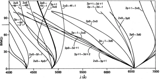
Wickramasinghe & Ferrario (2000) provide an extensive study of magnetic fields in all white dwarfs, finding that roughly 25 percent of all white dwarfs in cataclysmic variables have magnetic fields of at least 1 MG. The majority of magnetic cataclysmic variables with magnetic field strength measurements are between 1 and 60 MG, with only a handful of known stronger magnetic field strengths. Magnetic field measurements of white dwarfs in cataclysmic variables are made primarily through Zeeman splitting if the white dwarf pho-tosphere is visible or by the spacing of cyclotron harmonics. When available, the ratio of linear to circular polarization can also place a constraint on the magnetic field strength. It is important to note that the magnetic field strength measured through these different ways physically reflects the magnetic field strength at different locations.
Zeeman splitting most frequently is measured from the photosphere of the white dwarf. This splitting, which is uniform in frequency space, increases with magnetic field strength. The formerly single line has split into three components. In the linear Zeeman regime (for fields less than ∼20 MG), theπ component remains at the zero field frequency, and theσ+
this splitting can be approximated as
∆λL '4.7×10⁻⁷ λ2 Bs , (1.6.1)
whereλis in ˚A,Bsis the surface magnetic field in MG, and ∆λLis the separation of the split
components from the central component (Landstreet, 1980). At fields greater than∼20 MG the quadratic Zeeman effect begins to dominate, causing increasingly complicated structure in the line splittings. Figure 1.3 shows how for increasing field strengths, the line splittings get increasingly wider and more complicated. At any single instant, an observer is measuring the magnetic field strength averaged over the observed hemisphere and convolved with limb darkening. Disentangling this effect is difficult in white dwarfs that have multiple poles, and particularly in magnetic cataclysmic variables that might have multiple accreting poles at different field strengths. So frequently, magnetic field strengths from Zeeman splitting is a surface-averaged field strength, though serious effort has been made to carefully investigate the magnetic field structure on the white dwarf (Euchner et al., 2002).
Cyclotron radiation arises from the accretion shock region above the photosphere of the white dwarf. Individual electrons will radiate at frequencies based on
ωn =
n
(1−βkcosθ)
ωc
γ , (1.6.2)
where βk is the velocity component of the electron parallel to the magnetic field, γ = 1/p1−β2, and ω
c/γ is the fundamental cyclotron frequency (Bekefei, 1966).
Identify-ing successive harmonics can be used to estimate the magnetic field strength. The magnetic fields in polars are strong enough that the cyclotron humps can be shifted into the infrared or optical. If you have an identification of harmonic number, the field strength can be estimated by
λn =gn(Te)
10,700
n
108G
B
˚
A , (1.6.3)
where gn(Te) is approximately 1 for temperatures less than about 10 keV (Coyne et al.,
1988).
1.7 Plan for Measuring Properties of White Dwarfs in Binaries
1.8 Overview of Contents
In this dissertation, we present work measuring fundamental parameters of both single white dwarfs and those in attached binaries. For the white dwarfs in attached binaries, we have measured key parameters (mass, effective temperature, magnetic field strength) that have been measured accurately for only a few magnetic cataclysmic variables. For the single pulsating white dwarfs, we have determined Teff and logg of 122 white dwarfs from
spectroscopy. We have carefully limited and characterized the systematics involved in the determination of these parameters. The uniform calibration of Teff and logg will enable the
comparison to ensemble pulsation periods to examine relative structural differences in these stars. These values will also serve as important priors in the attempt to conduct absolute seismology of single, pulsating white dwarfs.
In chapter 2, we discuss the interesting magnetic cataclysmic variable LSQ1725-64. We discovered it in a low state of accretion, which allowed a measurement of the magnetic field strength and effective temperature of the white dwarf, as well as the spectral type of the secondary. Nightly monitoring with the PROMPT telescopes observed the transition from low accretion state to high accretion state to occur over a period of 3 days, placing an important constraint on the physical mechanism responsible for the different accretion states. Our precise timing measurements allow us to infer the mass of the white dwarf, which we find to be 0.966±0.027M. The unique geometry of LSQ1725-64 then permits an estimate of the mass transfer rate, and we find that no additional angular momentum loss mechanism besides gravitational radiation is required.
falling radially onto the white dwarf, it permits a measurement of the free-fall velocity very near the white dwarf surface.
In chapter 4, we will introduce and describe a large survey of pulsating DA white dwarfs that we have observed with the Goodman Spectrograph on the SOAR Telescope. This survey has produced the most systematically consistent set of DAV atmospheric parameters ever collected. We carefully characterize 10 systematics that can arise during the data reduction and fitting process and offer guidance and suggestions to future observers. We have found that flux calibration, extinction correction, or having models at different resolution than the observed spectrum can change the determined atmospheric parameters by up to 30 K and 0.01 dex in logg. Larger changes can come from changing the wavelengths at which lines are normalized (100 K and 0.02 dex) or night-to-night variations (51 K and 0.012 dex). We conclude by presenting Teff and logg for all 122 white dwarfs in the sample.
CHAPTER 2: THE MAGNETIC CATACLYSMIC VARIABLE LSQ1725-64 1
And so, with a graceful deportment and intrepidity, he settled
himself firm in his stirrups, grasped his lance, covered his breast
with his target, and posting himself in the midst of the highway,
stood waiting the coming up of those knights-errant; for such he
already judged them to be.
— Don Quixote
In this chapter, we present results of an investigation into the properties of the magnetic cataclysmic variable LSQ172554.8-643839 (hereafter LSQ1725-64). The results we present unambiguously classify LSQ1725-64 as a magnetic cataclysmic variable by estimating a mag-netic field strength of the white dwarf and the detection of multiple accretion states. We use high-speed photometry of the eclipse to estimate the mass of the white dwarf and spec-troscopy during a low accretion state to estimate the effective temperature of the white dwarf to provide two other fundamental parameters of the white dwarf in this system.
2.1 The Interesting Properties of Polar Candidate LSQ1725-64
LSQ1725-64 is an eclipsing binary with a period of∼94 minutes. Its V-band magnitude varies between 18 and>24 throughout the orbital cycle. It was first discovered as a variable star by Rabinowitz et al. (2011) as part of the La Silla-Quest Survey for Kuiper Belt Objects, stellar transients, and supernovae. Follow-up optical photometry showed an eclipse that lasted for ∼5 minutes with an ingress depth of more than 5.7 mag. Rabinowitz et al.
1The work presented in this chapter was originally published inMonthly Notices of the Royal Astronomical
(2011) noted that this is amongst the deepest eclipses known for all cataclysmic variables. They did not detect the star during eclipse in any optical band, but theirJ-band detection during eclipse provides some information about the secondary. However, without a color measurement they were only able to place a limit on the spectral class.
Rabinowitz et al. (2011) presented spectroscopy showing strong H and He emission, a radial velocity amplitude of 500km s−1, and Doppler broadening of 600-1300km s−1. These
observations led Rabinowitz et al. (2011) to suggest that LSQ1725-64 was a magnetic cat-aclysmic variable. However, the absence of strong He II or obvious cyclotron humps in the optical spectrum, the lack of prior X-ray or UV detections, and the absence of longterm mon-itoring or polarization data tempered the absolute classification of this system as a polar. Rabinowitz et al. (2011) therefore suggested follow-up time-resolved spectroscopy, photome-try with higher time resolution, longterm monitoring, polarization and other multiwavelength observations to confirm the classification of this object and study its properties
and Araujo-Betancor et al. 2005), or operates differently. Short period systems like LSQ1725-64 are particularly interesting to study, as there should be some period at which continued mass transfer causes the secondary to expand above its equilibrium radius, resulting in evolution to longer rather than shorter periods. The location of this period bounce and the evolution of systems that have passed through it are critical to our understanding of angular momentum loss and period evolution in cataclysmic variables.
Based on derived binary parameters and a V-J limit during eclipse, Rabinowitz et al. (2011) suggested LSQ1725-64 might be a post-bounce system, i.e. one that is already evolv-ing to longer orbital periods as the now degenerate secondary expands in response to mass loss. This would make it a rare and valuable object of study. These post-period-minimum systems have long been sought, with the first discovered by Littlefair et al. (2006). More have been found through the Sloan Digital Sky Survey (SDSS; see Littlefair et al. 2008 and G¨ansicke et al. 2009). In addition, LSQ1725-64 may offer the chance to explore the low accretion rate or low magnetic field strength regimes. On the basis of these interesting possi-bilities, we conducted a campaign of time-resolved spectroscopy, short cadence photometry, and photometric monitoring of LSQ1725-64.
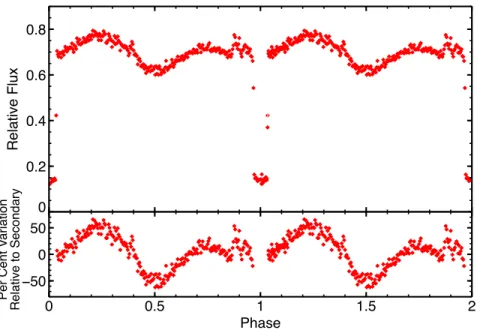
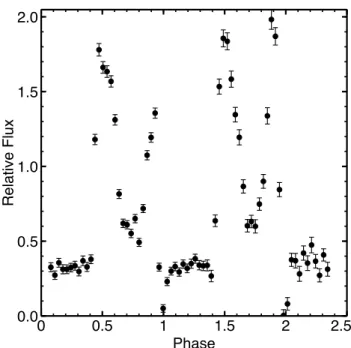
time-scales, we present typical high and low state lightcurves and interpret their features, relying on phenomena common to polars.
We have observed numerous eclipses of the white dwarf by the secondary, in both high and low states. During high state eclipse, the rapid ingress of the white dwarf is followed by a slower eclipse of very red light, presumably from optically thick gas in a loop above the accretion pole. The accretion pole is very near to the limb of the star at the moment of eclipse ingress. We interpret this light as coming from gas magnetically funneled by the magnetic field to the magnetic pole. We have used the measured height of this gas as a proxy for the Alfv´en radius.
In section 2.5, we present results from time-resolved optical spectroscopy. We do not see distinct cyclotron humps in the optical spectrum, but the color of the excess continuum during high state is too red to be thermal emission from a heated spot on the white dwarf. Rather it appears to be a smear of closely spaced cyclotron harmonics, such as seen in BL Hydri (Schwope et al., 1995), which has a similar magnetic field to LSQ1725-64. The trailed emission lines in our high state spectra show light dominated by recombination in the accretion stream, with little chromospheric activity from the secondary.
the line of centers. Our estimation of the Alfv´en radius allows us to infer an upper limit to the mass transfer rate of 6.1±3.4×10⁻¹¹M yr−1. This number is consistent with what we expect if gravitational radiation is the sole angular momentum loss mechanism. Finally, we conclude in section 2.7 by fitting LSQ1725-64 into context as a polar and adding our measurements to what is already known.
2.2 Observations
Our new observational data include three kinds of observations of LSQ1725-64: time-series spectroscopy, short cadence photometry, and photometric monitoring of accretion state.
As summarized in Table 2.1 and Table 2.2, we observed LSQ1725-64 on 14 separate nights with an imaging spectrograph—the Goodman Spectrograph on the 4.1-m SOAR Telescope. We obtained time-series photometry on 10 of those nights and time-series spectroscopy on 8 of those nights. On 4 nights we obtained both photometry and spectroscopy. The Goodman Spectrograph employs a 4k × 4k Fairchild 486 back-illuminated CCD with a plate scale of 0.15 arcsec pixel−1 (Clemens et al., 2004).
For the SOAR Goodman photometry, we binned the CCD at 2 × 2 with the exception of 2012-08-12, when we binned at 1 ×1. We did not use a filter for most of the photometry, allowing us to decrease the exposure times and increase the amount of time-dependent geo-metrical information in the data. For select eclipse measurements we obtained photometry in SDSS u0, g0, r0, and i0 bands. To reduce the readout time, the typical region of interest used was 90×90 arcsec, resulting in a readout time of∼3 s and a duty cycle greater than 80 per cent. All observations beginning in 2013 have GPS times recorded in the image header. Having accurate and believable timings is important for our determination of the ephemeris presented in subsection 2.4.1. Table 2.1 gives details of all our photometry.
Table 2.1: Photometric Observations with the Goodman Spectrograph on the SOAR Telescope and SALTICAM on SALT.
Observation Start Instrument Exposure Length of Eclipses Accretion
Date (UT) Time (s) Observation (hours) Observed State
2011-09-07 SALTICAM 15.7 1.8 1 High
2012-08-12 Goodman 20 4.5 3 High
2013-06-08 Goodman 20 1.7 1.5 Low
2013-07-03 Goodman 20 2.3 2 High
2013-07-06 SALTICAM 1.7 0.8 1 High
2013-07-12 Goodman 12 2.9 2 High
2013-07-27 Goodman 12 1.6 1 High
2013-08-05 Goodman 12 3.6 2 High
2013-08-14 Goodman 11 2.0 2 High
2013-08-15 Goodman 12 1.2 1 High
2013-09-02 SALTICAM 1.7 0.8 1 High
2013-11-14 Goodman 12 1.8 1 High
2014-06-30 Goodman 12 2.5 2 High
used a 1.6800 slit, but did not stay aligned to the parallactic angle. There was no Atmo-spheric Dispersion Corrector installed on the Goodman Spectrograph at the time of these observations. The resolution was set by the seeing and averaged ∼ 500 km s−1 at H α.
We took continuous sequences of spectra with no gaps, which limited the measurement of standards to only one a night. As a result of this observing strategy, our flux calibrations are less than ideal, but our velocity measurements, with errors∼40 km s−1, are as good as
the instrument can do given our resolution.
The Goodman Spectrograph employs Volume Phase Holographic gratings for use in spectroscopic mode. For nearly all observations, we used the 400 l mm−1 grating which provides a dispersion of 1 ˚A per unbinned pixel. Nearly all spectroscopic observations had exposure times of 300 s, equaling a phase width of 5.2 per cent. During eclipse, or low state, the typical signal-to-noise of the continuum from an individual spectrum was around 6 per binned pixel. In high state, the typical signal-to-noise of the continuum from an individual spectrum of the accreting hemisphere was between 8 and 13 per binned pixel.
Table 2.2: Spectroscopic Observations with the Goodman Spectrograph
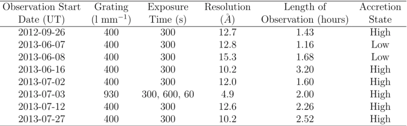
Observation Start Grating Exposure Resolution Length of Accretion Date (UT) (l mm−1) Time (s) (˚A) Observation (hours) State
2012-09-26 400 300 12.7 1.43 High
2013-06-07 400 300 12.8 1.16 Low
2013-06-08 400 300 15.3 1.68 Low
2013-06-16 400 300 10.2 3.20 High
2013-07-02 400 300 12.0 1.60 High
2013-07-03 930 300, 600, 60 4.9 2.00 High
2013-07-12 400 300 12.6 2.26 High
2013-07-27 400 300 10.2 2.52 High
the flux changes at different timescales throughout the orbit. Table 2.2 gives details of all our spectroscopy.
We also observed LSQ1725-64 three times with the SALTICAM Imager on the South-ern African Large Telescope (O’Donoghue et al., 2006). We used frame transfer mode on SALTICAM, which allows half the chip to be shifted onto the unexposed half of the chip nearly instantaneously, limiting dead time between exposures. The first observation with SALT was taken in September 2011. The exposure time for these data were 15.7 s. Two more observations were taken in dark time with SALT in 2013 with exposure times of 1.7 s. As with the Goodman photometry, we did not use a filter. The observations with SALT did not cover a full orbit, but instead were centered on the eclipse to resolve the ingress and egress structure.
We also used the PROMPT network of robotic telescopes to monitor the accretion state of LSQ1725-64. As with the other photometry, we did not use a filter. PROMPT has primary mirrors of 0.41-m, so longer exposures were needed to detect LSQ1725-64. Exposure times were 180 s, with a readout time of ∼6 s, providing a duty cycle of 96.7 per cent. PROMPT monitored LSQ1725-64 on 70 separate nights during low, high, and intermediate states. We typically obtained one orbit per night.
interference patterns. Lightcurves were produced using APER, an IDL function based on DAOPHOT (Stetson, 1987). All photometry makes use of the same three nearby comparison stars. To correct for longterm environmental trends in the lightcurve, we divided the flux from LSQ1725-64 by the average flux from the three comparison stars. We then define the mean flux as the average in region 2 on the night of 2013-07-02. All photometry is presented relative to this average.
Spectroscopic observations were bias subtracted but were also not flat-fielded. The thinned CCD on Goodman leads to fringing effects at wavelengths longer than 6000 ˚A that make flat-fielding an imprecise task. The spectra were extracted and wavelength calibrated using the standard IRAF tasks and a HgAr lamp. We produced rough flux calibrations by measuring the instrument response with a standard star. We did not sample the same range of airmasses in these standards as in the data, so the main sources of error in the flux calibration are changes in extinction and differential slit losses.
2.3 The Magnetic Field of the White Dwarf
There are three primary ways to measure the magnetic field strength of the white dwarf in accreting binary systems: the ratio of circular to linear polarization (Meggitt & Wickramas-inghe, 1982), the presence and spacing of cyclotron humps in phased-resolved spectroscopy (Wickramasinghe & Ferrario, 2000), or the fitting of Zeeman splitting in absorption lines when the system enters a low state and the photosphere of the white dwarf becomes vis-ible (e.g. Schwope et al. 1993). No distinct, identifiable cyclotron humps are observed in our time-resolved spectra, and we do not have polarization measurements; however the ob-served low state in LSQ1725-64 allowed us to measure the Zeeman splitting of H β in our spectroscopic observations.
Zeeman effect is calculable by
∆λL '4.7×10⁻⁷ λ2 Bs , (2.3.1)
where λ is in ˚A, Bs is the surface magnetic field in MG, and ∆λL is the separation of the
split components from the central component (Landstreet, 1980).
Figure 2.1: Orbital-averaged low state spectrum of LSQ1725-64 showing Zeeman splitting of the H β line. The fit to determine the splitting is shown in red. The best-fitting model indicates a surface-averaged magnetic field of 12.5 ± 0.5 MG, consistent with white dwarf magnetic field strengths expected in polars.
From Equation 3.6.1 we determine a surface-averaged magnetic field of 12.5 ± 0.5 MG. This magnetic field strength of the white dwarf falls within what is expected for polars. The field strength at which no accretion disk can form is believed to begin around 10 MG, though this depends on the accretion rate. The polar V2301 Oph has the lowest known field strength of 7 MG (Ferrario et al., 1995). The absence of distinct cyclotron humps is not in conflict with the field strength we have measured. We will show in section 2.5 that the spectrum during high state is very similar to that seen in BL Hydri (Schwope et al., 1995), which also has a measured field strength of 12 MG. Like LSQ1725-64, BL Hydri does not show distinct cyclotron humps in high state but rather a single broad hump peaking at 7500 ˚
A. Schwope et al. (1995) attribute this to several closely spaced and overlapping cyclotron harmonics that merge together to form a single hump. The same explanation plausibly explains our data, but makes it impossible to estimate the magnetic field strength from the spacing of cyclotron harmonics. Consequently, our measurement of Zeeman splitting offers the best confirmation that the white dwarf in LSQ1725-64 has a strong magnetic field, and allows definitive classification of the binary as a cataclysmic variable of the AM Her type.
2.4 Photometric Properties of LSQ1725-64
In this section we will present and discuss photometric data gathered on time-scales ranging from seconds to months. We begin with the periodic variations that repeat or almost repeat in each orbital cycle and are best studied using light curves folded at the orbital period. Then we present the longer time-scale state changes related to the accretion cycles of the binary. Both of these analyses require that we first update the orbital ephemeris of the binary.
2.4.1 Orbital Ephemeris
when the polar was in a high state. In this state the eclipse ingress is preceded by flickering and includes both the eclipse of the white dwarf and of the accreting pole, which is very near to the limb. This makes it difficult to measure the time of mid-ingress. The eclipse egress does not show this behavior and lasts 23.4 ± 0.3 s. Thus we measured eclipse times for all of our photometric data using times of mid-egress. The measured mid-egress times were all adjusted to Barycentric Julian Date in the Barycentric Dynamical Time standard (BJ DT DB) using the code of Eastman et al. (2010). Only SOAR and SALT eclipse data
were used to calculate the ephemeris, the time resolution from PROMPT data is not good enough to measure the mid-egress time.
Figure 2.2: A SALT lightcurve of LSQ1725-64 from 2013-07-06 with an exposure time of 1.7 s. The structure of the eclipse ingress of the white dwarf and hotspot is not resolved with this time sampling. The egress of the white dwarf lasts 23.4± 0.3 s and appears unaffected by any hotspot.