THE GEOMETRY OF RADIAL STATES IN NONLINEAR ELLIPTIC PROBLEMS
Bevin Laurel Maultsby
A dissertation submitted to the faculty at the University of North Carolina at Chapel Hill in partial fulfillment of the requirements for the degree of Doctor of Philosophy in the
Department of Mathematics.
Chapel Hill 2014
Approved by:
Christopher K.R.T. Jones Graham Cox
c 2014
ABSTRACT
Bevin Laurel Maultsby: The Geometry of Radial States in Nonlinear Elliptic Problems
(Under the direction of Christopher K.R.T. Jones)
In this dissertation we present a geometric approach to the study of nonlinear elliptic problems. In particular, we analyze radial solutions using techniques from dynamical systems. These techniques include a thorough study of the invariant manifolds that arise from the union of the solutions to the elliptic PDE in phase space, as well as computations involving two vector fields which are tangent to the invariant manifolds.
In Chapter 3, we consider radially symmetric positive solutions to ∆pu+f(u) = 0 on a ball centered at the origin in Rn. The union of all radially symmetric solutions to this quasilinear elliptic equation forms an invariant manifold. We use two integral expressions that arise from vector fields on the manifold to show that for a certain class of f, there can be at most one such solution satisfying ∆pu+f(u) = 0 on a ball with Dirichlet boundary conditions.
In Chapter 4, we make a powerful connection between the Morse index of the operator
ACKNOWLEDGEMENTS
I began my mathematics career at UNC as an undergraduate math major; I am thus grateful not only to the mathematics faculty I worked with as a graduate student, but also to those professors whose classes originally inspired me to apply to graduate school. I am grateful to my advisor, Dr. Christopher K.R.T. Jones, for his constant encouragement and support, not only mathematically but also personally. Special thanks as well are due to Jeremy Marzuola as the person who motivated much of this work. I also would like to thank Graham Cox for a lot of feedback and for pointing out to me the work of Francesca Dalbono; her work with Franca on the existence of solutions to ∆pu+f(u) = 0 inspired me to investigate conditions for uniqueness. I would also like to thank Patrick Eberlein and Jason Metcalfe for their service and feedback on my committee as well as for their excellent teaching in geometry and analysis.
TABLE OF CONTENTS
LIST OF FIGURES . . . viii
CHAPTER 1: INTRODUCTION . . . 1
1.1 Overview . . . 1
1.2 Dynamical systems . . . 2
1.2.1 Basic definitions . . . 2
1.2.2 Invariant manifolds . . . 3
1.2.3 A review of the variational equation in differential form notation . . . 6
1.3 Elliptic equations . . . 8
1.3.1 Sobolev Spaces . . . 10
1.4 Sturm-Liouville Theory . . . 11
1.5 Applications . . . 16
1.6 Overview of dissertation . . . 16
CHAPTER 2: BACKGROUND . . . 17
2.1 Results on uniformly elliptic partial differential equations . . . 17
2.2 Results for the p-Laplacian . . . 20
CHAPTER 3: UNIQUENESS OF POSITIVE SOLUTIONS FOR THE p-LAPLACIAN, 1< p <2 . . . 23
3.1 Set-up as a dynamical system . . . 26
3.1.1 Dynamical system in (u, ω, r)-coordinates . . . 27
3.1.2 Dynamical system in (y, w, r)-coordinates . . . 30
3.2 Critical exponents and existence of solutions . . . 33
3.2.1 Wpu,c under the Emden–Fowler transformation . . . 34
3.2.2 Existence of solutions . . . 35
3.3.1 Definitions . . . 37
3.3.2 Variational equations . . . 39
3.4 Proof of uniqueness . . . 47
3.4.1 Eliminate Underrotation . . . 56
3.4.2 The overrotation cases . . . 56
3.4.3 Proof for Case (1) (the asymptote case) . . . 59
3.4.4 Proof for Case (2) . . . 60
3.4.5 Proof for Case (3) . . . 61
3.5 Summary . . . 63
CHAPTER 4: MORSE INDICES OF SIGN-CHANGING SOLUTIONS . . . 65
4.1 Statement of theorems . . . 66
4.2 Morse index . . . 68
4.3 Sturm-Liouville theory . . . 69
4.4 Proofs of results on δu, 1< p≤2 . . . 74
4.5 Proofs of theorems on the Morse index of ∆u+f(u) = 0 . . . 82
4.6 Proof of Theorem 4.6.1 . . . 83
CHAPTER 5: REMARKS AND FUTURE DIRECTIONS . . . 94
5.1 Hyperbolic metric . . . 94
5.2 Algal bloom model . . . 96
LIST OF FIGURES
1.1 Oscillatory behavior of eigenfunctions to a Sturm-Liouville system . . . 15
3.1 The invariant manifolds for radial solutions to (3.13)-(3.15). . . 29
3.2 The invariant manifolds of (y, w, r) = (0,0,0) in the {r= 0} plane. . . 37
3.3 The effect of choosingq1 < p∗, q1 =p∗, and q1 > p∗ in the plane {r= 0}. . . 38
3.4 The curves γ =γ(ˆτ ,αˆ) and C(ˆτ ,αˆ). . . 41
3.5 An illustration ofI(cτ(a)). . . 43
3.6 An imagined Sγ(τ,α) from Lemma 3.3.1 satisfying ˙δu = 1/(p−1)|ω| 2−p p−1. . . . 44
3.7 The overrotation setup for Lemma 3.4.1. . . 49
3.8 The general form of C(τ,αˆ) in Lemma 3.4.1 with underrotation. . . 50
3.9 The general form of C(τ,αˆ) in Lemma 3.4.1 with overrotation. . . 51
3.10 A plot of K(u0)−K(u),f(u), and the product (K(u0)−K(u))f(u). . . 57
3.11 The graph of Λ(u) from (3.72) . . . 58
4.1 The oscillatory behavior of δu compared to the eigenfunctions of (4.7). . . . 71
4.2 The curve C(tk, αk) in the plane {r =r(tk)} described in Corollary 4.4.7. . . 80
4.3 The six possible subcases of Case A in the proof of Theorem 4.6.1. . . 88
4.4 The six possible subcases of Case B in the proof of Theorem 4.6.1. . . 89
4.5 Six of the possible twelve subcases of Case C in the proof of Theorem 4.6.1. . 90
4.6 The other six possible subcases of Case C in the proof of Theorem 4.6.1. . . 91
4.7 Six of the possible twelve subcases of Case D in the proof of Theorem 4.6.1. . 92
CHAPTER 1: INTRODUCTION
1.1 Overview
The goal of this dissertation is to study nonlinear elliptic PDEs by using techniques from geometric dynamical systems. Of particular interest is the p-Laplacian operator ∆p, which may be singular or nondegenerate and which arises as an Euler-Lagrange equation to a Dirichlet integral.
In the 1980’s, a great deal was discovered about positive solutions to semilinear elliptic equations of the form ∆u+ f(u) = 0 on a selected domain with appropriate boundary conditions; we will focus on a ball of radius |x| = R centered at the origin with Dirichlet boundary conditions. Kwong [22] proved that positive radial solutions of such an elliptic PDE on this domain were unique provided f(u) was of a certain “superlinear” form; his results were extended by McLeod [25] to different f(u). In Clemons’ 1990 dissertation under Jones, he constructed a geometric argument for uniqueness of positive solutions satisfying ∆u+f(u) = 0 on this domain by studying the invariant manifold created by the relevant radial solutions; see [7].
Our starting goal was to show uniqueness of sign-changing solutions to ∆u+f(u) = 0 on a ball with Dirichlet boundary conditions. The question was: if uhas k zeros onBR(0), is it necessarily unique (perhaps with a small radius R)? In pursuit of this question, we supplemented the vector field that was used by Clemons and Jones [7] to show uniqueness in the case k = 1 in with another vector field whose geometry can be tracked asu changes signs and |x| →R. Although the original question remains open, we were able to provide results on the Morse index of a sign-changing solution to ∆u+f(u) = 0. This material is the subject of Chapter 4.
-Laplacian is its quasilinear counterpart. Thep-Laplace equation ∆pu+f(u) = 0 is challenging as the p-Laplacian is non-uniformly elliptic if p 6= 2 and singular if p ∈ (1,2). Using two vector fields along solutions to ∆pu+f(u) = 0 in the ball BR(0), we prove that a positive radial solution satisfying a Dirichlet boundary condition must be unique. Most of Chapter 3 is dedicated to this proof.
In the rest of this introductory chapter, we provide the necessary background information to understand key concepts from dynamical systems and elliptic partial differential equations that will be used in subsequent chapters. The introduction concludes with a summary of Chapters 2-4.
1.2 Dynamical systems
Let us begin with a basic definition of a dynamical system, the flow it generates, and interesting structures that may arise; much of this material follows [33].
1.2.1 Basic definitions
Definition 1.2.1. A dynamical systemis a smooth manifold (called the phase space) U
endowed with a family of smooth functions Φ(x, t) : Ω ⊂U ×I →U, where I ⊂R. Setting Φt(x) = Φ(x, t), the Φt satisfy
• Φ0(x) = x, for all x∈U, and
• Φt◦Φs(x) = Φt+s(x), if both sides are defined.
The group of functions Φt(x) is called a flow on U, and it evolves each point inU by time
t ∈ I. Generally speaking, a dynamical system is a space U together with a rule for how points in that space evolve. This rule generates a vector field F :U ⊂Rn →
Rn in phase space; for an autonomous dynamical system, the vector field is often written
˙
x=F(x), (1.1)
p∈U is acritical point (or fixed point) of (1.1) if F(p) = 0. Consequently Φ(p, t) =p for any t∈I.
1.2.2 Invariant manifolds
Invariant manifolds are special types of invariant sets for (1.1). While they may arise in relation to, say, a periodic orbit, we will focus below on invariant manifolds of a fixed point p∈U. As the name suggests, an invariant manifold is “invariant” under the flow Φ, where we define invariant sets using the following definition.
Definition 1.2.2. A setB ⊂U is positively invariantif B ·t⊂B for all t≥0, where
B·t={Φt(x)|x∈B}.
B is negatively invariant if B·t ⊂ B for all t ≤ 0. We say B is invariant if it is both positively and negatively invariant.
Basic examples of invariant sets in phase space include critical points, periodic orbits, and regions trapped by homoclinic orbits.
To construct an invariant manifold, we begin by linearizing the system (1.1) at a critical point. In particular, suppose U ⊂ Rn is open, and consider a C1 vector field F(x) for all
x∈U. Let p∈U be a critical point; the linearization of (1.1) at pis
˙
y=DF(p)y (1.2)
where y∈Rn andDF(p) is an n×n matrix. To study the eigenvalues of DF(p), let σ(∗) denote the spectrum of∗. The set of eigenvalues of DF(p) decomposes into subsets via
σ(DF(p)) =σ−∪σ0∪σ+
Reλ = 0 and σ+ to eigenvalues with Reλ > 0. Furthermore, the matrix DF(p) can be
diagonalized to the block form
DF(p) =
A− 0 0
0 A0 0
0 0 A+
with σ(A−) = σ−, etc. Spanned by each set of eigenvalues σ−, σ0, and σ+ of DF(p) are
invariant subspaces E−, E0, andE+ such that
Rn =E−⊕E0⊕E+
and
σ(DF(p)|E−) = σ−, etc.
Each subspace E−, E0, and E+ is an invariant set for (1.2), which is a linear dynamical system.
With each of the subspaces E−, E0, E+ established, we define the invariant manifolds.
These manifolds give a “nonlinear” version of the invariant subspaces. There are three classes of invariant manifolds: stable manifolds, unstable manifolds, and center manifolds, which are analogous to E−,E+, and E0, respectively. Let N be an open neighborhood of the fixed
point p; the stable manifold is (locally) characterized as follows:
Definition 1.2.3. The local stable manifold is
Wlocs (p) ={x∈N |x·t ∈N for all t≥0,x·t→p exponentially as t → ∞}. (1.3)
tend exponentially towards p ast → ∞. Analogously, thelocal unstable manifold is the set
Wlocu (p) = {x∈N |x·t∈N for all t≤0,x·t→p exponentially as t→ −∞} (1.4)
so that the local unstable manifold consists of all points which evolve to p as time is reversed. Notice both local manifolds are nonempty, as they both contain p.
Theorem 1.2.4 (Stable and Unstable Manifold Theorem). Assume F ∈C1 and pis
a fixed point. Then there is a neighborhood N of p and a Lipschitz function
hs : (p+E−)∩N →E0⊕E+
so that the graph of hs is Ws
loc. There exists also a neighborhood M of p and a Lipschitz
function
hu : (p+E+)∩M →E−⊕E0
so that the graph of hu is Wlocu .
This theorem justifies calling the local stable and unstable manifolds defined in (1.3)-(1.4)“manifolds,” as they are the graphs of Lipschitz functions.
Both local manifolds extend into global invariant manifolds. With U ⊂Rn as before and for any choice of neighborhood N, the global versions are constructed by evolving Ws
loc(p)
and Wu
loc(p) backwards and forwards in time, respectively.
Definition 1.2.5. The (global) stable manifoldis
Ws(p) ={Φt(x)|x∈Wlocs (p), t≤0}. (1.5)
Similarly, the (global) unstable manifold is defined as
As discussed in [33], the stable and unstable manifolds are unique, and their tangent spaces atp are E− and E+, respectively.
A fixed pointpishyperbolicif the real part of each eigenvalueλ ∈σ(DF(p)) is nonzero. If p is not hyperbolic, then the center subspaceE0 is nontrivial. Associated withE0 is the idea
of a center manifold whose tangent space atp isE0. For a neighborhoodN 3p, trajectories
that stay in N for all t ≥0 tend to the center manifold as t → ∞, while trajectories that stay in N for all t≤0 tend to the center manifold as t→ −∞.
We note that global stable and unstable manifolds are always unique, but center manifolds are not necessarily so. In general, center manifolds are more difficult to define precisely than stable and unstable manifolds, and the reader should consult [33].
1.2.3 A review of the variational equation in differential form notation
To increase readability, we switch the notation in this section from ˙xto x0. Consider an autonomous dynamical system
x0 =F(x), x∈U ⊂Rn
as before. If x(t) is a solution to x0 = F(x), andδ0 is a vector tangent to x(t) at t= t0, then δ0 satisfies the variational equation
δ0 =DF(x)δ. (1.7)
This equation generates a tangent vector field δ(t) with δ(t0) =δ0 and describes how these
tangent vectors move under the flow. As DF(x) is an n×n matrix andδ is an n×1 vector, the ith coordinate of δ0 is
δi0 = (dxi(δ))0 = n X
j=1
We suppress the tangent vector δ and write
dxi0 = n X
j=1
∂jFi(x)dxj.
However, it should be understood that dxi0 applies to a tangent vector. This calculation establishes what it means to take the derivative of a 1-form.
Consider now a 2-form dzi ∧dzj applied to a pair of vectors (δ1, δ2). We claim that
(dzi ∧dzj)0, where the idea of a “derivative of a form” is the same as above, follows the product rule. To show this, we perform the following steps:
(dzi∧dzj)
0
= [dzi∧dzj(δ1, δ2)] 0
= d
dt [dzi(δ1)dzj(δ2)−dzi(δ2)dzj(δ1)]
= dzi(δ1)0dzj(δ2) +dzi(δ1)dzj(δ2)0−dzi(δ2)0dzj(δ1)−dzi(δ2)dzj(δ1)0
= dzi(δ1)0dzj(δ2)−dzi(δ2)0dzj(δ1) +dzi(δ1)dzj(δ2)0 −dzi(δ2)dzj(δ1)0
= dzi0∧dzj +dzi∧dzj0. (1.8)
In other words, if we construct a function of t given by
ω(t) = du∧dv(δ1(t), δ2(t)),
then using the product rule above yields
ω0(t) = d
dt[du∧dv(δ1(t), δ2(t))]
= · · ·
= (du∧dv)0(δ1(t), δ2(t)),
Suppose that for a given dynamical system in R3 described by x0 = F(x), where x =
(y, w, r)T, we have two linearly independent vector fields (y0, w0, r0)T and (δy, δw, δr)T that are tangent to an invariant manifold. (The notation is relevant to Chapters 3-4, and rather than define these vector fields here we will simply assume that they are linearly independent as described.) As they are tangent vector fields, both satisfy (1.7). Their cross-product,
(δy∗, δw∗, δr∗)T := ( ˙y,w,˙ r˙)T ×(δy, δw, δr)T,
is a vector field normal to the invariant manifold, and it satisfies the following lemma.
Lemma 1.2.6. For a dynamical system x0 =F(x), let A=DF(x) and let (δy∗, δw∗, δr∗)T
be defined as above. Then this normal vector satisfies
δy∗ δw∗ δr∗ 0
= (−A∗+ (TrA)I) δy∗ δw∗ δr∗ ,
where A∗ is the transpose of A.
The proof is a straightforward matrix calculation. Lemma 1.2.6 will be consistently employed to easily compute time derivatives of 2-forms in Chapters 3 and 4.
1.3 Elliptic equations
We first recall some of the elementary definitions and results for elliptic partial differential equations and Sobolev spaces; see [14] and [32]. Through this section Ω⊂Rn is a bounded domain (an open connected set) with smooth boundary∂Ω, andu: Ω→Ris inC2(Ω)∩C(Ω). We remark that for Chapters 2-4, Ω will be the open ball
BR(0) ={x∈Rn | |x|< R}, n ≥2.
operator L given by
Lu:= n X
i,j=1
aij(x)uxixj +
n X
i=1
bi(x)uxi +c(x)u (1.9)
is elliptic if there is some constant θ >0 such that
n X
i,j=1
aij(x)ξiξj ≥θ|ξ|2, (1.10)
for a.e. x∈Ω and all ξ∈Rn.
In Chapter 2-4, we will consider quasilinear elliptic equations with the following second order operator.
Definition 1.3.2. The p-Laplacian ∆p is defined by
∆pu= div |∇u|p
−2
∇u, (1.11)
where u: Ω⊂Rn → R.
When p= 2, ∆p is the regular uniformly-elliptic Laplacian. When 1< p <2, (1.11) is a singular operator, as it is undefined whenever ∇u= 0. Wheneverp > 2, ∆p is a degenerate elliptic operator; in other words, ∆p satisfies (1.10) with the weaker condition obtained by setting θ= 0.
Note setting (1.11) equal to zero is the Euler-Lagrange equation for the Dirichlet integral
J(u) = Z
Ω
|∇u|pdx.
extensions. For an in-depth treatise of the p-Laplacian andp-harmonic functions, we advise the reader to consult [24].
The general form of the nonlinear elliptic problems studied in Chapters 2-4 is
∆pu+f(u) = 0 onBR(0)
u = 0 on∂BR(0),
(1.12)
where p∈(1,2] and f(u) is a nonlinear function. 1.3.1 Sobolev Spaces
The solutions to the elliptic equations such as (1.12) live naturally in Sobolev spaces. Let Ω⊂Rn be a domain. The Sobolev spaceW1,p
0 (Ω) is the completion of C0∞(Ω) with respect
to the norm
||u||p
W01,p(Ω) =
Z
Ω
(|∇u|p+|u|p) dx. (1.13)
Thus, W01,p(Ω) is a Banach space. In the casep= 2, W01,2(Ω) is a Hilbert space with inner product
hu, viW1,2 0 (Ω) =
Z
Ω
(∇u· ∇v+uv) dx.
Consider the energy functional
Jp(u) = 1
p
Z
Ω
|∇u|pdx− Z
Ω
F(u(x))dx, (1.14)
where F(t) = R0tf(s)ds for a function f ∈ C1([0,∞)). Critical points minimizing the
functional must satisfy
Z
Ω
|∇u|p−2∇
u· ∇φ−f(u)φ
dx= 0,
the equation
∆pu+f(u) = 0,
with Dirichlet boundary conditions.
Definition 1.3.3. For the Sobolev space W1,p(Ω), Ω⊂
Rn, the Sobolev critical exponent is defined by
1
p∗ :=
1
p −
1
n. (1.15)
Hence p∗ =np/(n−p). The importance of (1.15) is that as we investigate equations of the form ∆pu+f(u) = 0, we choose nonlinearities f(u) with the “correct” growth|u|q−2u.
In particular, we will choose the exponent term q so that q satisfies case (2) in the following theorem.
Theorem 1.3.4 (Sobolev, Rellich, Kondrachov). If 1< p < n, then
1. W1,p(Ω),→Lp∗(Ω) is a continuous embedding, and
2. if q < p∗+ 1, W1,p(Ω),→Lq−1(Ω) is a compact embedding.
Notice that the hypothesis 1< p < nis easily satisfied if p∈(1,2) and n≥2. 1.4 Sturm-Liouville Theory
A Sturm-Liouville (SL) equation is a type of ordinary differential equation in a finite domain with a well-understood set of eigenvalues and eigenfunctions. In particular, its eigenvalues are always real and discrete. Typically SL equations are described as having a smallest eigenvalue, from which the eigenvalues increase without bound. We shall cast SL equations slightly differently so that the eigenvalues have a largest member and decrease without limit; this change is convenient in the language of dynamical systems as positive eigenvalues are unstable.
results is that once we have identified a particular ODE as an SL system, then the results on eigenvalues and eigenfunctions described in this section are immediately applicable to the system.
We will state most of the major theorems on SL equations to provide the necessary background for Chapter 4; this presentation of SL equations follows [5]. Most sources, including [5], use Green’s formula to prove the theorems in this section; we use a slight variation on the usual techniques.
An SL differential equation is of the form
(f1(x)u0(x)) 0
+f2(x)u(x) =λf3(x)u(x), (1.16)
where each fi(x) is real and continuous, f10(x) is continuous, and f1(x) and f3(x) are positive
on the open interval (a, b). This type of equation can be viewed as an eigenvalue problem for the linear operator L defined by
L:u(x)7→(f1(x)u0(x)) 0
+f2(x)u(x). (1.17)
The boundary conditions for the types of regular SL systems we consider are either Dirichlet, Neumann, or Robin conditions at a and b. These conditions can be written
(1) α1u(a) +α2u0(a) = 0, and
(2) β1u(b) +β2u0(b) = 0,
(1.18)
where αi, βi ∈ R, with α21 +α22 >0, β12 +β22 >0. A eigenfunction solution uλ(x) to (1.16) corresponding to eigenvalue λ is regular if uλ(x)∈C1([a, b]).
Let us establish a series of basic results about SL equations which we will use in Chapter 4.
Proof. Suppose λ is an eigenvalue with eigenfunctions u1 6=u2. To examine u1 andu2, let us
compute the Wronskian of u1 and u2 at the left endpointx=a:
W(u1, u2)(a) =
u1 u2
u01 u02
x=a
=u1(a)u02(a)−u 0
1(a)u2(a) = 0, (1.19)
by (1.21). Thus the two columns are proportional, and we may say u2(a) = Cu1(a). By
Abel’s identity for second-order ordinary differential equations, for any c∈[a, b],
W(u1, u2)(c) =
u1 u2
u01 u02
x=c
=W(u1, u2)(a)e−
Rc af
0
1(s)/f1(s)ds = 0.
As f1(x) > 0 for a ≤ x ≤ b, the above expression is defined. Hence the columns are
proportional for any x ∈ [a, b], and so u2(x) = Cu1(x). Thus the eigenspace for λ is
1-dimensional.
The function f3(x) gives rise to the following inner product:
uλi(x), uλj(x)
=
Z b a
f3(x)uλi(x)uλj(x)dx. (1.20)
Theorem 1.4.2. If i6=j, then uλi(x) and uλj(x) are orthogonal with respect to (1.20).
Proof. First, we claim that at either endpoint x=a or x=b,
u0λ
iuλj|a=uλiu
0
λj|a, u
0
λiuλj|b =uλiu
0
λj|b. (1.21)
The equalities in (1.21) stem from the mixed linear boundary conditions; if αi, βi 6= 0, then
u0λ
i(b)uλj(b) = −
β1 β2
uλi(b)
−β2
β1 u0λ
j(b)
=uλi(b)u
0
λj(b),
uλi(b)u
0
λj(b).
Assume without loss of generality that λi 6= 0 (in which case it may be possible for λj to be zero). Using the above statement and integration by parts, we obtain
uλi, uλj
=
Z b a
f3(x)uλiuλjdx
= 1
λi Z b
a
λif3(x)uλiuλjdx
= 1
λi Z b
a
uλj f1(x)u
0 λi 0 dx+ Z b a
f2(x)uλiuλjdx
= 1
λi
uλjf1(x)u
0
λi|
b a−
Z b a
u0λ
jf1(x)u
0
λidx+
Z b a
f2(x)uλiuλjdx
.
By (1.21), we can write this as
= 1
λi
uλif1(x)u
0
λj|
b a−
Z b a
u0λ
if1(x)u
0
λjdx+
Z b a
f2(x)uλiuλjdx
= 1
λi Z b
a
uλi
f1(x)u0λj
0
dx+ Z b
a
f2(x)uλiuλjdx
= 1
λi Z b
a
f3(x)uλiLuλjdx
= λj
λi Z b
a
f3(x)uλiuλjdx
= λj
λi
uλi, uλj
.
If λi 6=λj, then for the above conclusion to hold, it must be the case that
uλi, uλj
= 0.
Theorem 1.4.3. The eigenvalues of a regular SL system are real.
Proof. Letu be a nondegenerate eigenfunction which solves (1.16) with eigenvalue λ. Then
u solves (1.16) with eigenvalueλ. As 0∈R, assumeλ 6= 0. From the proof of Theorem 1.4.2, we know
1 1
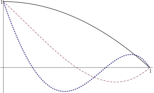
Figure 1.1: An illustration of the general oscillatory behavior of the first three eigenfunctions to a SL problem, with boundary conditions u(0) = 1 and u(1) = 0. In this picture, the solid line represents the eigenfunction uλ0, the dashed line uλ1 and the dotted line uλ2.
Yet in order for this to be true, we must have λ=λ. So λ∈R.
By Theorem 1.4.1, eigenfunctions of an SL system are unique up to scalar multiplication. Therefore, together with Theorem 1.4.2, we can normalize the eigenfunctions to form an orthonormal set.
Theorem 1.4.4 (Sturm Comparison Theorem). Let λi and λj be two eigenvalues with
eigenfunctions uλi and uλj satisfying (1.16). If λi > λj, then between consecutive zeros of
uλi, there lies at least one zero of uλj .
We omit the proof of Theorem 1.4.4, as it is very similar to the proof of Lemma 4.3.1 in Chapter 4. We will also omit the proof of the following theorem, as it is a standard result:
Theorem 1.4.5. The SL problem (1.16) with regular boundary conditions (1.18) has an infinite set of real eigenvalues
λ0 > λ1 > λ2 >· · · with lim
and therefore an infinite number of eigenfunctions uλn(x). Moreover, each eigenfunction
uλn(x) is unique (up to scalar multiplication) and has exactly n zeros on the open interval
(a, b).
The consequences of Theorems 1.4.4 and 1.4.5 on the behavior of eigenfunctions is illustrated in Figure 1.1. In this illustration, the eigenfunction uλ0 has 0 zeros in (0,1), uλ1 has 1 zero in (0,1), anduλ2 has 2 zeros in (0,1).
1.5 Applications
Let us conclude the introduction by mentioning one of the major applications of the
p-Laplacian. In particular, we remark that the regular Laplacian ∆uis a model for Newtonian fluids, which are characterized by having the viscous stress proportional to the strain rate at every point; see, e.g., [4]. The factor |∇u|p−2 describes the speed that fluid particles travel
in relation to each other; this term reduces to 1 in the linear Newtonian setting. For a non-Newtonian fluid, |∇u|p−2 relates the effect of shear on the viscosity of the fluid. Hence
the p-Laplacian ∆p may be used to model non-Newtonian fluids.
In particular, 1< p <2 models pseudoplastics, which are fluids that become less viscous as the shear increases (examples include blood, several types of paint, nail polish). The case p >2 models dilatants, which become more viscous as the shear increases (the classic example is cornstarch in water).
1.6 Overview of dissertation
CHAPTER 2: BACKGROUND
In this chapter we give an overview of the history and previous results on the semilinear elliptic equation
∆u+f(u) = 0, (2.1)
and the quasilinear elliptic equation
∆pu+f(u) = 0, (2.2)
for different classes of nonlinearities f and in various domains with appropriate boundary conditions.
2.1 Results on uniformly elliptic partial differential equations
In this section we discuss the symmetry of positive solutions to (2.1), where the domain is typically a ball with Dirichlet boundary conditions, as well as results on existence and uniqueness for solutions to (2.1).
With the technique of moving parallel planes, Serrin showed in [30] that if Ω is a smooth bounded domain and u is a positive solution to ∆u+ 1 = 0 in Ω, withu= 0 on ∂Ω and with the outward normal vector ∂u∂ν constant on ∂Ω, then Ω is necessarily a ball and u is a radial function. The method of moving parallel planes was originally used by Alexandroff to study surfaces of constant mean curvature in differential geometry. It was also used by Gidas, Ni and Nirenberg [18] to obtain the following famous result.
Theorem 2.1.1 (Gidas, Ni, Nirenberg). In the ball Ω ={x∈Rn | |x|< R}, let u >0 be a
positive solution in C2( ¯Ω) of
Here f is of class C1. Then u is radially symmetric and
∂u
∂r <0, for 0< r < R.
Part of the power of this result stems from the fact that they make no assumptions on the nonlinear term f(u) except thatf ∈C1.
In general, existence and uniqueness results for (2.1) and (2.2) do require more restrictive conditions on f(u). The prototypical example is the Lane-Emden equation f(u) = uq, for
q >1. Ifq = (n+ 2)/(n−2) = 2∗−1, where 2∗ is the Sobolev critical exponent forp= 2, then (2.1) is a version of the Yamabe problem from differential geometry. This particular exponent is a critical threshold forf, as demonstrated by the following result of Pohozaev [29]; see [31] for a discussion in English.
Theorem 2.1.2 (Pohozaev, 1965). LetΩ⊂Rn, n ≥3, be an open, star-shaped (with respect
to the origin) domain. The equation ∆u+uq = 0, u|
∂Ω = 0, has a positive solution only if q <2∗−1.
We remark that the topology of the domain is important, and there may be a positive solution to ∆u+uq = 0 on a different domain, such as an annulus. To prove Theorem 2.1.2, Pohozaev proved that positive solutions to ∆u+uq = 0 must satisfy the Pohozaev identity
Z
Ω
2n
q+ 1 −(n−2)
uq+1dx= Z
∂Ω
|∇u|2(x·ν) dS. (2.4)
If the domain is star-shaped, the right-hand side of (2.4) is always positive. The left-hand side, however, is always negative ifq > 2∗−1. Recall that according to Theorem 1.3.4, the Sobolev embedding theorem,
W1,2(Ω) ,→Lq(Ω)
Hence the nonlinearity f plays a big role in the existence or nonexistence of solutions to (2.1). To establish the existence of solutions to (2.1), authors frequently employ variational methods to show the existence of minimizers to certain functionals. For example, the critical exponent nonlinearity f(u) =λu+|u|p∗−2u arises in the general Yamabe problem. For the
semilinear case p= 2, Brezis and Nirenberg [6] used the energy functional
E(u) = 1 2
Z
Ω
|∇u|2dx− λ
2 Z
Ω
|u|2dx− 1
2∗
Z
Ω
|u|2∗
dx
to show a solution must exist if λ is smaller than the first eigenvalue of ∆.
When f(u) satisfies |f(u)| ≤ Cuq−1, C > 0, the question of whether f is subcritical
(q < p∗), critical (q = p∗), or supercritical (q > p∗) may alter not only when a solution exists but whether or not is unique. For example, in the case p= 2, Ni and Nussbaum [27] determined that solutions to (2.1) with f(u) =uq−1+u are not necessarily unique in the
supercritical case q > p∗.
Uniqueness of positive solutions to (2.1) for p= 2 has been addressed by many authors; the first was Coffman [8] for the subcritical case n = 3 and f(u) = u3 −u. McLeod and
Serrin [26] showed uniqueness results for f(u) = uq−u for certainq, which were generalized by Kwong [22] to 1 < q < (n+ 2)/(n −2); the method of Kwong was generalized and simplified by [25]. Other authors who investigated uniqueness of (2.1) with f subcritical, critical, or supercritical include Kwong and Zhang [23], who proved uniqueness in a ball by using a Sturm comparison principle.
2.2 Results for the p-Laplacian
In general, solutions to ∆pu+f(u) = 0 for p6= 2 are considered in the weak sense because they belong to C1,α(Ω) for some α > 0, see [11]. Many of the results on the uniqueness or symmetry properties of (2.1) rely on classical elliptic principles such as the maximum principle. These principles do not apply in a straightforward manner in (2.2), when the operator is singular (as in the case p ∈ (1,2)) or degenerate (as in the case p > 2). The principle of superposition is also lost when p6= 2.
To underscore the importance of radial solutions to (2.2), we cite the following result from [9] and [10] on positive solutions to (2.2) on a ball with Dirichlet boundary conditions. The proof uses a modified moving plane method reminiscent of [18].
Theorem 2.2.1 (Damascelli and Pacella). Suppose p∈(1,2) andΩ is a ball about the origin. If f is locally Lipschitz continuous in (0,∞) and either
• f(u)≥0 for u≥0, or
• there exists β0 > 0 and a continuous, positive (except at the origin), non-decreasing
function β : [0, β0]→R with
β(0) = 0, and
Z β0
0
1
(sβ(s))1/pds =∞,
such that f(u) +β(u)≥0 for all u∈[0, β0],
then u must be radially symmetric and ∂u∂r <0 for r >0.
Several authors have examined existence and uniqueness questions for the p-Laplacian equation (2.2) with different choices of nonlinearity f, different domains (typically all ofRn, a ball of radius R, or an annulus), and different boundary conditions (usually Dirichlet); we refer here to [20], [13], [19]. Guedda and Veron [20] determined criteria for existence of positive solutions to
in a bounded open subset of Rn with Dirichlet boundary conditions. Their result can be seen as an extension of the Brezis and Nirenberg [6] result. Erbe and Tang [13] proved uniqueness to (2.2) with f(u) =uq forq is subcritical. They also proved uniqueness holds for
f(u) = uq1+λuq2, with q
1 > q2 and λ >0, if the quantity
ξx2 +λσx+λ2v
is positive for all x >0, where
ξ = −
n−p− np
q1+ 1
σ = v(q2 −q1+ 1) +ξ(q1−q2+ 1)
v = −
n−p− np
q2+ 1
.
Gon¸calves and Alves [19] used minimax arguments on an energy functional to study existence of solutions to (2.2) with f(u) = up∗−1+h(x)uq inRn.
Recently, existence of solutions has been studied in a geometric framework, notably by Franca ([15], [16], [17]). He used an Emden-Fowler transformation to show the existence or nonexistence of ground states and singular ground states (2.2) for positive solutions to (2.2) in Rn. The function he studied is a Pohozaev function which is essentially related to the Hamiltonian structure that may arise in phase space; we will discuss this in Section 3.2.
Adimurtha and Yadava [1] investigated uniqueness of
−∆pu=uq+λ|u|p−2u
in both a ball and an annulus in Rn by using a Pohozaev-type identity. In particular, we note that for the ball with Dirichlet boundary conditions, they established uniqueness with
λ≥0, 1< q+ 1 ≤(np)(n−p),p < n.
f ∈C0[0,∞)∩C1(0,∞) satisfying the following conditions:
(AP1) f(0) = 0, with some θ >0 so that f <0 in (0, θ) and f >0 in (θ,∞),
(AP2) the expression
K(u) := uf
0(u)
f(u) (2.5)
is nonincreasing in (θ,∞), and
(AP3) The quantity
uf0(u)−(p−1)f(u) (2.6)
is positive foru >0.
The prototypical nonlinearity satisfying (AP1)-(AP3) is f(u) =uq−up−1, q > p−1. With
an additional requirement on the growth off near zero, [2] show that (2.2) has at most one weak radial solution if p ≤ 2 by using a variant of the maximum principle and a suitable implicit function theorem.
The family of nonlinearities in Chapter 3 gives a weaker condition than (AP3) in Theo-rem 3.0.2; in fact, the quantity
uf0(u)−(p−1)f(u) (2.7)
may change signs at some value of u0, and f may be nonnegative. Moreover, our proof is
CHAPTER 3: UNIQUENESS OF POSITIVE SOLUTIONS FOR THE
p-LAPLACIAN, 1< p <2
In this chapter, we show the uniqueness of positive radial solutions to (2.2) on a ball with Dirichlet boundary conditions for a class of nonlinearities f that includes f(u) =uq and the model sign-changing function f(u) =uq−u, for q < p∗−1. The proof is in the spirit of the
Clemons–Jones geometric proof of the casep= 2 ([7]) but must overcome extra difficulties arising from the singularity of the operator ∆p.
The domain Ω is a ball about the origin of radius R in Rn, n ≥ 2, and we suppose 1 < p ≤ 2. We are interested in regular solutions, meaning u(0) = d > 0. The Dirichlet problem is
−∆pu=f(u) in Ω
u >0 in Ω
u= 0 on ∂Ω,
(3.1)
where ∆pu= div (|∇u|p−2∇u) and the nonlinearity f ∈ C0[0,∞)∩C1(0,∞) satisfies (F1),
(F2), and (R) described below.
(F1) f(0) = 0, and either f is nonnegative, or there exists a θ >0 so that f <0 for (0, θ) and f >0 for (θ,∞).
(F2) The quantity K(u) = uf0(u)/f(u) is nonincreasing on (0, θ) and (θ,∞), where θ is defined by (F1).
(R) There is a valueq1 > p satisfying
p(n−1)
n−p < q1 < p ∗
= pn
and
lim u→∞
f(u)
uq1−1 =` >0. (3.3)
Iff(u) changes signs at θ >0, then there is a value q2 with q1 > q2 >1, so that
lim u→0
f(u)
uq2−1 =ν < 0.
The requirement (R) says that if f changes signs, then f behaves asymptotically like
f(u) = uq1−1+λuq2−1, q1 > q2 >0, λ <0.
Let us remark on a few properties of K(u). Under hypothesis (R),
lim u→∞
uf0(u)
f(u) = limu→∞u uq1−1
f(u) ·
f0(u) (q1−1)uq1−2
· (q1−1)u q1−2
uq1−1 =q1−1, (3.4)
and similarly K(u)→q2−1 as u→0. By (F1), it follows that K(u)→ −∞ as u→θ− and
K(u)→ ∞ asu→θ+. Hence if (F2) and (R) are satisfied, we obtain • K(u)≤q2 −1 for u∈(0, θ),
• K(u)≥q1 −1 for u > θ,
• if a < θ < b, thenK(b)> K(a),
where the possibility that f is nonnegative is addressed throughout by setting θ = 0.
We note that the conditions (F1) and (F2) are similar to hypotheses in [2]. However, we will not require f to change signs at θ, nor do we require (AP3), as the quantity (2.6) may be positive, negative, or zero for different values of u.
Hence any polynomial of the form
f(u) =uq1−1−νuq2−1, ν ≥0, q1 > q2 > p (3.5)
from [2]. However, many basic nonlinearities satisfy our requirements without satisfying (AP3), for example
• f(u) = uq1−1,
• f(u) = u3−u2, wherep and n must be chosen to satisfy (3.2), and
• f(u) =
us1
ν+us2, wheres1, s2, ν > 0, and the condition (R) is satisfied forq1−1 =s1−s2. As we are interested in positive solutions solving the Dirichlet problem, we do not specify
f(u) for u <0. However, to show existence using an Emden–Fowler approach, it is often necessary for f to be odd. One way to ensure this condition holds is to write (3.5) as
f(u) = |u|q1−2u−ν|u|q2−2u, ν ≥0, q
1 > q2 > p. (3.6)
Lastly, requiring q1 < p∗, where p∗ is the Sobolev critical exponent, makes the growth
rate of f subcritical; the inequalities in (3.2) will be elaborated on in Section 3.2. The bulk of this chapter is dedicated to proving the following theorem.
Theorem 3.0.2. If 1< p≤2, (3.2) is satisfied, and f satisfies (F1), (F2), and (R), then for any positive radius R of Ω, there is at most one radial solution to (3.1).
As the regular Laplacian operator corresponding to p= 2 is well studied, we will focus on 1< p <2, when the p-Laplacian is singular. However, we do note that our proof covers the regular Laplacian case for f nonnegative; a class of nonlinearities that was not addressed by [7]. The proof follows these steps:
1. rewrite the PDE as an ODE using radial symmetry,
2. rescale solutions u to a new variable y using the Emden Fowler transformation,
5. compute the normal vector to the manifold formed by the union of solutions to (3.1) and vector normal to an {r= constant}-plane, and
6. show that the amount of winding of the third component of these two vectors can be controlled.
3.1 Set-up as a dynamical system
We recall that in the case p= 2, Gidas, Ni, Nirenberg [18] showed that if f ∈C1, then
solutions to (3.1) must be radially symmetric and monotone decreasing. This result does not extend immediately to the casep6= 1. However, we are interested in radially symmetric solutions so that we can consider u as a function of r=|x|. The following lemma establishes that any solution to (3.1) with f(u) in our class of nonlinearities must be radially symmetric and monotonically decreasing.
Lemma 3.1.1. Any positive solution u to (3.1) withf(u) satisfying (F1), (F2), and (R) is radially symmetric and monotonically decreasing.
Proof. This is a corollary to the work of Damascelli and Pacella described in section 2.2. Iff
is nonnegative, then the result is automatic by Theorem 2.2.1. If f changes signs at θ > 0, then let
β(u) =uq1−1−f(u),
where q1 > q2 > p satisfy (R). Then β(0) = 0, β(u) > 0 for 0 < u < θ, and β(u) is
continuous. As f(0) = 0 and f(u) < 0 for u < θ, there is some ˆu ∈ (0, θ) so that f(u) is nonincreasing on [0,uˆ]. As a result,β(u) is a nondecreasing function on [0,uˆ]. We note also that f(u) +β(u) =uq1−1 >0 for allu >0.
It remains to check that there is some β0 >0 so that
Z β0
0
1
(sβ(s))1/pds = Z β0
0
1
We use a comparison test. Notice all terms in the denominator are positive for any s < θ. Moreover, if s≤1, then q1 > q2 implies
1
(sq1 −sf(s))1/p ≥
1
(sq2 −sf(s))1/p =
1
sq21− f(s) sq1−1
1/p.
By (R)
lim s→0
−f(s)
sq1−1 =|ν|>0.
Hence for any ε >0 there is a δ >0 so that if s < δ,
−f(s)
sq1−1 <|ν|+ε.
Thus for s < δ,
1
sq21− f(s) sq1−1
1/p >
1
(sq2(1 +|ν|+ε))1/p.
Letβ0 = min{ˆu,1, δ} so that the above inequalities are valid for all s∈(0, β0). Then
Z β0
0
1
(sβ(s))1/pds >
1
(1 +|ν|+ε)1/p Z β0
0
1
sq2/pds=∞, (3.7)
as q2/p > 1. Hence all solutions must be radial and monotone decreasing.
3.1.1 Dynamical system in (u, ω, r)-coordinates
Radial solutions u to (3.1) can be rewritten in terms of r=|x| to obtain the following ODE:
u0|u0|p−20
+n−1
r u
0| u0|p−2
+f(u) = 0, (3.8)
with 0 = drd. Radial symmetry implies u0(0) = 0, and the boundary condition u|∂Ω = 0 can be
written simply as u(R) = 0, where R is the radius of Ω. Setting ω =u0|u0|p−2rp−1 yields a
first-order ODE for ω,
and therefore the (u, ω, r) system can be written as
u0 = ω
r|ω|
2−p
p−1, (3.10)
ω0 = (p−n)ω
r −r
p−1
f(u), (3.11)
r0 = 1. (3.12)
This system is undefined at the value r = 0; by introducing a new independent variablet and parametrizing r asr(t) =et, then we may choose any value r
0 >0 and define time t so that r(0) =r0. As a result, we blow up the singularity at r= 0 into an invariant plane {r = 0}.
The resulting first-order system is
˙
u = ω|ω|2p−−p1, (3.13)
˙
ω = (p−n)ω−rpf(u), (3.14) ˙
r = r, (3.15)
with · = dtd. Solutions to (3.8) can now be viewed as trajectories in the phase space of (3.13)-(3.15). In phase space, an initial condition at r = 0 corresponds to the limit of a solution trajectory ast → −∞. Suppose a solution satisfies the boundary conditionu0(0) = 0 and has an initial value u(0) =a, where a >0; for this hypothesis to be satisfied in phase space, a trajectory must have as its limit the point (a,0,0) on the u-axis. Each such point (a,0,0) is a fixed point of (3.13)-(3.15); linearization about (a,0,0) yields
0 p−11 |ω|2p−−p1 0 −rpf0(u) p−n −prp−1f(u)
0 0 1
(a,0,0)
=
0 0 0
0 p−n 0
0 0 1
. (3.16)
u ω
{r=R}
r
{r= 0}
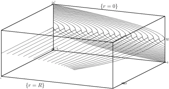
Figure 3.1: The center, stable, and unstable manifolds for twenty radial solutions to (3.13)-(3.15) with different initial values u(0) =a >0. The dotted line in the plane{r = 0} is the
u-axis (the leftmost point along this axis is the origin); this forms the center manifold for each point (a,0,0). The S-shaped curves are the stable manifolds in{r= 0}, and each curve moving into r >0 space is an unstable manifold for one of the initial conditions (a,0,0).
this is the well-understood case.) Hence each (a,0,0) has a 1-dimensional stable manifold
Ws
p((a,0,0)), a 1-dimensional unstable manifold Wpu((a,0,0)), and a 1-dimensional center manifold Wpc((a,0,0)).
An eigenvector for the eigenvalue 0 is parallel to the u-axis; by invariant manifold theory, the u-axis is the (global) center manifold Wc
p((a,0,0)) for each a ∈ R. The global stable manifold to (a,0,0) is the vertical line `a = {(a, ω,0) : ω ∈ R} in the case p = 2; for 1< p <2, the stable manifold is tangent to the vertical vector (0,1,0) at (a,0,0). We note that the S-shape of the stable manifold in the plane{r = 0}when p6= is due to the presence of |ω|2p−−p1 in (3.13)-(3.15). See Figure 3.1 for a picture illustrating these manifolds at several values of a >0.
Henceaplays the role of a parameter, and we are interested in examining howWpu((a,0,0)) behaves for different values of a. We define
Wpu,c = [ a>0
this union forms a two-dimensional “center-unstable” manifold whose winding behavior we will track in Section 3.4 until it intersects the plane {r=R}. This intersection is nonempty: as t grows large in (3.13)-(3.15), r=et will grow large as well. In fact,Wu,c
p must contain the point (0,0, R)∈Wu
p((0,0,0)). Any point lying on Wu,c
p is part of a solution that tends to (a,0,0), a >0, as t→ −∞. These solution trajectories, determined by the choice of a, foliateWpu,c. Thus we can denote any such solution by
(u(t, a), ω(t, a), r(t)).
To be more concise, we will occasionally write the above solution as
(u(t), ω(t), r(t))a
to mean (u(t), ω(t), r(t))a→(a,0,0) as t→ −∞. 3.1.2 Dynamical system in (y, w, r)-coordinates
We will make use of an Emden–Fowler transformation to exert extra control over the equations. Let λ∈R; the Emden–Fowler transformation for (3.8) is
y=rλu, (3.18)
Substituting (3.18) into (3.8) yields
0 = (p−1)rλ(1−p)
y0− λ
ry p−2
λ(λ+ 1)
r2 y−
2λ r y
0
+y00
(3.19)
+n−1
r r
λ(1−p)
y0− λ
ry p−2
y0− λ
ry
+f(r−λy).
Set z =y0− λ
ry so that
z0 =y00+ λ
r2y− λ ry
0
. (3.20)
Then the differential equation (3.19) becomes
(p−1)rλ(1−p)|z|p−2
z0− λ
rz
+ n−1
r r
λ(1−p)|z|p−2
z+f(r−λy) = 0. (3.21)
We define w byrz =w|w|2p−−p1 to obtain the following relations:
z0 = −1
r2w|w|
2−p p−1 + 1
r
1
p−1|w| 2−p
p−1w0, (3.22)
|z|p−2z = r1−pw, (3.23)
|z|p−2
z0−λ
rz
= −r−pw(1 +λ) + 1
p−1r
1−pw0
. (3.24)
Substituting (3.22)-(3.24) into (3.21) yields
(p−1)rλ(1−p)
−r−pw(1 +λ) + 1
p−1r
1−pw0
+ (n−1)rλ(1−p)r−pw+f(r−λy) = 0, (3.25)
which can be solved for w0:
w0 = ((p−1)λ−n+p)1
rw−r
p+pλ−λ−1
f(r−λy). (3.26)
To relate w to the original variable u, we note here that wcan be written in terms of u as
w=u0|u0|p−2
We note that w allows us to write (3.19) as a system of first-order equations. Defining w
by (3.27) at the same step as (3.18) allows one to bypass the calculations in (3.19)-(3.25) to obtain the first-order system immediately. We remark that (3.27) does not reduce to the samew in the Emden–Fowler coordinate system in the proof by Clemons and Jones of the case p= 2. In particular, in [7] the first equation is y0 =w/r, whereas we have the following system:
y0 = λ
ry+
1
rw|w|
2−p
p−1, (3.28)
w0 = ((p−1)λ−n+p)1
rw−r
(p−1)(1+λ)f(r−λy) (3.29)
r0 = 1, (3.30)
where 0 = ∂r∂. As in the u-coordinate system, we rescale by parametrizing r asr =et; notice
t and r have the same meaning before and after the Emden–Fowler transformation. The resulting equations are
˙
y = λy+w|w|2p−−p1, (3.31)
˙
w = ((p−1)λ−n+p)w−rp+λ(p−1)f(r−λy) (3.32) ˙
r = r, (3.33)
where·= ∂t∂. As before, the limitr→0 is equivalent tot→ −∞; for the limit of (3.31)-(3.33) to exist as t → −∞, we need to ensure that the quantity rp+λ(p−1)f(r−λy) exists in the limit. Let us treat y as independent of λ and set u = r−λy. Then if λ > 0 and y → 0 such that
u=r−λy→u
0 >0, where u0 is finite, then
lim r→0r
p+λ(p−1)
f(r−λy)
exists if λ≥ −p/(p−1). This condition happens automatically if λ≥0.
y0 <∞, then u=r−λy→ ∞. Using (R), we can compare f to rp−λ(q1−p)yq1−1 and obtain
lim r→0
rp+λ(p−1)f(r−λy)
rp−λ(q1−p)yq1−1 = limr→0
rp+λ(p−1)f(r−λy)
rp+λ(p−1)(r−λy)q1−1 =`.
Thus if the limit of rp−λ(q1−p)yq1−1 is finite as r→0, then limit of rp+λ(p−1)f(r−λy) is finite as well. We therefore require
λ≤ p
q1−p =: ˆλ, (3.34)
and we treat this number as an upper bound for λ. We will not requireλ to be nonnegative, however, and we make a note of the effect that setting λ < 0 has on the dynamics of (3.31)-(3.33) in Section 3.2.
In the ( ˙u,ω,˙ r˙) system, each point (a,0,0) is a fixed point. The analog under the Emden– Fowler transformation is the origin; linearization of (3.31)-(3.33) at the origin yields
λ 0 0
0 (p−1)λ−n+p 0
0 0 1
if p6= 2,
λ 1 0
0 λ−n+ 2 0
0 0 1
if p= 2, (3.35)
with eigenvalues{λ,(p−1)λ−n+p,1}. Notice that ifp∈(1,2), the eigenvectors are parallel to the axes; see Figure 3.1.
3.2 Critical exponents and existence of solutions
Studying uniqueness amounts to understanding how the manifold Wpu,c evolves as the radius r increases to some chosen value R; in particular we study how many times Wu,c
3.2.1 Wu,c
p under the Emden–Fowler transformation
Let T[·] be the Emden–Fowler transformation (3.18) from (u, ω, r) to (y, w, r), and let
T Wu,c p
=Wfp. Whenever r > 0 and the Emden–Fowler parameter λ satisfies 0 < λ ≤λˆ, then any point T [(u(t), v(t), r(t))a] on Wfp now satisfies
(y(t), w(t), r(t))→(0,0,0) as t→ −∞.
Thus choosingλ ∈(0,λˆ] has the effect of “blowing down” theu-axis. As a consequence, it no longer makes sense to parametrize solutions via their limit as t→ −∞. To employ a similar notion, the notation y(t, a) and (y(t), w(t), r(t))a will mean that the solution (u(t), ω(t), r(t)) obtained from y=rλu satisfies (u(t), ω(t), r(t))→(a,0,0) as t → −∞.
Assuming the critical exponent inequalities (3.2) are satisfied and p∈(1,2), we describe below the behavior of the invariant manifold Wfp.
Invariant manifold structure if λ > ˆλ. We will never consider this case as we require
λ ≤ λˆ. As it may be interesting in future problems, we note here that should one choose
λ > λˆ, then the limit of ( ˙y,w,˙ r˙) as t → −∞ is undefined. However, the manifold Wpu,c
derives from the (u, ω, r)-system and therefore exists independently of λ. For any ε > 0,
T[Wu,c
p ∩ {ε≤r ≤R}] is a two-dimensional manifold with boundary. Selecting λ >λˆ and defining Wfp as
f
Wp =T[Wpu,c∩ {ε≤r ≤R}] (3.36)
yields a well-defined two-dimensional manifold with boundary in (y, w, r)-space.
two-dimensional unstable manifold of the origin.
Invariant manifold structure if λ = 0. Ifλ = 0, then the Emden–Fowler transformation is simply u=y. HenceWfp is identical to Wpu,c, a two-dimensional center-unstable manifold.
Invariant manifold structure if λ <0. If λ <0, then there is one positive eigenvalue of (3.35) and two negative eigenvalues,
{λ,(p−1)λ−n+p}.
Thus all trajectories on the plane {r = 0} tend to the origin as t → ∞. If λ 6= np−2−p, these eigenvalues are distinct. In this case, fWp transforms to a two-dimensional stable-unstable manifold composed of the unstable manifold of the origin and the 1-dimensional subspace of the origin in {r = 0} associated with the eigenvalue λ; this is the subspace tangent to the
y-axis at the origin.
As in Section 3.2.1, if we select λ <0, then we define Wfp by (3.36) for an appropriately small ε >0.
3.2.2 Existence of solutions
In this section, we list two expressions for each ˙wequation: the first leavesf in its general form (where we assume f is odd), while the second uses (3.6). Recall equations (3.31)-(3.33):
˙
y = λy+w|w|2p−−p1 ˙
w = ((p−1)λ−n+p)w−rp+λ(p−1)f(r−λy) = ((p−1)λ−n+p)w−rp+λ(p−q1)|y|q1−2
y+νrp+λ(p−q2)|y|q2−2 y,
˙
At this point, we have not specified any particular λ; the choice we make to demonstrate the existence of solutions is λ = ˆλ. This selection characterizes Wfp as described above in Section 3.2.1, and moreover, this choice is ideal as (3.31)-(3.33) simplifies to
˙
y = ˆλy+w|w|2p−−p1 ˙
w = ((p−1)ˆλ−n+p)w−rp+ˆλ(p−1)f(r−λˆy) = ((p−1)ˆλ−n+p)w− |y|q1−2y+νrp−p(p−q2)
p−q1 |y|q2−2y,
˙
r = r,
which in the invariant plane {r= 0}reduces to
˙
y = ˆλy+w|w|2p−−p1 (3.37)
˙
w = ((p−1)ˆλ−n+p)w−rp+ˆλ(p−1)f(r−λˆy)
r=0
(3.38) = (pλˆ−n+p)w−λwˆ − |y|q1−2y. (3.39)
If it were the case that pˆλ−n+p= 0, then this system would be Hamiltonian in the plane {r= 0} with
H(y, w) = ˆλyw+ p−1
p |w|
p p−1 +
Z
rp+ˆλ(p−1)f(r−ˆλy)
r=0
dy (3.40)
= ˆλyw+ p−1
p |w|
p p−1 + 1
q1
|y|q1.
However, whenever λ= ˆλ,
pλˆ−n+p > −p 2
p−q1
+ pq1
p−q1
+p= 0. (3.41)
y ω
Figure 3.2: The stable and unstable manifolds of (y, w, r) = (0,0,0) in the {r = 0} plane, with p= 1.5, d= 3, and q1 = 2.5. The manifold spiraling outward is the unstable manifold.
inside of the curve H(y, w) = 0 while the unstable manifold appears to spiral outwards. It is a result of Franca [17] that this occurs for a large class of nonlinearities.
We can now explore precisely why we require (3.2) to be satisfied. The different dynamics corresponding to different values ofq1, with (n, p) = (3,1.8), in the{r= 0}-plane are pictured
Figure 3.3. Notice the switching of roles between the stable and unstable manifolds of (0,0,0) as q1 is varied to be below, in and above the inequalities in (3.2).
As Theorem 3.0.2 is concerned with uniqueness, rather than existence, we will not explore existence further in this chapter.
3.3 Variational equations 3.3.1 Definitions
For any time τ ∈R, we define the intersection curve
Figure 3.3: Varying q1 with (n, p) = (3,1.8) to show the stable and unstable manifolds of
(y, w, r) = (0,0,0) in the {r = 0} plane. (a) is less than the lower bound, (b) is the lower bound, (c) is within the bounds, (d) is at the Sobolev critical exponentp∗, and (e) is above
For any chosen u with initial conditionα >0, let C(τ, α) be the truncated intersection curve
defined by
C(τ, α) ={(u(τ), ω(τ), r(τ))a∈C(τ) : a∈(0, α]}.
Notice C(τ, α)⊂C(τ) lie in the{r =r(τ)}-plane. The curve defined by
γ(τ, α) ={(u(t), ω(t), r(t))α : t∈(−∞, τ]},
which we will refer to as a solution trajectory, limits to (α,0,0) as t→ −∞ and intersects
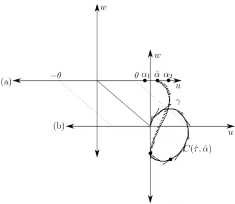
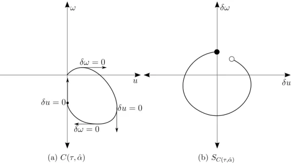
C(τ, α) at u(τ, α). Examples of both of these curves are sketched in Figure 3.4. 3.3.2 Variational equations
For any choice of t∈R, the curve C(t) in (3.42) can be parametrized by theu-coordinate initial condition a via
ct(a) = (u(t, a), ω(t, a), r(t)). (3.43)
Taking the derivative along ct(a) with respect to a yields a family of tangent vectors with
δr ≡0:
dct
da(α) =
∂u(t, a)
∂a
a=α
, ∂ω(t, a) ∂a
a=α
, ∂r(t) ∂a
a=α
=: (δu(t, α), δω(t, α),0). (3.44)
Notice that in the{r= 0}-plane, we can parametrize the center manifold in the same fashion as c{r=0}(a) = (a,0,0), and thus
dc{r=0}
da (α) = (1,0,0).
Hence
lim
The variational equations to describe how such a family of tangent vectors in the (u, ω, r )-system is carried under the flow are given by
˙
δu = 1
p−1|ω| 2−p
p−1 δω, (3.45)
˙
δω = (p−n)δω− ∂
∂u(r
pf(u)) δu− ∂
∂r(r
pf(u)) δr (3.46) ˙
δr = δr. (3.47)
In particular, the tangent vector field in (3.44) satisfies
˙
δu = 1
p−1|ω| 2−p
p−1 δω, (3.48)
˙
δω = (p−n)δω−rpf0(u)δu (3.49) ˙
δr = 0. (3.50)
We define two curves in the tangent bundle toWu,c
p as follows: for any point (u(τ), ω(τ), r(τ))a∈
C(τ, α), we find the tangent vector from (3.44) and form the following curve:
SC(τ,α)={δu(τ, a), δω(τ, a),0) : a ∈(0, α]}.
Similarly, for each point (u(t), ω(t), r(t))α along a single solution trajectoryγ(τ, α), we find the tangent vector
(δu(t, α), δω(t, α),0)
defined by (3.44) and then construct the following curve:
Sγ(τ,α) ={(δu(t, α), δω(t, α),0) : t∈(−∞, τ]}.
Figure 3.4 illustrates the tangent vectors that define these curves.
u
u w
w
(a)
(b)
α1 α αˆ 2
−θ θ
C(ˆτ ,αˆ)
γ
curve cτ(a) : [0, α]→R2. To state the definition ofI, we first define a continuous angle mea-sureϑ :cτ(a)→R so thatϑ(cτ(a)) is on the appropriate branch of arctan(δω(τ, a)/δu(τ, a)), where (δu(τ, a), δω(τ, a)) is the tangent vector along cτ(a) at the point (u(τ, a), ω(τ, a)). Moreover,
ϑ(cτ(0))≡arctan
δω(τ,0)
δu(τ,0)
∈−π 2,
π
2
. (3.51)
We remark that for 1< p <2, the angle ϑ(cτ(0)) is strictly between −π/2 and π/2, as along the invariant line {(0,0, r) | r ≥ 0}, the first component δu has ˙δu ≡ 0 by (3.45). Hence
δu≡1 along {(0,0, r)|r≥0}, and therefore (3.51) is defined for every τ. (The case p= 2 is done in [21].)
The winding number I along the intersection curve is defined by
I(cτ(a)) =
1 2
−2ϑ(cτ(α))
π + 1
− 1 2
−2ϑ(cτ(0))
π + 1
= 1 2
−2ϑ(cτ(α))
π + 1
;
the symbol b·c denotes the greatest integer function. To show that it does indeed reduce to the right-hand side and demonstrate how this calculation works, notice
ϑ(cτ(0)) ∈ −π 2, π 2
−2ϑ(cτ(0)) ∈ (−π, π) −2ϑ(cτ(0))
π ∈ (−1,1)
−2ϑ(cτ(0))
π + 1 ∈ (0,2)
1 2
−2
ϑ(cτ(0))
π + 1
∈ (0,1)
1 2
−2ϑ(cτ(0))
π + 1
= 0.
(a) δu δω a2 a3 a4 a5 a6 a7 a8 a9 a10 (b)
Point ϑ(cτ(a)) I(cτ(a))
a= 0 π/3 0
a=a2 0 0
a=a3 −π/2 1
a=a4 −5π/4 1
a=a5 −3π/2 2
a=a6 −5π/3 2
a=a7 −5π/2 3
a=a8 −11π/4 3
a=a9 −5π/2 3
a=a10 −7π/3 2
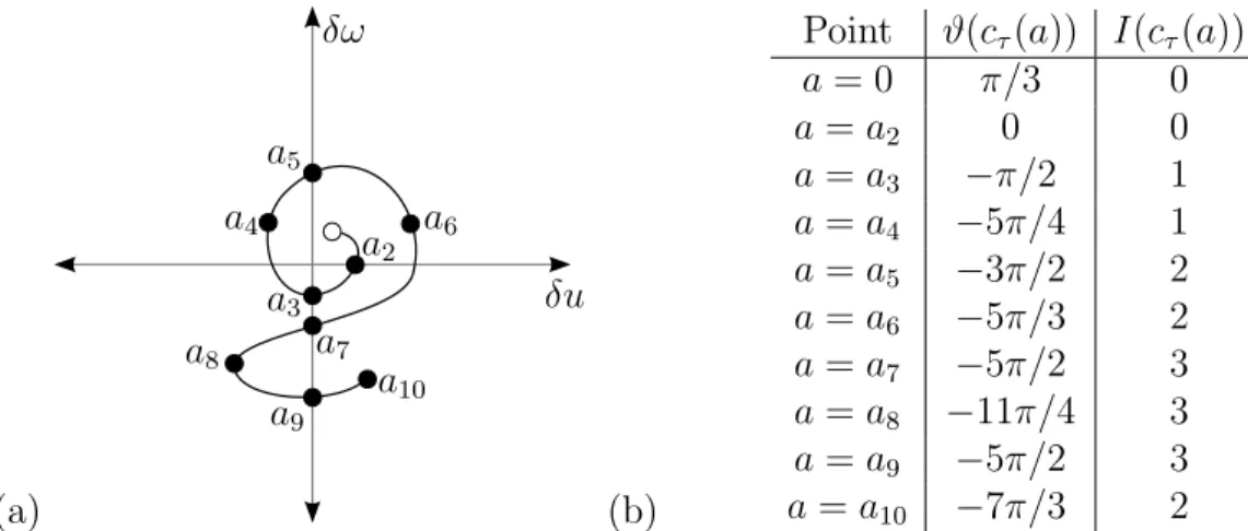
Figure 3.5: (a) An imagined SC(τ,αˆ) with 10 selected points. In (b), we estimate the angle
measure ϑ for each of the 10 points, beginning with the open circle and moving in the direction of increasing initial condition a. For each ϑ, we compute the winding numberI in the third column.
plane. See Figure 3.5 for a demonstration; this demonstration is particularly important as it shows how the winding number is calculated when the curve SC(τ,a)
a≤α stops on the δω-axis. We establish a convention in this chapter that in winding number drawings, we mark the beginning of the curve,cτ(0), with an open circle.
We use the word “homotopic” for curves to refer to the notion of being pathwise homotopic into the punctured plane R2\{0}. The winding number I is then invariant for homotopic
curves. Let us consider the piecewise-defined curves {(0,0, r)|0≤r ≤r(τ)} ∪C(τ, α) and {(a,0,0)|0≤a≤α} ∪γ(τ, α). As they form the boundary of the region
{0≤r≤r(τ)}\ (
[
0<a<α
Wpu((a,0,0)) )
,
there is a piecewise smooth path homotopy between these two curves. Thus the winding number along them must be the same. However, δu ≡ 1 along both pieces {(a,0,0) |0 ≤
a≤α} and {(0,0, r)|0≤r≤r(τ)}. Thus any winding behavior happens along C(τ, α) and
γ(τ, α). Hence we conclude thatI(SC(τ,α)) =I(Sγ(τ,α)).
δu δω
Sγ
direction of δu
direction of δu
direction of δu direction of δu
Figure 3.6: An imagined Sγ(τ,α) from Lemma 3.3.1 satisfying ˙δu = p−11 |ω|
2−p
p−1. The open circle on theδu-axis indicates that the limit ast → −∞ofSγ(τ,α) is (1,0). The closed circle on the δω-axis indicates that at the moment this winding number is computed for this particular trajectory, δu(τ, α) = 0 with δω(τ, α)>0. The winding number of the curve Sγ(τ,α) in this
case is 4.
Proposition 3.5 from [21].
Lemma 3.3.1. For any trajectory (u(t), ω(t), r(t))α at time t = τ, I(Sγ(τ,α)) is the exact
number of zeros of δu(t, α) for −∞< t≤τ.
This is not immediate: in a winding number calculation, it is possible for crossings (instances where δu= 0) to cancel each other out if they cross with δω >0 or δω <0 in the opposite direction. We see, therefore, that I(Sγ(τ,α)) is at the very least a lower bound on the
number of times δu= 0. To prove this lemma, therefore, we must show that along γ(τ, α), the winding curve can only cross the axis {δu = 0} in one direction, namely in a manner clockwise about the origin.
Proof. This lemma relies on the fact that ˙δu= p−11 |ω|2p−−p1 δω. Consider the (δu, δω)-plane as pictured in Figure 3.6. We notice immediately thatSγ(τ,α) can never intersect the origin, as δu=δω = 0 is invariant in (3.48)-(3.48), and the limit of (δu, δω) as t→ −∞ is (1,0). The fact that whenever r >0, the relation
δω = 0 ⇐⇒ δu˙ = 0 (3.52)
implies that any time Sγ(τ,α) crosses theδu-axis (i.e., the line{δω = 0}), then ˙δu= 0. Hence
the Sγ(τ,α) must be perpendicular to theδu-axis at any such crossing. Conversely, the curve
can only turn vertical if it is crossing the δu-axis. Thus there are no tangential intersections of either axes.
Furthermore, as the sign of δω and ˙δu must be the same, then δu must be increasing in the first and second quadrants, and decreasing in the third and fourth quadrants. Thus if it crosses the δω-axis with δω < 0, it must be crossing from the fourth quadrant to the third quadrant, and if it crosses the δω-axis withδω >0, it must be crossing from the second quadrant to the first quadrant. Hence each crossing of the line {δu = 0} must be in the clockwise direction. Therefore, the winding number I(Sγ(τ,α)) is equal to the exact number of
zeros of δu. A whimsical example of an Sγ(τ,α) that follows these guidelines is pictured in
Figure 3.6.
Recalling that T is the Emden–Fowler transformation, we consider the intersection curve in Emden–Fowler coordinates by computing
D(t) = T(C(t)).
parametrized by a. Define
dDt
∂a (α) =
∂y(t, a)
∂a
a=α
, ∂w(t, a) ∂a
a=α
, ∂r(t) ∂a
a=α
=: (δy(t, α), δw(t, α),0). (3.53)
Under the Emden–Fowler transformation, the variational equations for the (y, w, r)-system are given by
˙
δy = λ δy+ 1
p−1|w| 2−p
p−1 δw, (3.54)
˙
δw = ((p−1)λ−n+p)δw− ∂
∂y r
p+λ(p−1)
f(r−λy)
δy (3.55)
− ∂
∂r r
p+λ(p−1)
f(r−λy) δr
˙
δr = δr. (3.56)
Notice in particular that the vector field (δy(t), δw(t),0)α satisfies (3.54)-(3.56) with δr ≡0. As y=rλu, along this vector field we can write
δy|δr=0 = λrλ−1u δr+rλδu
δr=0 =r
λδu. (3.57)
There are therefore three cases for limt→−∞δy:
1. if λ >0, thenδy →0,
2. if λ= 0, then δy →1, and
3. if λ <0, then the limit of δy is undefined.