The single-index hazards model

(1)

THE SINGLE-INDEX HAZARDS MODEL

Kai Ding

A dissertation submitted to the faculty of the University of North Carolina at Chapel Hill in partial fulfillment of the requirements for the degree of Doctor of Philosophy in the Department of Biostatistics, Gillings School of Global Public Health.

Chapel Hill 2010

Approved by:

Dr. Michael Kosorok, Advisor

Dr. Donglin Zeng, Advisor

Dr. Amy Herring, Reader

Dr. Jason Fine, Reader

(2)

c ° 2010 Kai Ding

(3)

Abstract

KAI DING: THE SINGLE-INDEX HAZARDS MODEL.

(Under the direction of Dr. Michael Kosorok and Dr. Donglin Zeng.)

We first propose the single-index hazards model for right censored survival data. As

an extension of the Cox model, this model allows nonparametric modeling of covariate

effects in a parsimonious way via a single-index. In addition, the relative importance of

covariates can be assessed via this model. We consider the conventional profile-kernel

method based on the local likelihood for model estimation. It is shown that this method

may give consistent estimation under certain restrictive conditions, but in general it

can yield biased estimation. Simulation studies are conducted to demonstrate the bias

phenomena. The existence and nature of the failure of this commonly used approach is

somewhat surprising.

The interpretation of covariate effects in the aforementioned single-index hazards

model is difficult. Thus, we further propose the partly proportional single-index

haz-ards model in which the effect of covariates of primary interest is represented by the

regression parameter while “nuisance” covariates can have nonparametric effect on the

survival time. We again consider the conventional profile-kernel method and it leads to

biased estimation as well. A bias correction method is then proposed and the corrected

profile local likelihood estimators are shown to be consistent, asymptotically normal and

semiparametrically efficient. We evaluate the finite-sample properties of our estimators

through simulation studies and illustrate the proposed model and method with an

appli-cation to a dataset from the Multicenter AIDS Cohort Study (MACS).

Besides the profile-kernel method, we also study the profile stratified likelihood method

(4)

may give consistent estimation under the restrictive “independent censoring” condition,

but in general it can yield biased estimation. Simulation studies are conducted to

demon-strate the situations in which the bias phenomena do (or do not) exist; In the partly

proportional single-index hazards model, we demonstrate numerically the existence of

the bias and then propose a bias correction method. The estimators from the corrected

profile stratified likelihood method are shown to be consistent. Their finite-sample

prop-erties are evaluated through simulation studies. The corrected profile stratified method

is applied to the aforementioned MACS study for illustration.

(5)

Acknowledgments

This dissertation could not have been written without my advisors, Dr. Michael Kosorok

and Dr. Donglin Zeng, who led me to this research field and patiently guided me through

the dissertation process. I wish to express my deepest appreciation to them for their

support, encouragement and mentoring.

I owe many thanks to the rest of my committee members. I am deeply grateful to Dr.

Amy Herring for her insightful advice, more than 3 years of financial support and being

my academic advisor. My thanks also goes to Dr. Jason Fine and Dr. David Richardson

for their invaluable advice and kindness throughout this research.

I would also like to thank all of my friends, particularly Yi Gong, Qianchuan He,

Yijuan Hu, Zhaowei Hua, Yiyun Tang, Yingqi Zhao and Yufan Zhao, whose friendship

has made this journey more enjoyable and memorable.

Finally, it’s impossible to have completed this journey without the love, support and

(6)

List of Figures

2.1 Profile local likelihood curve of γ1 in single-index hazards model . . . 23

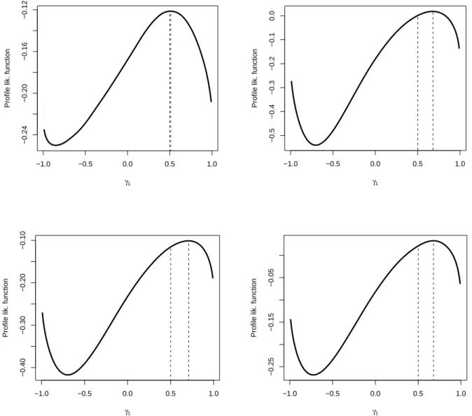
3.1 Profile local likelihood curve of γ1 in PPSIH model . . . 36

3.2 Profile local likelihood curves (corrected and uncorrected) of γ1 in PPSIH

model . . . 41

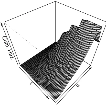
3.3 Cumulative baseline hazard estimator ˆΛ(t, u) under PPSIH model (2). . . 45

4.1 Profile stratified likelihood curve of γ1 in single-index hazards model . . . 65

4.2 Profile stratified likelihood curve of γ1 in PPSIH model . . . 70

4.3 Profile stratified likelihood curves (corrected and uncorrected) of γ1 in

PPSIH model . . . 74

(9)

List of Tables

2.1 Simulation results of local likelihood in single-index hazards model . . . . 22

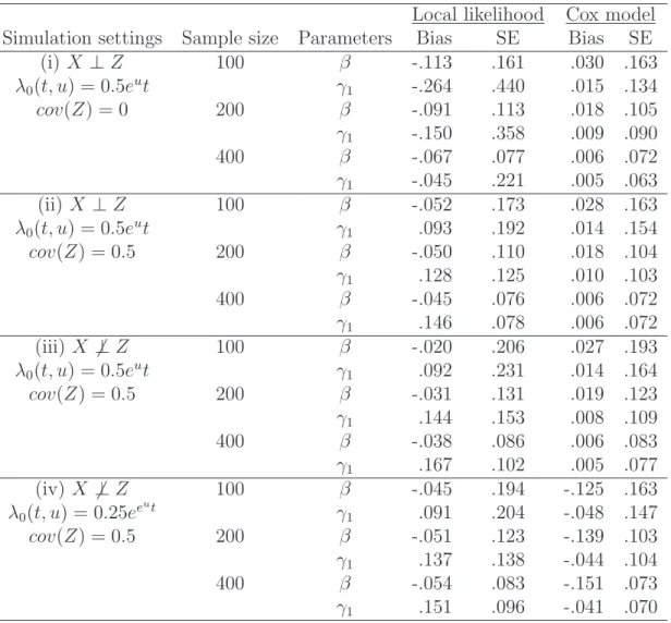
3.1 Simulation results of local likelihood in PPSIH model . . . 35

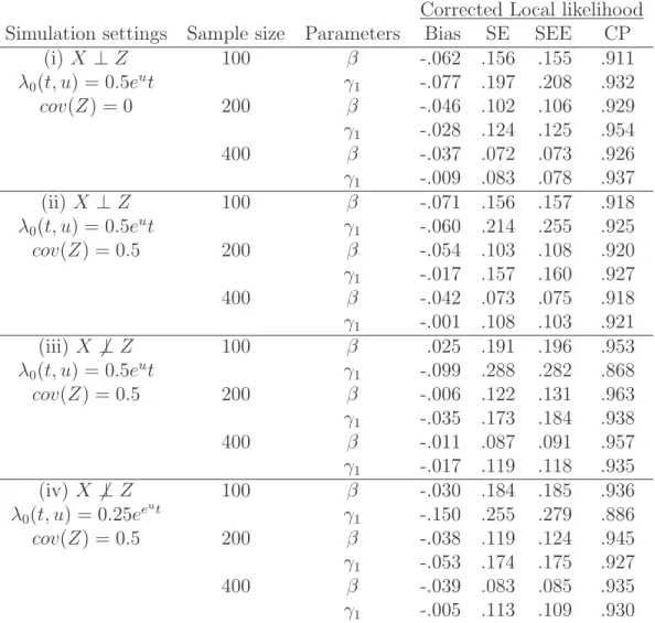
3.2 Simulation results of corrected local likelihood in PPSIH model . . . 40

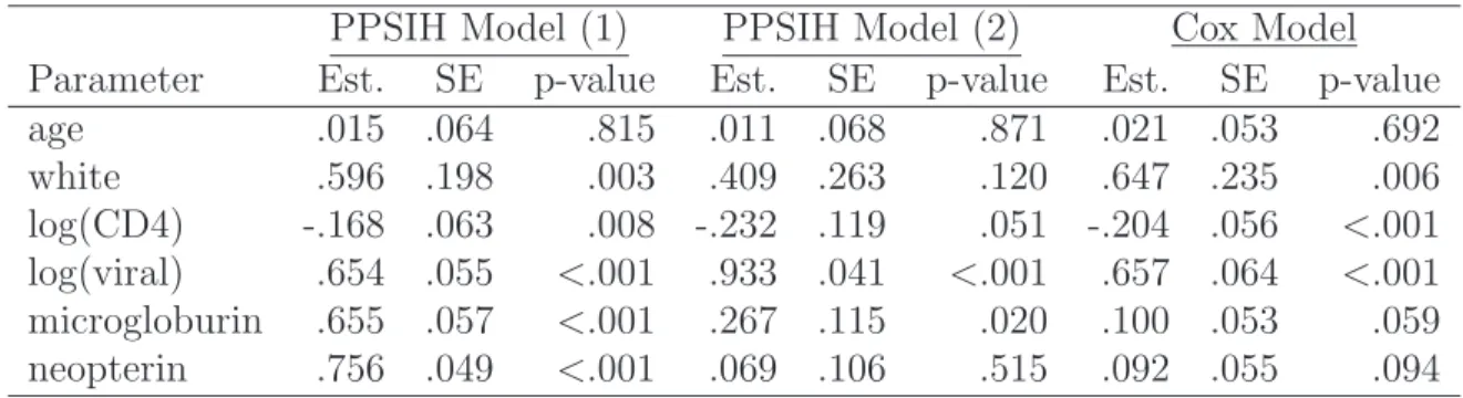
3.3 Analysis of MACS Data under PPSIH Model (1), (2) and Cox Model . . 44

4.1 Simulation results of stratified likelihood in single-index hazards model . 64

4.2 Simulation results of stratified likelihood in PPSIH model . . . 69

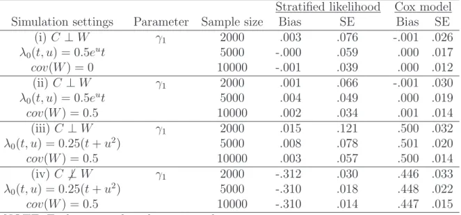
4.3 Simulation results of corrected stratified likelihood in PPSIH model . . . 73

(10)

Chapter 1 Introduction

1.1 Motivation and Literature Review

1.1.1 Semiparametric and Nonparametric Regression Models

for Survival Data

In survival analysis, investigators often wish to assess the effect of covariates on the risk of

the event of interest. For example, in the Multicenter AIDS Cohort Study (MACS), one

important research question is to evaluate the effect of patient’s baseline age, ethnicity,

CD4 positive cell counts, viral loads, serumβ2-microgloburin levels and serum neopterin

levels on survival time (i.e. time to death due to AIDS) among HIV positive men. The

four biomarkers (CD4 positive cell counts, viral loads, serum β2-microgloburin levels

and serum neopterin levels) were identified as the most predictive prognostic factors in

Mellors et al. (1997). The Cox proportional hazards model (Cox 1972) is a popular and classical choice in such scenarios due to its nice interpretation of regression parameters

and the availability of efficient inference procedures implemented in all statistical software

packages. In this model, the conditional hazard rate of failure time given covariates,

denoted by W, is modeled as h(t|W) = λ(t)eβT_W

, where λ(·) is a completely unknown

(11)

log-hazard ratios of the covariates W. Cox (1975) also proposed the partial likelihood to estimate the regression parameters. The by now classical large sample properties of

the partial likelihood estimators were later proved inAndersen and Gill (1982). See also Fleming and Harrington (1991) and Andersen, Borgan, Gill, and Keiding (1993) for the literature concerning this model.

An underlying assumption of the Cox model is the so-called proportional hazards

assumption, that is, the hazard ratio remains constant over time or covariates have

log-linear effects on the risk of the event of interest. However, in many real datasets,

covariates may exhibit much more complicated effects than log-linear effects; thus the

proportional hazards assumption may be violated and the Cox model may not be an

appropriate choice. For example, in the aforementioned MACS data, testing for the

proportional hazards assumption based on martingale residuals (Lin, Wei, and Ying 1993)reveals that the covariate viral load (after taking logarithmic transformation) does not satisfy this assumption (p=.006). Thus the inference based on the Cox model may

not be valid due to model misspecification.

For this reason, many authors have considered alternatives or extensions of the Cox

proportional hazards model. For example, the accelerated failure time model (Cox and Oakes 1984, chap. 5) is attractive due to its direct physical interpretation. This model takes the form logT =−βT_W ₊_{², where} _T _{denotes the survival time,} _² _{is independent} of W and has an unspecified distribution. Note that by assuming this model, the

covari-ates W have effects on the survival time and so the interpretation is direct. The rank

estimator was studied by Prentice (1978) and the least-squares estimator was studied by Buckley and James (1979). Neither estimator achieves the semiparametric efficiency bound defined in Bickel, Klaassen, Ritov, and Wellner (1993). Recently, Zeng and Lin (2007a)provided a computationally tractable and semiparametrically efficient estimator for the regression parameter β using a kernel approximation of the profile likelihood.

(12)

Alternatively, instead of assuming a constant hazard ratio over time as in the Cox

model, the proportional odds model (Bennett 1983; Pettitt 1984) assumes the odds ratio of survival to be constant over time. Consequently, the ratio of the hazards converges

to unity as time increases. The model takes the form −log{ST|W(t)/(1−ST|W(t))} = G(t)+βT_W_{, where}_S

T|W(·) denotes the conditional survival function ofT given covariates

W and G(t) = log{F(t)/(1−F(t))}. Here F(t) =P(T ≤t) is the baseline distribution function of the survival timeT. The maximum likelihood estimation for this model was

studied by Murphy, Rossini, and van der Vaart (1997). The profile likelihood estimator for the regression parameter was shown to be consistent, asymptotically normal and

semiparametrically efficient. They also provided the profile likelihood ratio test for the

regression coefficient β.

The Cox proportional hazards model and the proportional odds model are special

cases of the generalized odds-rate model considered in Scharfstein, Tsiatis, and Gilbert (1998). The odds-rate model takes the form gρ(ST|W(t)) = α(t) +βTW, where ST|W(t) has the same meaning as in the proportional odds model, gρ(x) equals log(ρ−1(x−ρ−1)) when ρ > 0 and equals log(−log(x)) when ρ = 0 and α(·) is some arbitrary increasing

function. If ρ = 0, this model is equivalent to the Cox proportional hazards model and

if ρ = 1, this model reduces to the proportional odds model. Scharfstein et al. (1998) showed that the nonparametric maximum likelihood estimator forβis semiparametrically

efficient.

Another general model which includes the proportional hazards model and the

pro-portional odds model as special cases is the propro-portional hazards frailty regression model

studied in Kosorok, Lee, and Fine (2004). In this model, the conditional hazard takes the formh(t|W, U) =λ(t)eβT_W_+log(_U₎

, whereU is a continuous frailty with mean 1 within

a known one-parameter family of distribution and λ(·) is an unspecified baseline hazard

function. That is, the hazard given the covariates W and a random frailty U unique

to each individual has the proportional hazards form multiplied by the frailty. A robust

(13)

nonparametric likelihood-based inference was carried out to allow for model

misspecifica-tion. The profile likelihood estimators for the finite dimensional parameters were shown

to be semiparametric efficient when the model is correctly specified. It was also proved

inKosorok et al. (2004)that the bootstrap gives valid inferences for all parameters, even under model misspecification.

An even more general class of models which includes the generalized odds-rate model

as its special case is the class of linear transformation models (Dabrowska and Doksum

1988;Slud and Vonta 2004;Zeng and Lin 2007b) with the formH(t|W) =G(Λ(t)eβT_W

),

where H(·|W) denotes the conditional baseline cumulative hazard function given

co-variates W, Λ(·) denotes the baseline cumulative hazard function and both G(·) and

Λ(·) are unspecified. Equivalently, the linear transformation model can be written as

Λ(T) =−βT_W ₊_{², where Λ(·) is an unspecified increasing function and} _² _{is a random} error with a specified parametric distribution. The choice of the extreme value and

stan-dard logistic error distributions yield the proportional hazards and proportional odds

model, respectively. In particular,Zeng and Lin (2007b)proposed a very general class of transformation models for counting processes which encompasses linear transformation

models and which accommodates time-varying covariates and recurrent events and they

also proved the semiparametric efficiency for the estimator of the regression parameter

using nonparametric maximum likelihood estimation (NPMLE).

Among other extensions of the Cox model is the fully nonparametric model of the

formh(t|W) =λ(t, W) studied byNielsen and Linton (1995), where the functionλ(·,·) is unspecified. One nice feature about this model is that the covariates do not need to satisfy

the proportional hazards assumption and it provides the most flexible way to model

covariate effects. A kernel estimator for the conditional hazard rate was proposed and its

uniform convergence and asymptotic normality were established. The rate of convergence

(14)

the form h(t|W) = λθ(t)g(W), where λθ(·) is the parametric baseline hazard function

indexed by a parameter θ and g(·) is completely unknown. Note that this multiplicative

model is a special case of Nielsen and Linton (1995). A kernel smoothed estimator for the nonparametric function g(·) was proposed and the estimator for the regression

parameter β was constructed based on a kernel smoothed profile likelihood function.

The resulting estimator forβ was shown to achieve the semiparametric efficiency bound.

Although assuming a parametric baseline hazard function may seem reasonable in certain

settings, it is more desirable to assume a nonparametric baseline hazard function instead

so that the model is more robust to misspecification. Furthermore, all covariates in this

model are required to satisfy the proportional hazards assumption. Instead of assuming

a parametric baseline hazard function,Fan, Gijbels, and King (1997) focused on another multiplicative nonparametric model of the formh(t|W) =λ(t)eφ(W)_{, where the logarithm}

of the conditional hazard rate function is assumed to be the sum of an unknown function

of covariates and an unknown function of the survival time. Note that this model is

also a special case of the model studied in Nielsen and Linton (1995). The estimation of φ(·) was based on its local approximation by a polynomial function and the estimation

for β was based on a local version of the partial likelihood. The estimator for β was

shown to be asymptotically normal but no results on semiparametric efficiency were

reported. Similar to the model studied in Nielsen et al. (1998), proportionality is an implicit requirement for all covariates. Note that all covariates in these three models

have nonparametric effects. Although this may seem flexible, the interpretation of the

covariate effects is difficult and the nonparametric estimation of the unknown function

in each of these models is feasible only if the dimension of W is low. That is, all these

three models suffer from the so-called “curse of dimensionality”.

(15)

1.1.2 Single-Index Models

One of the most convenient models for dimension reduction is the single-index model,

which is commonly used in biometrics and econometrics, discussed byH¨ardle and Stoker (1989)andH¨ardle, Hall, and Ichimura (1993). The model takes the formY =η(βT_W_)+², whereY denotes the response, the univariate smooth functionη(·) is completely unknown,

β is an unknown unit vector with one coordinate positive for identification purposes and

E(²|W) = 0 almost surely. Note that, in contrast to a nonparametric model of the

formY =η(W) +², the parsimonious single-index model is particularly attractive since

the original multi-dimensional covariate vector W has been replaced by a 1-dimensional

“single-index” (the linear combinationβT_W_{). Through dimension reduction in this way,}

the nonparametric estimation ofη(·) becomes feasible. Another attractive property about

this single-index model is that the relative importance of the components of W can be

fully characterized by the orientation vectorβsince the derivative ofE(Y|W) with respect toWi, theith component of the covariates W, is proportional to βi, theith component of

β. Thus βi characterizes how fast E(Y|W) changes with Wi. This piece of information on the relative importance of components of W is practically useful for designing future

studies. For instance, one only need to measure those important biomarkers but ignore

those non-important ones that may be expensive to measure. We note thatβ does not in

general represent the covariate effects as in a linear regression model. However, ifη(·) is a

monotone function, then β has the same role as “effect” parameters. Two popular

meth-ods for estimating the single-index model are the average derivative estimation method

proposed byH¨ardle and Stoker (1989)and the method of H¨ardle et al. (1993), who used the kernel smoothing method to construct the estimator of the unknown functionη(·) of

the single-index and the estimator of the orientation vectorβminimizes a modified mean

square error function. H¨ardle et al. (1993) also suggested an empirical rule for selecting the bandwidth.

(16)

covariate vector W. When the dimension of this covariate vector is high, one may wish

to include multiple principle components into the model so that “enough” information

is extracted from the covariates. Thus it may be attractive to consider a model of the

form Y = m(βT

1W,· · · , βkTW) +², where m(·) is an unknown k−variate function and E(²|W) = 0 almost surely. Here k ≥1 is a pre-specified integer less than the dimension of the covariates W. This model has been studied extensively in the literature. Recent

work includes Cook and Li (2002), Xia, Tong, Li, and Zhu (2002) and Yin and Cook (2002), among others.

Since it is likely that one of the dimension reduction components (or single-indices)

βT

1W,· · · , βkTW affects the response linearly and the other k−1 components affect the response nonlinearly, it is natural to consider a multiple-index model (Ichimura and Lee

1991; Horowitz 1998; Xia 2008; among others) of the form Y =G(βT

1W,· · · , βk−T 1W) +

βT

kW +², where E(²|W) = 0 almost surely and G(·) is an unknown link function.

Com-pared to the model with nonparametric modeling of all single-indices, this partly linear

model enjoys an easier interpretation and better estimation due to the further dimension

reduction in the unknown nonparametric function m(·). When the number of

single-indices k is large (although less than the dimension of W already), it may be beneficial

to consider the so-called additive-index model (Chiou and M¨uller 2004) of the form

Y = Pk_j₌₁mj(βjTW) +², where mj(·) is an unknown univariate function, j = 1,· · · , k, and again E(²|W) = 0 almost surely. Note that such a model replaces the unknown

function ofk variables inCook and Li (2002),Xia et al. (2002)andYin and Cook (2002) byk unknown univariate functions and thus offers a better estimation due to dimension

reduction. One special case of the additive-index model is the additive single-index model

studied by Naik and Tsai (2001)which takes the form Y =m1(αTW1) +m2(γTW2) +²,

where WT _{= (W}T

1 , W2T)T. This is a special case of the additive-index model of Chiou

and M¨uller (2004) by setting k = 2, βT

1 = (αT,0T)T and β2T = (0T, γT)T.

(17)

In the survival analysis context, the model with the conditional hazard function

spec-ified as h(t|W) = λ(t)eφ(βT_W₎

, where both λ(·) and φ(·) are unknown, was studied by

Wang (2004)andHuang and Liu (2006). Ifφ(x) =x, this model reduces to the Cox pro-portional hazards model. Note that this model is similar in form to the model studied by

Fan et al. (1997)except that the single-indexβT_W _{replaces the original covariates}_W _for dimension reduction. In Wang (2004), covariates are allowed to be time-dependent and potentially missing. When the missing covariates are present, a two stage approach was

proposed to account for the missingness. In the first stage, the missing time-dependent

covariates were imputed using functional data analysis methods. In the second stage,

a two-step iterative algorithm was performed to estimate the unknown function φ(·).

Asymptotic properties were derived for the estimator of the nonparametric function

when time-dependent covariates are not missing, but there are no asymptotic

proper-ties for the estimator of β presented in that paper. Later, Huang and Liu (2006) used spline smoothing techniques to approximate the unknown link function φ(·) and then

employed the maximum partial likelihood to estimate the regression parameter β. They

also established inference procedures for the function φ(·) and the index coefficient

vec-tor β, and discussed the interpretation of the regression coefficients in detail, but no

results on semiparametric efficiency were presented. Furthermore, in the aforementioned

two models, all of the covariates are incorporated into one single-index term, no matter

whether they have linear or nonlinear effects on the hazard and thus the interpretation of

covariate effects are difficult. Also, all covariates must meet the proportional hazards

re-quirement. Recently, Xia, Zhang, and Xu (2010) studied a very general regression model of the formT =G(BT_{W, ²), where}_T _{is the survival time,} _G(·,_{·) is completely unknown,} B is a parameter matrix with the column dimension less than the row dimension and ²

is independent of the covariates W. Note that this model includes the transformation

(18)

reduction method by introducing a nominal regression model to estimate the conditional

hazard function via estimation of the central subspace in the presence of censoring.

Sim-ilarly, this model treats all the covariates in the same way (via nonparametric modeling

of single-indices) and so the model interpretation is difficult.

It is worthwhile at this stage to point out that given a set of available covariates, one

should always screen out those covariates that are inappropriate for control before model

fitting, as suggested by Greenland (1989). For example, in epidemiologic studies, “it is well known that covariates influenced by the exposure or disease are inappropriate for

control, since control of such covariates may lead to considerable bias” (Greenland 1989);

thus, we assume throughout this dissertation that the covariates W are those remaining

after the screening. We also note that “covariates” used in this dissertation could be

other types of relevant quantities. For example, principle components are widely used

in genetics as “covariates”, as in Kong, Pu, and Park (2006), Chen, Wang, Smith, and Zhang (2008)andMa and Kosorok (2009). In the sequel, we will use “covariates” despite the note we just made.

1.1.3 Partially Linear Models for Survival Data

In all of the aforementioned models, all components ofW are treated equally in the sense

that no distinction is made as to which components are more interesting to investigators

than the others. In practice, covariatesW can often be partitioned into two parts, sayX

and Z, corresponding to the covariates of primary interest and the “nuisance” covariates

(potential confounders), respectively. We assume in the sequel that X is p dimensional

and Z is q dimensional. For example, in the aforementioned MACS data, one might be

interested in assessing the effect of patient’s ethnicity, baseline age, viral loads and CD4

counts on the risk of death due to AIDS, controlling for serum β2-microgloburin levels

and serum neopterin levels. Thus patient’s ethnicity, baseline age, viral loads and CD4

counts are treated as covariates of primary interestX and serumβ2-microgloburin levels

(19)

and serum neopterin levels are treated as “nuisance” covariates Z. One might also wish

to assess in particular the effect of patient’s ethnicity and baseline age on the risk of

death due to AIDS, controlling for the remaining 4 biomarkers. Thus in this instance the

covariates of primary interest are patient’s ethnicity and baseline age and the remaining

4 biomarkers are “nuisance” covariates.

Since covariates of primary interest are given more priority, X is often modeled

para-metrically to ensure model interpretability but Z is modeled nonparametrically to

al-low for model flexibility. One example of such a modeling strategy is the partially

lin-ear Cox model studied by Sasieni (1992a, b). The model takes the form h(t|X, Z) = λ(t)eβT_X₊_φ₍_Z₎

, where bothλ(·) andφ(·) are completely unknown. Note that by assuming

proportionality ofX through a parametric functionβT_{X, the regression parameter}_β _can

now be interpreted as the log-hazard ratio for X and the “nuisance” covariates Z can

have nonparametric effects on the hazard function. The estimation method for this model

in Sasieni (1992a, b) was based on a spline smoothed partial likelihood. Sasieni (1992a, b) also provided the efficient score and information bound for estimating β. However, no details were provided on the asymptotic distribution of the suggested spline based

estimators.

The special case when Z is 1-dimensional and λ(·) is a parametric function indexed

by a finite dimensional parameter θ in the partially linear Cox model was studied by

Lu, Singh, and Desmond (2001), who proposed to estimate β by maximizing a profile likelihood after profiling out φ(·) estimated by using the local likelihood. The resulting

estimator for (β, θ) was √n−consistent, asymptotically normal and semiparametrically efficient. Heller (2001) considered the same model as inLu et al. (2001)except assuming a nonparametric baseline hazard function. Similarly, his estimator for β was based on

a profile likelihood after profiling out the infinite dimensional parameters using kernel

smoothing. The resulting estimator for β was again shown to be semiparametrically

(20)

linear Cox model with multi-dimensional “nuisance” covariates have not been studied.

Although the partially linear Cox model is flexible in term of modeling “nuisance”

covari-ate effects, it has two potential drawbacks. First, as in Nielsen and Linton (1995), Fan et al. (1997) and Nielsen et al. (1998), the nonparametric estimation is only practically feasible when the dimension of the “nuisance” covariates Z is low; Second, “nuisance”

covariates are required to satisfy the stringent proportional hazards assumption.

To tackle the first drawback of the partially linear Cox model in Sasieni (1992a, b), Huang (1999) studied the partly linear additive Cox model by assuming h(t|X, Z) = λ(t)eβT_X₊Pq

i=1φi(Zi), where λ(·) and φ

i(·) are unknown functions and Zi is the ith

com-ponent of the q-dimensional covariates Z, i = 1,· · · , q. Thus one unknown function of q variables in Sasieni (1992a, b) has been replaced by q unknown univariate functions and so it breaks the “curse of dimensionality”. Note that this model is a special case of

Sasieni (1992a, b). The polynomial spline method was used to estimate the nonparamet-ric functions φi(·), i= 1,· · · , qand the estimators of the regression parameters maximize the induced spline smoothed partial likelihood, which were shown to be √n-consistent, asymptotically normal and semiparametrically efficient. Note that such a model requires

estimating q unknown functions and so is computationally intense. Moreover, the

“nui-sance” covariates are still required to satisfy the proportional hazards assumption.

The second drawback of Sasieni’s (1992a, b) model can be overcome by assum-ing a partly proportional hazards model (Dabrowska 1997) of the form h(t|X, Z) = λ(t, Z)eβT_X

, where λ(·,·) is an unknown bivariate baseline hazard function which de-pends on the “nuisance” covariates Z. Note that this model includes Sasieni (1992a, b) model as a special case. The parameter estimation in Dabrowska (1997) was based on a kernel smoothed partial likelihood. It was shown that when the dimension of Z is at

most 3, the estimator for β is asymptotically normal at rate √n. However, the proposed estimator fails to be√n−consistent when the dimension ofZ is larger than 3. A one-step estimator was then suggested to achieve the √n rate. Therefore, as in Sasieni (1992a,

(21)

b), this model is only practically feasible whenZ is low dimensional. Furthermore, there are no results on semiparametric efficiency in this instance.

In the current setting of semiparametric modeling of covariates effects, the

aforemen-tioned strategy for dimension reduction via a single-index can also be used. For example,

Xia, Tong, and Li (1999) studied the partially linear single-index model of the form Y =βT_X₊_η(γT_{Z) +}_{², where} _{η(·) and} _² _{are defined in the aforementioned single-index}

model. Again, the kernel smoothing method was used to construct the estimator of the

unknown function η(·) of the single-index. More generally, Carroll, Fan, Gijbels, and Wand (1997) proposed the generalized partially linear single-index model of the form g(E(Y|X, Z)) = βT_X ₊_η(γT_{Z), where} _{g(·) is a known link function and} _{η(·) is} un-specified. A local quasi-likelihood was used to estimate the unknown function of the

single-index. However, a √n−consistent pilot estimator for γ and under-smoothing are needed. Later, Xia and H¨ardle (2006) proposed the minimum average variance estima-tion method which does not require a√n−consistent pilot estimator and the bandwidth can be selected at the optimal smoothing rate. Besides kernel smoothing methods, other

smoothing methods have been studied. For example, Yu and Ruppert (2002) considered the penalized spline method in the partially linear single-index model (Xia et al. 1999)

and showed that the penalized spline method performs better than the kernel smoothing

method of Carroll et al. (1997).

In the survival analysis context, Lu, Chen, Song, and Singh (2006)considered the par-tially linear single-index survival model of the form h(t|X, Z) =λθ(t)eβT_X₊_η₍_γT_Z₎

, where

the form of the baseline hazard function is known up to an Euclidean parameter θ and

η(·) is unknown. The estimation of η(·) was based on a local linear fit and the

estima-tor for (β, γ, θ) was shown to be asymptotically normal and semiparametrically efficient.

Even though the parametric baseline hazard appears reasonable in many applications,

it is desirable to have a more flexible nonparametric hazard instead. In that direction,

(22)

model of the form h(t|X, Z) = λ(t)eβT_X₊_η₍_γT_Z₎

, where λ(·) is now unspecified. Sun et al. (2008)adopted a polynomial spline smoothing technique for estimating the unknown smooth function η(·). However, no asymptotic results were presented in this instance.

Furthermore, all covariates in Lu et al. (2006) and Sun et al. (2008) must satisfy the proportional hazards assumption.

1.2 Outline of Dissertation

In this dissertation, we first consider the “single-index hazards model”, a modification of

the model studied in Nielsen and Linton (1995), by assuming a nonparametric baseline hazard function that depends onW through a single indexβT_W_{. Specifically, we consider}

a model of the formh(t|W) = λ(t, βT_W_{), where}_λ(·,_{·) is an unknown bivariate function.} Note that this model includes the Cox model and all the transformation models mentioned

before as special cases. In addition, the model has several nice features. First, covariates

are allowed to have nonparametric effects on the hazard function. This is particularly

useful if covariates W do not satisfy the proportional hazards assumption so that the

Cox model may not be appropriate. Second, the relative importance of the components

ofW can be fully characterized by the orientation vectorβ since the derivative ofh(t|W)

with respect to Wi, the ith component of the covariate vector W, is proportional to βi,

thusβi characterizes how fast h(t|W) changes with Wi. Third, this single-index hazards

model is more parsimonious than the model inNielsen and Linton (1995)since the multi-dimensional vector W has been replaced by a one-dimensional single-index βT_W_{. The}

local likelihood approach is commonly used for the single-index model. Thus we adapt

this approach for parameter estimation in our single-index hazards model. Surprisingly,

we find, both theoretically and numerically, that this commonly used approach in general

yields inconsistent estimators and it may work only under very specific conditions.

(23)

Since the aforementioned single-index hazards model cannot in general address

co-variate effects, especially the effect of coco-variates of main interest, we further propose the

“partly proportional single-index hazards model” by assumingh(t|X, Z) =λ(t, γT_Z)eβT_X

,

where λ(·,·) is an unknown function. The model has several nice features. First, by as-suming proportionality of X via the linear combination βT_{X, the regression parameter}

β can be interpreted as the log-hazard ratio of the covariates of primary interest X

for any given Z, while Z is allowed to have nonparametric effects. The nonparametric

modeling of Z is particularly useful if the “nuisance” covariates do not satisfy the

pro-portional hazards assumption so that the Cox model may yield biased results. Second,

this model overcomes both drawbacks associated withSasieni’s (1992a, b)model. Specif-ically, it is parsimonious since the q-dimensional covariates Z have been replaced by a

one-dimensional single-index γT_{Z, and thus nonparametric estimation becomes feasible.}

Furthermore, as in Dabrowska’s (1997) model, the proportional hazards assumption is relaxed for Z. Third, similar to the single-index hazards model, the relative importance

of the components of Z can be fully characterized by the orientation vector γ since the

derivative of h(t|X, Z) with respect to Zi, the ith component of the “nuisance”

covari-ates Z, is proportional to γi, the ith component of γ. Thus γi characterizes how fast

h(t|X, Z) changes with Zi,i= 1,· · · , q. To estimate the regression parametersβ and γ, we construct a profile likelihood after profiling out the baseline hazard function, which is

estimated based on a local likelihood function. Similar to the single-index hazards model,

it is shown that this conventional profile-kernel method leads to biased estimation of the

regression parameters. We also believe that this bias phenomenon extends to other model

settings besides our partly proportional single-index hazards model. To address the bias

issue in this model, we propose a bias correction method which is shown to have nice

asymptotic properties and works well in finite-sample settings.

In addition to the profile local likelihood method, we consider another popular

(24)

stratification on the single-index. In the single-index hazards model, this method may

give consistent estimation under the restrictive “independence censoring” condition, but

in general it can yield biased estimation. Simulation studies are conducted to

demon-strate the situations in which the bias phenomena do (or do not) exist; In the partly

proportional single-index hazards model, we demonstrate numerically the existence of

the bias and then propose a bias correction method using a similar idea for correcting

the bias in the profile local likelihood method. The estimators from the corrected profile

stratified likelihood method are shown to be consistent. Their finite-sample properties

are evaluated through simulation studies and this bias corrected method is applied to

the aforementioned MACS study for illustration.

The remainder of this dissertation is organized as follows. Chapter 2 focuses on the bias analysis of the profile local likelihood approach in the single-index hazards model.

In Section 2.1, we describe the single-index hazards model and the data structure. In Section2.2, we describe how to adapt the commonly used profile local likelihood method for parameter estimation. We then study the asymptotic bias of this approach in Section

2.3 and identify conditions under which this approach may work. In Section 2.4, we demonstrate our findings via a series of simulation studies. In Chapter3, we focus on the partly proportional single-index hazards model. In Section 3.1, we describe the model and the data structure. In Section 3.2, we consider again the commonly used profile local likelihood method and study the estimation bias associated with this method, both

theoretically and numerically. A bias correction method is then proposed and results

on the asymptotic and finite-sample properties of the corrected profile local likelihood

estimator are given in Section 3.3. In Section 3.4, we illustrate the proposed model and method with an application to a dataset from the MACS. Chapter 4 studies the profile stratified likelihood method. In Section 4.1, we consider this method in the single-index hazards model and its performance is studied both asymptotically and numerically. In

Section 4.2, we consider this method in the partly proportional single-index hazards

(25)

model. Specifically, we demonstrate the estimation bias numerically, propose a bias

correction, give some asymptotic results of the corrected stratified likelihood method

and apply the partly proportional single-index hazards model to the dataset from the

MACS using the bias corrected method. Finally, the dissertation is concluded with a

(26)

Chapter 2 Single-Index Hazards Model

2.1 Model and Data Structure

We assume the following single-index hazards model

h(t|W) =λ(t, γTW), (2.1)

where γ ∈ Rq _and _λ(·,_{·) is an unknown bivariate function. To ensure identifiability, we} first impose the restriction thatkγk= 1 with the last component γq positive, that is, the γ vector is restricted to the half unit sphere. This assumption is practically reasonable

when at least one covariate has a non-zero effect.

Suppose we observe a random sample of size n, (Yi = Ti∧Ci,∆i, Wi), i = 1,· · · , n, whereT is the survival time,C is the censoring time, a∧b= min(a, b), ∆ = I(T ≤C) is the censoring indicator and W is the covariate vector. The subscript i is used to denote

the ith _{subject. The log-likelihood function is}

1 n

n

X

i=1

£

∆ilogλ(Yi, γTWi)−Λ(Yi, γTWi)

¤

. (2.2)

This function has a maximum value of infinity and thus cannot be used directly for

(27)

maximize

1 n

n

X

i=1



_∆i_{log Λ{Yi, γ}T_{Wi} −} X Yj≤Yi

Λ{Yj, γTWi}



_. _(2.3)

Here, Λ{Yi, γT_Wi} _{is the jump size of Λ(Yi, γ}T_{Wi) at} _{Yi. However, the profile likelihood}

function based on (2.3), obtained by profiling out Λ{·,·}, is a constant and is thus not a valid objective function. In the next section, we consider a commonly used estimation

approach for model (2.1), the local profile likelihood approach.

2.2 Profile Local Likelihood

Local likelihood has been frequently used to estimate the unknown function in a

semi-parametric model. In this approach, a local likelihood is constructed to estimate the

nonparametric function and then the estimated function is plugged into the likelihood

(or some variant of the likelihood) to obtain the profile likelihood function. This

con-ventional profile-kernel method was adopted, for example, by Fan et al. (1997). Carroll et al. (1997) used the same method except that a quasi-likelihood played the role of the regular likelihood function. Specifically for our likelihood (2.3) and fixed γ, we would

estimate Λ{·,·} by maximizing the following local likelihood:

1 n

n

X

i=1



_∆i_{log Λ{Yi, u} −} X

Yj≤Yi

Λ{Yj, u}



_Ka

n(γ

T_Wi₋_u),

whereKan(t) =K(t/an)/an, K is a mean zero symmetric density function and Λ{Yi, w}

is the jump size of Λ(Yi, w) at Yi for each w. This is the local constant fit weighted by

the function Kan(·). The maximizer can be found as

ˆ

Λ{Yi, u}=

∆iKan(γTWi−u)

P

Yj≥YiKan(γ

(28)

After plugging (2.4) into (2.3), we obtain, up to a constant, that the profile local likelihood

is

− 1 n

n

X

i=1

∆ilog



 1

nan

X

Yj≥Yi

K

µ

γT_(W

j −Wi) an

¶ 

− 1 n

n

X

i=1

1 nan

X

Yj≤Yi

∆jK

³

γT₍_W j−Wi)

an

´

1

nan

P

Yk≥YjK

³

γT₍_W k−Wi)

an

´. (2.5)

We will show in Lemma2.5.1in Section2.5that the second term of (2.5) equals a constant (with respect to the parameter) asymptotically. As a result, the estimator of γ is the

maximizer of the local profile likelihood function plloc

n (γ), which only includes the first

term. That is,

plloc

n (γ) = − 1 n

n

X

i=1

∆ilog



 1

nan

X

Yj≥Yi

K

µ

γT_(W

j −Wi) an

¶ _.

Note that this function is smooth in γ. Thus numerically it can be easily maximized.

For example, the quasi-Newton search algorithm can be used.

2.3 Bias Analysis

In this section, we aim to rigorously study the estimation bias based on the profile local

likelihood plloc

n (γ). We impose the following regularity conditions:

(C1) γ0 ∈Γ, where Γ∈Rq is compact.

(C2) The random covariate vector W has a continuous density on its support.

(C3) The non-uniform kernel function K(·) has zero mean with finite second moment.

Moreover, sup_x|K0_(x)| _{is finite, where} _K0_{(x) denotes the derivative function of} K(x).

(29)

(C4) The bandwidth an=nν1 with ν1 ∈(−1/2,0).

Remark 2.3.1. Many kernel functions satisfy condition (C3), for example, the standard

Gaussian kernelK(u) = 1/√2πexp(−u2_{/2) and the Epanechnikov kernel}_K_{(u) = 3/4(1−}

u2_{)I(|u| ≤}_1).

The following theorem gives the asymptotic limit of plloc n (γ).

Theorem 2.3.1. If conditions (C1)-(C4) hold, then sup_γ|plloc

n (γ) −plloc(γ)| →a.s. 0,

where

plloc_{(γ) =}_−E£_{∆ log}¡_P_(Y _≥_y|γT_W_)|

y=YfγT_W(γTW)

¢¤

.

Here fγT_W(·) is the density function of γTW.

Thus the local profile likelihood estimator should converge to the maximizer ofplloc_(γ)

almost surely by Theorem 2.12 of Kosorok (2008). Suppose the latter is the true

param-eter γ0, then the derivative of plloc(γ) with respect to γ should be proportional to γ0 if

evaluated at γ0. This proportionality to γ0 is due to the restriction kγk= 1. However,

we show in the next theorem that this may not be true under the following two regularity

conditions:

(C5) Given covariates W, T and C are independent.

(C6) P(T > τ)<1, where τ denotes the end of the study.

Remark 2.3.2. Condition (C6) implies a positive probability of non-censoring so that

plloc

n (γ) is not a constant with respect toγ.

Theorem 2.3.2. Assume conditions (C5) and (C6) hold and suppose C is independent

of W and W ∼N(µ,Σ) with Σ positive definite, then ∂ ∂γ

¯ ¯

γ=γ0pl

loc_(γ)_∝_γ

0 if and only if

Σγ0 =cγ0 for some constantc.

Remark 2.3.3. This theorem suggests that even in the special case where the covariate

(30)

approach may give consistent estimation only under the restrictive condition Σγ0 =cγ0.

Thus, in the more general set-up, plloc_{(γ) may not be maximized at} _γ

0, and thus the

procedure may be inconsistent.

2.4 Simulation Studies

We conduct numerical studies to demonstrate the estimation bias associated with the

aforementioned profile local likelihood approach. In this section, we assume that the

covariate vector W = (W1, W2) is two dimensional and is generated from a bivariate

normal distribution with zero means and unit variances. The true parameter for γ is

γ0 = (−1/2,

√

3/2)T_{. The following four simulation settings are considered: (i) The}

censoring time C is independent of W, λ0(t, u) = 0.5eut, W has no correlation; (ii) C is

independent of W, λ0(t, u) = 0.5eut and the covariance between W1 and W2 is 0.5; (iii)

C is independent of W,λ0(t, u) = 0.25(t+u2) and we use the same covariance matrix as

in setting (ii); (iv) C and W are dependent, λ0(t, u) = 0.25(t+u2) and we use the same

covariance matrix as in setting (ii). In settings (i)-(iii), C is generated from the uniform

[0, τ] distribution with τ = 10 andC = 4eW2 _∧_τ _{in setting (iv). Note that in setting (i)}

and (ii), the proportional hazards assumption is satisfied, but this assumption is violated

in settings (iii) and (iv). The censoring rate ranges approximately from 20% to 28%.

We choose the kernel function to be the standard normal density and the parameter

is estimated by using the quasi-Newton search algorithm in the R software package. The

initial value is set to zero. The bandwidth is chosen to be c1×IQR1×n−1/4, where the

tuning parameter c1 is chosen from {2,1,1/2} and IQR1 is the inter-quartile range of

kWk in each simulated data set. For each simulation setting, the tuning parameter c1

which gives the smallest bias when n = 10000 is chosen and then the same parameter

value is used for other sample sizes.

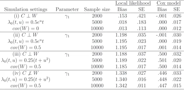
Table 2.1summarizes the simulation results in setting (i)-(iv) with sample sizes 2000,

(31)

Table 2.1: Simulation results of local likelihood in single-index hazards model

Local likelihood Cox model Simulation settings Parameter Sample size Bias SE Bias SE

(i)C ⊥W γ1 2000 .153 .421 -.001 .026

λ0(t, u) = 0.5eut 5000 .018 .183 .000 .017

cov(W) = 0 10000 .013 .113 .000 .012

(ii) C ⊥W γ1 2000 1.198 .035 -.001 .030

λ0(t, u) = 0.5eut 5000 1.195 .023 .000 .019

cov(W) = 0.5 10000 1.195 .017 .001 .014

(iii) C ⊥W γ1 2000 1.188 .037 .500 .032

λ0(t, u) = 0.25(t+u2) 5000 1.189 .022 .501 .020

cov(W) = 0.5 10000 1.185 .017 .500 .014

(iv) C 6⊥W γ1 2000 1.338 .027 .446 .033

λ0(t, u) = 0.25(t+u2) 5000 1.340 .016 .448 .022

cov(W) = 0.5 10000 1.342 .011 .447 .015

NOTE: Each entry is based on 500 replicates.

5000 and 10000, where γ1 is the first component of the γ vector. As expected by

The-orem 2.3.2, the local likelihood approach fails in settings (ii)-(iv) due to the correlation among the vector W and γ0 not being an eigenvector of the covariance matrix of W.

Theorem 2.3.2 also suggests that the local likelihood approach may work in setting (i) because the identity covariance matrix is used. We have also reported the results from

the Cox proportional hazards model. The Cox model produces consistent estimators in

setting (i) and (ii) since the proportional hazards assumption is satisfied, but it gives

biased estimation in setting (iii) and (iv) due to the violation of this assumption.

Figure 2.1 shows the profile local likelihood function based on a simulated data set of size 10000 in each simulation setting. The upper two panels pertain to case (i) and

(ii), respectively; The bottom two panels pertain to case (iii) and (iv), respectively.

The bandwidth is 1×n−1/4_{. Again, the profile local likelihood approach gives biased}

(32)

−1.0 −0.5 0.0 0.5 1.0

1.92

1.93

1.94

1.95

γ1

Profile lik. function

−1.0 −0.5 0.0 0.5 1.0

1.7

1.8

1.9

2.0

2.1

γ1

−1.0 −0.5 0.0 0.5 1.0

1.7

1.8

1.9

2.0

2.1

γ1

−1.0 −0.5 0.0 0.5 1.0

1.55

1.60

1.65

1.70

1.75

1.80

1.85

γ1

Figure 2.1: Profile local likelihood curve of γ1 in single-index hazards model

(33)

2.5 Proofs of Theorems

We denote the second term of (2.5) by (B).

Lemma 2.5.1. If conditions (C1)-(C4) hold, then sup_γ|(B)−1/nPn_j₌₁∆j| →a.s.0.

Proof of Lemma 2.5.1

We partition Γ into small cubes such that any two points in the same cube have

distance no large than δn to be determined later. The number of partitions, denoted by

m∗

n, is of order 1/δqn. Choose one arbitrary point from each of these partitions and denote

them asγ(1)_{, . . . , γ}(m∗

n). For γ

1 and γ2 in the same cube, any fixedy, w,

¯ ¯ ¯ ¯ ¯ 1 nan X

Yj≥y

K

µ

γT

1(Wj−w) an

¶

− 1 nan

X

Yj≥y

K

µ

γT

2(Wj −w) an ¶ ¯¯ ¯ ¯ ¯≤ c a2 n

kγ1−γ2k, and

¯ ¯ ¯ ¯_a1

n E

·

I(Y ≥y)K

µ

γT

1(W −w)

an ¶ ¸ − 1 an E ·

I(Y ≥y)K

µ

γT

2(W −w)

an

¶¸ ¯_¯ ¯

¯≤c1kγ1−γ2k,

for universal constants cand c1. If we choose δn/a2n→0 as n→ ∞, then for any δ >0,

P µ sup γ,y,w ¯ ¯ ¯ ¯_nan1

X

j

I(Yj ≥y)K

µ

γT_(W j −w) an

¶

− 1 anE

·

I(Y ≥y)K

µ

γT_(W ₋_w) an

¶¸ ¯_¯ ¯ ¯> δ

¶

≤P

µ

max

1≤l≤m∗

n sup y,z ¯ ¯ ¯ ¯ ¯ 1 nan X j

I(Yj ≥y)K

Ã

γ(l)T

(Wj−w) an ! − 1 an E "

I(Y ≥y)K

Ã

γ(l)T

(W −w) an !# ¯_¯ ¯ ¯ ¯> δ 2 ¶ ≤ m∗ n X l=1 P µ sup y,z ¯ ¯ ¯ ¯ ¯ 1 nan X j

I(Yj ≥y)K

Ã

γ(l)T

(Wj−w) an ! − 1 an E "

I(Y ≥y)K

Ã

γ(l)T

(W −w) an !# ¯_¯ ¯ ¯ ¯> δ 2 ¶

≤c0m∗nexp(−c1nδ2a2n),

(34)

CDF due to Dvoretzky, Keifer and Wolfowitz (1956). Therefore, ∞ X n=1 P µ sup γ,y,z ¯ ¯ ¯ ¯_na1

n

X

j

I(Yj ≥y)K

µ

γT_(Wj ₋_w) an ¶ − 1 an E ·

I(Y ≥y)K

µ

γT_(W ₋_w) an

¶¸ ¯_¯ ¯ ¯> δ

¶

≤c2

∞

X

n=1

δ−q

n exp(−c1nδ2a2n).

If we choose δn=a3n, then the previous display becomes

c2

∞

X

n=1

a−3q n

ec1nδ2a2n ≤c3

∞

X

n=1

a−3q n (na2

n)m ,

for any positive integer m. Since an = nν1 with ν1 ∈(−1/2,0), we can choose m to be

larger than (1−3qν1)/(1 + 2ν1) such that the previous display is finite. Then, by the

Borel-Cantelli lemma, sup γ,y,w ¯ ¯ ¯ ¯ ¯ 1 nan X

Yj≥y

K

µ

γT_(Wj ₋_w) an ¶ − 1 an E ·

I(Y ≥y)K

µ

γT_(W ₋_w) an

¶¸ ¯¯ ¯ ¯

¯−→a.s. 0.

For any fixed γ, it can be shown that

1 anE

·

I(Y ≥y)K

µ

γT_(W ₋_w) an

¶¸

=E¡I(Y ≥y)|γT_W ₌_γT_w¢_f

γT_W(γTw) +O(a2_n),

where fγT_W(·) is the density function of γTW and O(a2_n) does not depend on y and w.

Hence for any given γ,

sup y,w

¯ ¯ ¯ ¯_an1 E

·

I(Y ≥y)K

µ

γT_(W ₋_w) an

¶¸

−E¡I(Y ≥y)|γT_W ₌_γT_w¢_f

γT_W(γTw)

¯ ¯ ¯

¯−→0.

Note that both 1/anE

h

I(Y ≥y)K

³

γT₍_W_−w₎

an

´i

andE¡I(Y ≥y)|γT_W ₌_γT_w¢_f

γT_W(γTw)

are equi-continuous in γ. Hence,

sup γ,y,w

¯ ¯ ¯ ¯_a1

n E

·

I(Y ≥y)K

µ

γT_(W ₋_w) an

¶¸

−E¡I(Y ≥y)|γTW =γTw¢fγT_W(γTw)

¯ ¯ ¯

¯−→0.

(35)

Therefore, we have proved that sup γ,y,w ¯ ¯ ¯ ¯_na1

n

X

Yj≥y

K

µ

γT_(Wj ₋_w) an

¶

−E¡I(Y ≥y)|γT_W ₌_γT_w¢_f

γT_W(γTw)

¯ ¯ ¯

¯−→a.s. 0.

It then follows that

sup γ ¯ ¯ ¯ ¯ ¯(B)−

1 n n X j=1 ∆j 1 nan n X i=1

I(Yi ≥Yj)K

³

γT₍_W i−Wj)

an

´

E(I(Y ≥y)|γT_W ₌_γT_Wi)_|y₌_Y

jfγTW(γTWi)

¯ ¯ ¯ ¯

¯−→a.s. 0.

Similar arguments can be used to show that

sup γ,y,w ¯ ¯ ¯ ¯ ¯ 1 nan n X i=1

I(Yi ≥y)K

³

γT₍_W i−w)

an

´

E(I(Y ≥y)|γT_W ₌_γT_W

i)fγT_W(γTW_i)

− 1 an

E



 I(Y ≥y)K ³

γT₍_W_−w₎

an

´

E(I(Y ≥y)|γT_W₎_f

γT_W(γTW)

  ¯ ¯ ¯ ¯

¯−→a.s. 0.

Simple calculation shows that the second term inside the absolute value equals 1.

There-fore, sup γ ¯ ¯ ¯ ¯ ¯ ¯ 1 n n X j=1 ∆j 1 nan n X i=1

I(Yi ≥Yj)K

³

γT₍_W i−Wj)

an

´

E(I(Y ≥y)|γT_W ₌_γT_W

i)|y=YjfγTW(γTWi)

− 1 n n X j=1 ∆j ¯ ¯ ¯ ¯ ¯

¯−→a.s.0

and thus sup_γ|(B)−1/nPn_j₌₁∆j| −→a.s.0.

Proof of Theorem 2.3.1

Following the proof for Lemma 2.5.1, we obtain

sup γ ¯ ¯ ¯ ¯ ¯ 1 n X i ∆ilog   1 nan X

Yj≥Yi

K

µ

γT_(W

j −Wi) an ¶  − 1 n X i

∆ilog

¡

E¡I(Y ≥y)|γTW =γTWi

¢

|y=YifγTW(γ

T_W i)

¢¯¯_¯ ¯

(36)

The second term inside the absolute value converges uniformly in γ to

y=YfγT_W(γTW)

¢ª

,

since the involved class of functions is strong P-GC. Therefore,

sup γ

¯ ¯_plloc

n (γ)−plloc(γ)

¯

¯_→_a.s._0.

Proof of Theorem 2.3.2

Note that −∂ ∂γ

¯ ¯

γ=γ0pl

loc_{(γ) equals}

E

"

∆∇γ

¡

E(I(Y ≥y)|γT_W_)f

γT_W(γTW)

¢

E(I(Y ≥y)|γT

0W)fγT

0W(γ

T

0W)

¯ ¯ ¯ ¯

y=Y

#

=EW

· Z

∇γ

¡

E(I(Y ≥t)|γT_W_)f

γT_W(γTW)

¢

E(I(Y ≥t)|γT

0W)fγT

0W(γ

T

0W)

λ0(t, γ0TW)GC(t) exp

¡

−Λ0(t, γ0TW)

¢

dt

¸

=EW

· Z

∇γ¡E(I(Y ≥t)|γT_W_)f

γT_W(γTW)

¢

f_γT

0W(γ

T

0W)

λ0(t, γ0TW)dt

¸

=

Z Z

λ0(y, γ0Tw)fW(w) f_γT

0W(γ

T

0w)

∇γ

¡

E(I(Y ≥y)|γT_W ₌_γT_w)f

γT_W(γTw)

¢

dydw,

whereGC(·) denotes the survival function ofC. The quantity inside the gradient operator

can be written as

lim h→0

1 hE

·

I(Y ≥y)K

µ

γT_W ₋_γT_w h

¶¸

= lim h→0

1 hEW

·

K

µ

γT_W ₋_γT_w h

¶

g(y, γT

0W)

¸

,

where g(y, u) =GC(y) exp (−Λ0(y, u)). Thus

− ∂ ∂γ ¯ ¯ ¯ ¯ γ0

plloc_{(γ) =}

Z Z

λ0(y, γ0Tw)fW(w) f_γT

0W(γ

T

0w)

×lim h→0Eγ0TW

·

1 h2K

0

µ

γT

0W −γ0Tw

h

¶

(E(W|γT

0W)−w)g(y, γ0TW)

¸

dydw.

(37)

Letr(u)≡E(W|γT

0W =u), then the limit inside of the integral is

lim h→0

Z

1 h2K

0

µ

u−γT

0w

h

¶

(r(u)−w)g(y, u)f_γT

0W(u)du

=−g0

2(y, γ0Tw)fγT

0W(γ

T

0w)r(γ0Tw)−g(y, γ0Tw)fγ0T

0W(γ

T

0w)r(γ0Tw)

−g(y, γT

0w)fγT

0W(γ

T

0w)r0(γ0Tw) +g02(y, γ0Tw)fγT

0W(γ

T

0w)w+g(y, γ0Tw)fγ0T

0W(γ

T

0w)w,

where g0

2(y, u) = ∂u∂ g(y, u). Hence, the double integral equals

Z

EW

·

λ0(y, γ0TW)

µ

−g₂0(y, γ₀TW)r(γ₀TW)−g(y, γ₀TW)f 0 γT

0W

f_γT

0W

(γ₀TW)r(γ₀TW)

−g(y, γT

0W)r0(γ0TW) +g20(y, γ0TW)W +g(y, γ0TW)

f0 γT

0W

f_γT

0W

(γT

0W)W

¶¸

dy

=−

Z

E_γT

0W

¡

λ0(y, γ0TW)g(y, γ0TW)r0(γ0TW)

¢

dy.

Since W ∼N(µ,Σ), r0_{(u) = (γ}T

0Σγ0)−1Σγ0 for any u. Thus the last display becomes

−(γT

0Σγ0)−1Σγ0

Z

E_γT

0W

¡

λ0(y, γ0TW)g(y, γ0TW)

¢

dy=−E[∆](γT

0Σγ0)−1Σγ0.

By (C6), E[∆] > 0. Thus the display is proportional to γ0 if and only if Σγ0 ∝ cγ0 for

(38)

Chapter 3 Partly Proportional Single-Index

Hazards Model

3.1 Model and Data Structure

In this chapter, we assume the following partly proportional single-index hazards (PPSIH)

model

h(t|X, Z) =λ(t, γTZ)eβTX, (3.1)

where β ∈ Rp_{, γ} _∈ _Rq _and _λ(·,_{·) is an unknown bivariate function. When} _γ _{is a} con-stant and Z is one dimensional, (3.1) reduces to a special case of the model studied by

Dabrowska (1997). When β is zero or there is no X, (3.1) reduces to the single-index model proposed in Chapter2. To ensure identifiability of this model, we first impose the restriction that kγk = 1 with the last coordinate γq of γ positive, that is, γ is restricted to the half unit sphere. This assumption is practically reasonable when at least one

“nuisance” covariate has a non-zero effect. Other identifiability and regularity conditions

are given in Sections 3.2 and 3.3.

The single-index hazards model