TESTING-BASED COMMUNITY DETECTION METHODS FOR COMPLEX NETWORKS
John J. Palowitch
A dissertation submitted to the faculty of the University of North Carolina at Chapel Hill in partial fulfillment of the requirements for the degree of Doctor of Philosophy in the Department
of Statistics and Operations Research.
Chapel Hill 2017
ABSTRACT
JOHN J. PALOWITCH: Testing-Based Community Detection Methods for Complex Networks
(Under the direction of Andrew B. Nobel)
Community detection is an exploratory method of grouping strongly connected nodes in a net-work, in most cases using only the network edge structure as a guide. Using discovered communities for downstream analyses can be crucial for real-world decision-making and inference. Recent ap-proaches to community detection include testing-based community extraction, a process in which communities are refined one-by-one via analysis of graph statistics. However, to date, testing-based extraction methods are tied to the configuration model as a null, which applies only to single-layer, binary graphs.
In this thesis, testing-based extraction is generalized to arbitrary networks types with a frame-work called Node-Set Testing (NST). The NST frameframe-work defines the broader statistical elements of an approach that uses hypothesis testing to detect communities in complex networks. The NST framework is applied to (i) weighted networks and (ii) bipartite correlation networks, resulting in novel community detection algorithms. In particular, new null models and test statistics are speci-fied to apply iterative hypothesis-testing algorithms on these types of networks. Detailed analyses of the empirical and theoretical properties of the proposed methods are provided.
Other chapters in this thesis, while not explicitly involving testing-based algorithms, support the discussion of community detection in heterogeneous networks. One chapter provides a consis-tency analysis of a significance-based score for community extraction in multilayer networks. In another chapter, preceding the discussion of the NST method for bipartite correlation networks, an application area called eQTL analysis is discussed. In particular, a new model for estimating the effect size and regression correlation of the links in an eQTL network is introduced and studied.
To Marilyn Maiden Palowitch and Carl Joseph Palowitch, my parents; to whom I attribute my curiosity, dedication, and enthrallment with understanding;
ACKNOWLEDGEMENTS
I have an enormous amount of gratitude for my collaborators and their professional and personal contributions to the work presented in this thesis. First and foremost, I thank my advisor Dr. Andrew B. Nobel. Dr. Nobel’s near-endless energy and enthusiasm, combined with a genuine regard for and honest criticism of all my ideas, created an environment in which my needs for creative exploration and rigorous training were well-satisfied. I also thank my secondary advisor Dr. Shankar Bhamidi. Dr. Bhamidi continually challenged me to think more intuitively about complex problems, and provided me with fantastic advice about the relationships between research directions, career goals, and life endeavors.
I thank Dr. James S. Marron for a year’s worth of immersion in his diverse and interesting research directions. I thank Dr. Perry Haaland under whom I worked a semester-long internship at Becton-Dickinson in Research Triangle Park. My collaboration with Dr. Marron and Dr. Haaland was an indispensable part of my growth as a statistician and data scientist. I am especially grateful for the presence of Dr. Peter J. Mucha and Dr. Yufeng Liu on my committee, as Dr. Mucha is technically on sabbatical this semester, and Dr. Liu is a new parent (congratulations!). Over the past year, I have met with Dr. Mucha and one of his postdoctoral researchers Dr. Dane Taylor to discuss interesting new directions in network science: I have greatly appreciated these conversations. A large chapter in this thesis is devoted to my work on the Genotype Tissue Expression (GTEx) project. Along with Dr. Nobel, the other P.I. on our working group was Dr. Fred A. Wright, the Director of the Bioinformatics Research sCenter at NCSU. Dr. Wright’s approach to research was a continual source of inspiration. His ways of thinking about modeling and significance were (and remain) formative to my statistical intuitions. Also in our working group was Dr. Andrey Shabalin, assistant professor at VCU. Dr. Shabalin was the main contributer to the software implementations of our new eQTL model, and was an indispensable collaborator in the refinement of the model’s theoretical underpinnings. I am grateful for the opportunity to have worked alongside Andrey, as his experience and advice greatly improved my ability to think systematically about programming
TABLE OF CONTENTS
LIST OF TABLES . . . xiii
LIST OF FIGURES . . . xiv
LIST OF ABBREVIATIONS AND SYMBOLS . . . xvi
1 Introduction . . . 1
1.1 Preliminary Notation . . . 4
1.2 Fundamental work on community detection . . . 5
1.2.1 The Stochastic Block Model . . . 5
1.2.2 The configuration and Chung-Lu models . . . 6
1.2.3 Modularity and optimization . . . 9
1.2.4 Spectral clustering . . . 10
1.3 Recent directions in community detection . . . 11
1.3.1 Community Extraction . . . 11
1.3.2 The Degree-Corrected Stochastic Block Model . . . 12
1.3.3 Consistency of community detection methods . . . 14
1.3.4 Community detection for multilayer and bipartite networks . . . 16
1.3.4.1 Bi-partite networks . . . 17
1.4 Contributions of this thesis . . . 18
1.4.1 Community extraction for edge-weighted networks . . . 19
1.4.2 Community extraction for multi-layer, binary networks . . . 20
1.4.3 eQTL analyses and bi-partite correlation networks . . . 21
1.5 Document Organization . . . 23
2 Node-Set Testing for Complex Networks . . . 24
2.2 Node-set association testing . . . 26
2.3 The Stable Community Search (SCS) algorithm . . . 28
2.4 Background and Type-I Error . . . 30
2.4.1 Global Error Control . . . 31
2.4.2 Discussion . . . 32
3 Continuous Configuration Model Extraction . . . 35
3.1 Notation and terminology . . . 35
3.2 The continuous configuration model . . . 36
3.2.1 Model statement . . . 37
3.2.2 Null specification of the model . . . 38
3.3 Test statistic and theoretical results . . . 39
3.3.1 A test statistic for node-set association in weighted networks . . . 39
3.3.2 Asymptotic Normality ofS(u, B,G) . . . 41
3.3.3 Consistency of SCS . . . 42
3.3.3.1 The weighted stochastic block model . . . 42
3.3.3.2 Consistency theorem . . . 43
3.3.3.3 Connection to weighted modularity and related work . . . 47
3.4 The Continuous Configuration Model Extraction algorithm . . . 47
3.4.1 Step 1: Initialization . . . 48
3.4.2 Step 3: Filtering ofC. . . 49
3.5 Simulations . . . 49
3.5.1 Performance measures and competing methods . . . 49
3.5.2 Simulation settings and results . . . 50
3.5.2.1 Networks with varying signal levels . . . 51
3.5.2.2 Networks with overlapping communities . . . 52
3.5.2.3 Networks with overlapping communities and background nodes . . . 52
3.6.1 U.S. airport network data . . . 54
3.6.2 ENRON email network . . . 54
3.7 Discussion . . . 56
4 Multi-layer Community Extraction . . . 58
4.1 Significance-based scoring of a vertex-layer group . . . 58
4.1.1 The Null Model . . . 59
4.1.2 Multilayer Extraction Score . . . 60
4.2 Consistency Analysis . . . 61
4.2.1 The Multilayer Stochastic Block Model . . . 61
4.2.2 Consistency of the Score . . . 62
4.2.2.1 Consistency of the joint optimizer . . . 64
4.2.3 Proofs . . . 65
4.2.3.1 Proof of Theorem 11, and Supporting Lemmas . . . 66
4.2.3.2 Sketch of the Proof of Theorem 11 . . . 66
4.2.3.3 Supporting lemmas for the Proof of Theorem 11 . . . 67
4.2.3.4 Proof of Theorem 11 . . . 70
4.2.3.5 Proof of Theorem 12 . . . 71
4.3 The Multilayer Extraction Procedure . . . 72
4.3.1 Initialization . . . 73
4.3.2 Extraction . . . 73
4.3.3 Refinement . . . 74
4.3.3.1 Choice ofβ . . . 75
4.4 Discussion . . . 76
5 Bipartite Correlation Networks . . . 77
5.1 The ACME-eQTL model for eQTL effect size . . . 77
5.1.1 Existing approaches to gene expression modeling . . . 77
5.1.2 Framework and notation . . . 78
5.1.3 The ACME-eQTL model and diagnostics . . . 79
5.1.3.1 Log ANCOVA and log-linear models . . . 80
5.1.3.2 Model statement . . . 81
5.1.3.3 Model fit diagnostics . . . 82
5.1.4 Modelp-values and Type I error . . . 84
5.1.4.1 Empirical performance of theF test . . . 85
5.1.5 Power, estimation accuracy, and computation speed . . . 86
5.1.5.1 Computation times . . . 87
5.1.6 Large-scale real data analysis . . . 89
5.1.7 Discussion . . . 91
5.2 Future work: Bi-community detection for correlation networks . . . 92
5.2.1 The NST Framework for Bi-partite Networks . . . 92
5.2.2 Notation and CBCE Framework . . . 94
5.2.3 SCS test statistic and p-value for bi-partite correlation networks . . . 94
5.2.4 The CBCE method . . . 96
5.2.5 Simulation results . . . 97
5.2.5.1 Simulation model . . . 98
5.2.5.2 Performance measures . . . 99
5.2.5.3 Competing methods . . . 101
5.2.5.4 Simulation settings and results . . . 102
5.2.6 Conclusion . . . 104
5.3 Acknowledgements . . . 104
6 Future Work and Conclusion . . . 106
Appendix A NODE-SET TESTING SUPPLEMENTAL . . . 108
A.1 Cycles in Fixed Point Search . . . 108
A.2 Proof of Theorem 4 . . . 108
B.1 Proof of Proposition 5 . . . 111
B.2 Filtering ofB0 and C . . . 111
B.3 Simulation Framework Preliminaries . . . 112
B.4 Simulation of community nodes . . . 112
B.4.1 Community structure and node degree/strength parameters . . . 113
B.4.2 Simulation of edges and weights . . . 114
B.4.3 Parameter settings . . . 114
B.5 Background node simulation . . . 115
B.5.1 Adjusted community-node simulation model . . . 116
B.5.2 Edges and weights for background . . . 116
B.6 Proof of Theorem 6 and supporting lemmas. . . 118
B.6.1 Completing the proof of Theorem 6. . . 124
B.7 Proof of Theorems 8-9 and supporting lemmas. . . 124
B.7.1 Proof of Lemma 8 from the main text . . . 130
B.7.2 Proof of Theorem 9 from the main text . . . 137
Appendix C MULTI-LAYER EXTRACTION SUPPLEMENTAL . . . 142
C.1 Proof of Lemma 15 . . . 142
C.2 Proof of Lemma 16 . . . 143
C.3 Proof of Lemma 18 . . . 146
C.4 Proof of Lemma 21 . . . 147
C.5 Technical Results . . . 148
Appendix D ACME SUPPLEMENTAL . . . 158
D.1 Pre-processing gene read counts . . . 158
D.2 Sampling scheme for residual and goodness-of-fit tests . . . 158
D.3 Framework for direct null simulation . . . 158
D.4 Tests of normality and homoskedasticity . . . 159
D.5 QN-linear regression vs. ACME-eQTL regression . . . 160
LIST OF TABLES
3.1 Metrics from methods’ results on ENRON network: number of communities, minimum community size, median community size, maximum community size,
count of nodes in any community . . . 56
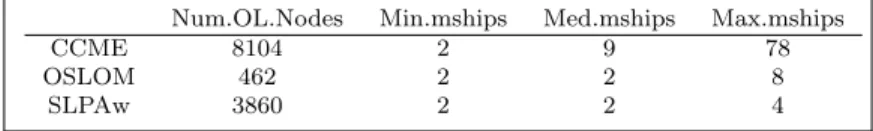
3.2 Metrics from methods’ results on ENRON network: number of overlapping nodes, minimum # of memberships, median # of mem’ships, max. # of mem’ships . . . 56
3.3 Top domains associated with community nodes from each method, by proportion . . . 56
5.1 Simulation model parameters . . . 98
LIST OF FIGURES
1.1 Two-hundred high-degree nodes from a network formed by data from the Lit-tleSis website, which tracks powerful people and their business and political connections. Edges are placed and weighted according to output from a
non-parametric bayesian model with similarities to the SBM (Kim et al., 2013). . . 7 1.2 The configuration model applied to an empirical random network. Source:
Aaron Clauset’s CSCI5352 lecture notes, Sante Fe Institute. . . 9 1.3 Visualization of a political blog network, labels estimated by the standard SBM
(a) and the DCSBM (b) (Newman, 2012). . . 14
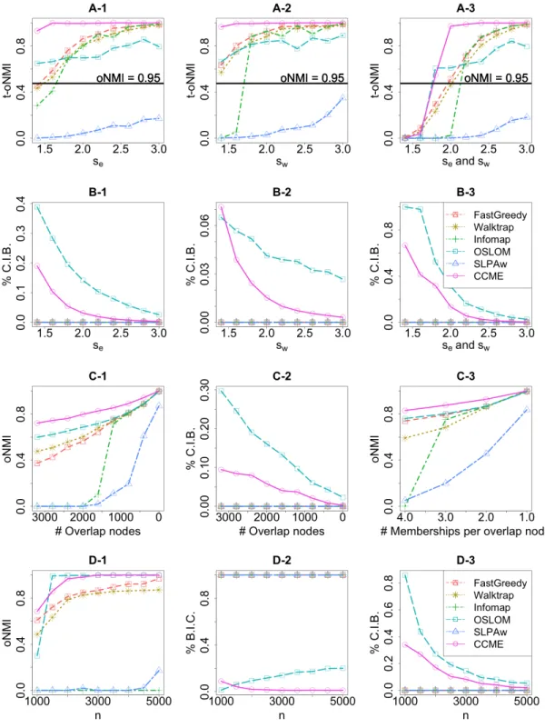
3.1 Simulation results described in Sections 3.5.2.1-3.5.2.3. Legends correspond to
all plots. . . 53 3.2 SLPAw, OSLOM, and CCME results from June 2015 and 2015-year-aggregated
U.S. airport networks. Maps created with ggmap(Kahle and Wickham, 2013) . . . 55
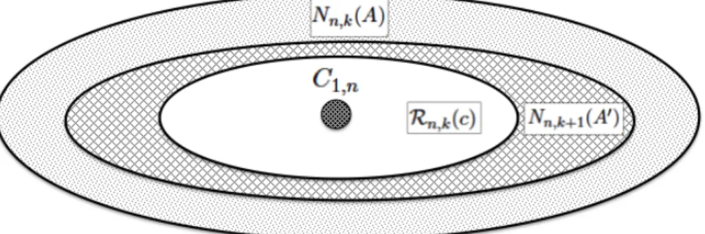
4.1 Illustration of relationship between collections of node sets. . . 69
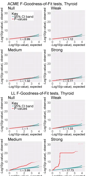
5.1 Q-Q plots of likelihood ratio test p-values for ACME-eQTL and log-linear models, in each sector of GTEx Thyroid sample data, n= 105. The grey line is where we would expect thep-values (represented by the red dots) to fall if they were perfectly uniform, and the green line represents the 95% window of
error around this expectation. λis the estimated genomic inflation factor. . . 85 5.2 p-value distributions from null simulated data with realistic errors and real
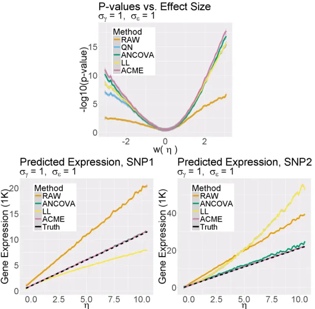
covariate/genotype data. λvalues are inflation factors. . . 86 5.3 Results of large-scale simulation experiment. Left: −log 10 F-test p-values as
a function ofη. Middle and right: predicated raw expression with one and two
reference alleles, respectively. . . 88 5.4 Results of genome-wide cis-eQTL ACME effect size estimations on Thyroid
tissue (n = 105), from GTEx Pilot data. Bottom-left: Maximum gene-wise estimated effect size vs. log average expression level. Top-left: F p-values from the QN-linear model vs.F p-values from the ACME-eQTL model. Top-right: −log10 ACME-eQTL p-value vs. distance from gene TSS to SNP position. Bottom-right: Full-tissue procedure times of the Matrix-EQTL and
ACME-eQTL fitting softwares. . . 90 5.5 Correlation matrix ofX from a draw from the default simulation model. . . 100 5.6 Simulation model instances with varyingµβ (betamean). . . 103
5.8 Simulation model instances with varyingg (“bgmult”). . . 104
B.1 Empirical degrees/strengths vs. adjusted parameters for the example network . . . 118 B.2 Average empirical z-statistics between nodes and node blocks . . . 119 B.3 SLPAw, OSLOM, and CCME results from January and Februrary 2015 U.S.
airport networks. Maps created withggmap(Kahle and Wickham, 2013) . . . 139 B.4 SLPAw, OSLOM, and CCME results from March and April 2015 U.S. airport
networks. Maps created with ggmap(Kahle and Wickham, 2013) . . . 140 B.5 SLPAw, OSLOM, and CCME results from May and July U.S. airport networks.
Maps created withggmap (Kahle and Wickham, 2013) . . . 141
D.1 Boxplots of−log10Shapiro-Wilk and Bartlettp-values from all models. Above, “AOV” denotes the log-ANCOVA model, “LL” the log-linear model, and “RAW” the standard linear model with un-transformed gene expression. The dark red dashed line indicates the FDR α = 0.1 significance cut-off for the
particular bin. . . 160 D.2 eQTL data from two selected gene-SNP pairs from Adipose tissue. The fitted
lines correspond to the estimated parameters from each model. . . 161
LIST OF ABBREVIATIONS AND SYMBOLS
n
[b]
u, v
C
A
G
v(u)
vT
d
W
s
NST SCS
SBM, DCSBM CCME
ACME-eQTL
Sample size of a network or Euclidean data set. For a positive integer b, the index set [b] := 1, . . . , b. Indices for nodes, e.g. u, v∈[n].
A node-set cover: C:={C1, . . . , CK} withCj ⊂[n] for allj ∈[K]. Adjacency matrix. A[u, v] = 1 if and only ifu and v are connected. A networkG = ([n], A).
The u-th component of an n-vectorv
Denotes the vector sum of v, definedvT :=
P
u∈[n]v(u). The vector of node degrees, where d(u) :=P
v∈[n]A[u, v]. For weighted networks, the adjacency matrix of weights. The vector of node strengths, wheres(u) :=P
v∈[n]W[u, v]. Node-Set Testing
Stable Community Search
(Degree-Corrected) Stochastic Block Model Continuous Configuration Model Extraction
CHAPTER 1
Introduction
A network can be both a mathematical structure, having an abstract set of nodes and edges, and a natural phenomenon, consisting of objects and their interactions. Sometimes there is, in some sense, an isomorphism between a physical network and its mathematical representation. Road networks, electric networks, and internet networks all have a set of physical, fixed nodes and links that can be identified with a binary graph. Analyses of these networks often involve questions about logistics and operations, like finding efficient ways to schedule travel routes, packet transfers, or computing jobs.
Most often, however, natural systems are only represented by a mathematical network. For instance, a gene interaction network is a set of genes and their regulatory relationships. The exis-tence of such networks are acknowledged through a build-up of statistical evidence for correlations between genomic regions. However, gene networks do not necessarily correspond to biophysical pathways. In general, networks that represent a system are studied in a more scientific manner. Nodes are treated as data objects, and their emergent relationships seen as stochastic, potentially indicative of underlying group dynamical structure in the system under analysis.
The topics in this thesis focus on the scientific and statistical analysis of real-world systems through network data objects. In particular, the statistical methods this work introduces apply to complex networks. The term “complex network” initially arose when natural networks of interest became large and quite unlike standard random graph models of the mid-to-late twentieth century. Hence, the study of complex networks is defined by a focus on large-scale, heterogeneous properties of networks, like topology, clustering, and degree distributions (Albert and Barab´asi, 2002).
Still others have hierarchical levels of sub-networks. Each separate data attribute in a network carries rich information of potential import to any analysis question (Boccaletti et al., 2006). As such, methods introduced in this thesis will have a particular focus on networks with more-than-one type of network data.
Myriad descriptions of studies involving networks with more than one attribute are given in the aforementioned references; here are just a few more notable examples:
1. Almaas et al. (2004) studied the molecular reaction network of theE. coli metabolism, with edges weighted by the reaction fluxes, providing deeper insights into bacterial metabolic organization and regulation.
2. Barrat et al. (2004) analyzed the collaboration network of authors contributing to the condensed-matter physics electronic archive between 1995 and 1998. The network contained
n = 12,722 authors, with edges weighted by number of collaborations. Their analysis re-vealed, quantitatively, some intuitive findings about the relationship between academic col-laborativestructureandvolume, for instance that highly published authors produce a plurality of their total output with a stable research group.
3. Ansari et al. (2011) developed flexible parametric models for multi-layer networks. In their work, they analyzed network data from a Swiss social media platform that connects musi-cians with listeners as well as with other musimusi-cians. The network data had three layers, each with different attributes: a binary, undirected friendship layer; a binary, directed messag-ing layer; and a weighted, directed music downloadmessag-ing layer. They showed that modelmessag-ing diverse attributes separately, accounting for specific data types, greatly improved predictive performance.
systems biology, life sciences, marketing, and computer science (cf. Palla et al. (2007); Barabasi and Oltvai (2004); Lusseau and Newman (2004); Guimera and Amaral (2005); Reichardt and Bornholdt (2007a); Andersen et al. (2012)). Surveys of the network science and methodology literature have been provided by Newman (2003b) and Jacobs and Clauset (2014), among others.
The primary, specific focus of this dissertation is community detection methods for complex networks, in particular networks with data attributes beyond binary edges. A common, loose definition of a community is a subset of nodes that are more connected internally than externally. Community detection is one of the most important network analysis techniques, as communities often reflect intrinsic structure of the system the network represents. Finding communities among objects of study in a data set can support exploratory analysis and provide an important starting point for further scientific inquiry or decision-making (Danon et al., 2005). For example:
1. Hundreds of studies in computational biology have used community detection to find subsets of genomic loci, genes, cells, or micro-organisms with high levels of interaction. These subsets can be focal points for a variety of downstream analyses, and can spur new insights about the underlying mechanics of genomes (Chen and Yuan, 2006; Cabreros et al., 2015; Platig et al., 2015; Fan et al., 2012).
2. Community detection has been used to facilitate recommender systems in online social net-works: first by grouping users through their observed edge (or edge weight) interactions, and then by suggesting interests of users to the rest of their group (Sahebi and Cohen, 2011; Xin et al., 2014).
3. To study buyer patterns on eBay, community detection was used to group bidders based on common bidding interests (Reichardt and Bornholdt, 2007b) and to group auctions based on common bidders (Jin et al., 2007). The latter analysis, in particular, was used to predict and recommend equally valuable auction items to bidders (Fortunato, 2010).
Countless other examples of community detection applications can be found in surveys by Porter et al. (2009), Fortunato (2010), and Fortunato and Hric (2016), and the references therein.
Most standard community detection methods involve the optimization of a quality function for network partitions. For some methods, the quality function is a log-likelihood; for other methods,
it is a more general score of the intra-connectedness and inter-disconnectedness of the partition’s elements. Various quality functions will be discussed in more detail in Section 1.2. Optimization approaches to community detection have proven extremely effective for decades, in countless ap-plications. However, the results of these methods rarely come with a significance guarantee or statistical interpretation. Basic simulations will show that many commonly-used community de-tection methods reliably find communities in networks that (arguably) lack community structure.
This thesis introduces and analyzes applications of a testing-based framework to community detection on networks with (potentially) multiple data types. The framework re-motivates com-munity detection from a statistical testing perspective, providing an iterative hypothesis-testing algorithm for the discovery of significantly associated node sets. This approach is contrasted with optimization-based community detection, an approach which (in general) does not provide guarantees of statistical significance. As the major components of the work presented here, new testing-based algorithms are derived for various types of networks. Illustrations of these methods’ advantages, empirical efficacies, and theoretical results regarding consistency and error control are provided. In Section 1.4, more introductory detail is provided about these contributions. The sections below provide an in-depth review of existing community detection methodology.
1.1 Preliminary Notation
I denote a general network object with n nodes by G := ([n],D), where [n] = 1, . . . , n is the node set, andDis a data object which encodes the observed interactions between nodes. We callG a “binary” or “un-weighted” network whenDis a matrixA∈ {0,1}n×ncontaining edge indicators. Explicitly, letu, v∈[n] be general node indices, and letA[u, v] denote theu, v-th entry ofA, which equals 1 if and only if u and v share an edge. Unless otherwise specified, we assume thatA[u, v] is symmetric and that A[u, u] = 0 for all u ∈ [n]. A partition of a node set is a finite collection
C1, C2, . . . , CK ⊆[n] such that∪iCi= [n] and Ci∩Cj =φfor alli6=j. In other words, each node is assigned to exactly one community. Usually, a partition will be denoted with the concise vector representation c∈ [K], with elements c(u) giving the community assignment of u. We define the degree of nodeu∈[n] byd(u) :=P
The “total” degree is defined dT := Pu∈[n]d(u). Note that for undirected binary graphs, dT is simply twice the number of edges in the graph.
1.2 Fundamental work on community detection
Community detection is a wide and varied and field of research, with plentiful and sub-sub-fields. In what follows, I give a brief overviews of some classical theoretical and methodological directions in the study of communities in networks.
1.2.1 The Stochastic Block Model
Real-world interconnected systems have been studied with tools from network science and graph theory since the early twentieth century. Particularly in social science and biology, it eventually became common to view densely-connected subregions of a graph as emergent macro-structure in the system of scientific interest. Early on, Holland et al. (1983) and Anderson et al. (1992) proposed the Stochastic Block Model (SBM) as one way to model macro-structure in a networked system. In the model, nodes are organized into disjoint “blocks” with diverse intra- and inter- connection probabilities. The blocks represent meaningful real-world node subgroups which potentially interact at different rates within-block than out-block. Snijders and Nowicki (1997) gave both maximum likelihood and Bayesian approaches to estimating both the block structure and the connection probabilities for a 2-block SBM, though they soon generalized their procedure in Nowicki and Snijders (2001). The SBM approach to community detection has been of instrumental importance to the social and biological sciences (Fortunato, 2010; Porter et al., 2009).
Variants of the SBM will be of central focus in parts of this thesis. As such, an explicit definition of the model is now provided. The SBM is a generative stochastic model for an undirected, binary graph G:= ([n], A), with three parameters. The first parameter is the number of communities (or blocks)K. The second is a community partition vector c, where c(u)∈[K] gives the community index ofu. The third parameter is aK×K probability matrixP. In the model, an edge is placed between nodesu and v (independently of all other edges) with probability
puv=P[c(u), c(v)]. (1.1)
Thus, the indicator1{A[u, v] = 1}is Bernoulli(puv), and the resulting networkG = ([n], A) has the likelihood
L(G|K,c,P) := Y 16u<v6n
pAuv[u,v](1−puv)1−A[u,v] (1.2)
The model can be seen as a generalization of an Erd˝os-R´enyi network, inducing community structure throughcand the matrixP. The most common type of community structure of interest, in usual applications, is when the diagonals of P are larger than the off-diagonals. In the model, this will cause nodes to connect more frequently to other nodes in their community, on average, than to nodes outside their community. This is usually called “assortative” community structure. Figure 1.1 shows an example of a network exhibiting strong assortative community structure (Kim et al., 2013). The estimated SBM for this network would have K = 4 or 5 blocks, large diagonal entires of P, and off-diagonal entries of P near zero. The SBM is, of course, equally capable of generatingdisassortive structure, in which nodes connect more frequently outside their community, a pattern which can also be of interest (Aicher et al., 2014). The SBM has since been extended to include overlapping nodes (Whang et al., 2013; Airoldi et al., 2009), directed edges (Latouche et al., 2011), and heterogeneous expected degrees (as will be covered in Section 1.3.2). Aicher et al. (2014) provided a weighted version of the stochastic block model in which edge weights are random variables from an exponential family.
An important sub-field of network analysis regards the latent space model (Hoff et al., 2002), which has close ties to the SBM. In the latent space model, nodes are assumed to have unobserved positions in an underlying metric space. The distance to other nodes in the metric space govern their observed interactions in the network. Some fundamental similarities between the latent space model and the stochastic block model were discussed in Rohe et al. (2011). Compared with other models and methods discussed in this work, Bayesian techniques play a much more prominent role in standard applications of latent space models (Sarkar and Moore, 2005).
1.2.2 The configuration and Chung-Lu models
Figure 1.1: Two-hundred high-degree nodes from a network formed by data from theLittleSis website, which tracks powerful people and their business and political connections. Edges are placed and weighted according to output from a nonparametric bayesian model with similarities to the SBM (Kim et al., 2013).
sequence d = {d(1), . . . , d(n)}, with d(u) 6 n for all u ∈ [n]. Initially, the configuration model was introduced in context of the general study of random graphs and their distributional proper-ties (Bollob´as, 1980; Bender, 1974). Molloy and Reed (1995) gave an algorithm for generating the configuration model, which can be written as follows:
1. Form a setL of half-edges, withd(u) half-edges assigned to each node u∈[n].
2. Draw two half-edges uniformly-at-random fromL, without replacement; form an edge. 3. Repeat step 2, always without replacement, until all half-edges are exhausted.
Note that this process generates an undirected graph, and thus dT must be even. This process also allows for “self-loops” (A[u, u] = 1) and multiple edges. However, easy modifications of the algorithm can prohibit these features.
A model that is closely related to the configuration model is that of Chung and Lu (2002). Given a degree sequence d, the model is generated by placing an edge between nodes u and v,
independently of all other edges, with probability
puv= min
d(u)d(v)
dT
, 1
, (1.3)
where dT is the total degree (see Section 1.1). This “Chung-Lu” or “Expected-Degree Random Graph” model, as it is often called, is more directly related to the Erd˝os-R´enyi model than the configuration model, since it retains edge-independence. In fact, whereas with the configuration model the sequence d is best seen as a restriction on the Erd˝os-R´enyi, in the Chung-Lu model it is a generalization. When all degrees are equal to some fixed d, the Chung-Lu model reduces to Erd˝os-R´enyi with probabilityd/n. Nonetheless, fundamental and important similarities remain between the Chung-Lu and configuration models. It is easy to derive that, if maxuvd(u)d(v)6dT, the expected degrees under the Chung-Lu model are precisely d. Conversely, when dT =o(n), the probability of an edge betweenu and v under the configuration model is approximately puv.
Though neither the configuration nor Chung-Lu models were originally introduced in the con-text of community detection, they eventually played important (and related) roles in the study of communities. Newman et al. (2002) published an early, often-cited paper proposing the utility of the configuration model for simulating social networks. They noted the inadequacy of Erd˝os-R´enyi networks for this task, as the degree-distribution of real-world networks are always skewed. Notably, Newman writes that the configuration model produces “a graph with exactly the desired degree distribution, but which is in all other respects random”. This may be the first acknowledgment (albeit implicit) that the configuration model may be a suitable null model to test for alternative structure in graphs with heterogenous degrees. Indeed, soon after that publication, community detection methods based on the 1st-order structure in the configuration and Chung-Lu model were introduced, as discussed in the next section. These new methods fundamentally changed the field, and the related roles of the configuration and Chung-Lu models in these research directions are now well-known (Olhede and Wolfe, 2012; Durak et al., 2013).
configura-Figure 1.2: The configuration model applied to an empirical random network. Source: Aaron Clauset’s CSCI5352 lecture notes, Sante Fe Institute.
tion model algorithm to an empirical network can be thought of as a permutation of the edges, conditional on the observed degrees. Significance of the community structure in the observed net-work can therefore be assessed either by successive applications of the model algorithm, in the style of a permutation test, or by analysis of test statistics from the network with respect to the distribution of the model.
1.2.3 Modularity and optimization
A novel approach to community detection was introduced via themodularitymetric by Newman and Girvan (2004). Modularity is a score of a network partition such that, loosely speaking, when it is large, the community structure given by the partition is strong. The modularity score compares the empirical edge densities to the expected edge densities under the configuration model (see Section 1.2.2). Explicitly, the modularity score sums the difference between edge indicators of node pairs in the same community from their corresponding Chung-Lu probability puv (see Equation 1.3). Given a network partition c, modularity is defined
Q(c) := 1
dT
X
u,v∈[n]
A[u, v]−d(u)d(v)
dT
1(c(u) =c(v)), (1.4)
where 1 is the indicator function. Note that Q(c) is always in the interval [−1,1]. From the above equation, it is obvious that when the edge densities within the communities outlined by the partition c are much larger than what is expected under the configuration model, Q(c) will be closer to 1.
Finding the global maximizer of modularity is NP-complete (Brandes et al., 2006). Thus, all commonly-used community detection methods based on modularity employ approximation algo-rithms. Girvan and Newman gave the first approach to approximately maximizing modularity, which involves first an edge-removal algorithm for finding proposed partitions (Girvan and New-man, 2002), then a method to choose a partition using the modularity score (Newman and Girvan, 2004). Modularity-based methods have been generalized, re-worked, and analyzed in many ways over the years (Newman, 2004b, 2006b; Clauset et al., 2004; Eriksen et al., 2003; Langone et al., 2011), and now are among the most popular tools in network science. The modularity score has also been extended to networks with directed edges and overlapping communities (Nicosia et al., 2009; Chen et al., 2014), and to networks with bipartite community structure (Barber, 2007), as will be discussed more fully in Section 1.3.4. Overall, the modularity approach represents a marked departure from the model-based community detection procedures described in Section 1.2.1.
Importantly, the modularity framework is not the only approach to assessing or finding com-munity partitions in networks. Pre-dating modularity, the conductance measure of a node set is the ratio of cross-edges between that set and its complement to the number of internal edges of the set. A thorough study of conductance and how it has been used to detect communities, including novel approaches, is given by Leskovec et al. (2008). Other partition-based community detection methods have roots in information theory or random walks. These methods involve many diverse approaches to community detection and types of algorithms. Three examples are: (i) Infomap (Rosvall and Bergstrom, 2008), an algorithm incorporating information-theoretic measures of com-munity structure; (ii) Walktrap (Pons and Latapy, 2005), an algorithm incorporating random walk probabilities; and (iii) a label-propagation algorithm presented in (Raghavan et al., 2007). These methods perform quickly even for large networks and have been implemented in standard software packages fromRand python, making them commonly used tools in applied network science.
1.2.4 Spectral clustering
detection are in the graph partitioning work of the mid-to-late twentieth century. One early and particularly influential paper in this field called “Algebraic connectivity of graphs” was written by Miroslav Fiedler (1973). In that paper, Fiedler relates the eigenvalues of an unweighted, undirected network’s adjacency matrix to its connectedness. Much subsequent, related work analyzed further relationships between graph spectra and optimal cuts of the graph using linear algebra and theory of random walks (Ding et al., 2001; Pothen et al., 1990). While these results are most directly applied to problems in (for example) distributed computing and circuit designs (Chamberlain et al., 1998; Shirinivas et al., 2010), they laid the groundwork for the spectral approach to clustering and community detection (Boccaletti et al., 2006). Some examples of the application and analysis of spectral approaches to community detection can be found in (for example) Newman (2006a,b); Richardson et al. (2009); Rohe et al. (2011); Newman (2013).
1.3 Recent directions in community detection
In recent years, the field of community detection has expanded to include novel algorithmic ap-proaches, nuanced theoretical analyses, and additional methods for new types of complex networks. Current directions that pertain to the work in this thesis are now discussed.
1.3.1 Community Extraction
The classical approaches to community detection described in Section 1.2 are all based on the evaluation of a community partition. An alternative approach is to conduct set-wise searches, in which communities are identified and evaluated one-by-one. This approach, often called community “extraction”, can feature a number of attractive benefits. One particular benefit is that not all nodes need to be assigned a community. Usually, this happens for nodes that do not have strong connectivity to any other subgroup. In this work, I such nodes are called “background”. Extraction methods have been put forth in a number of recent publications:
1. For a community C⊆[n], Zhao et al. (2011) defined the following measure of connectivity:
Q(c) :=|C|−1
|C|−1 X
u,v∈C
A[u, v]− |Cc|−1 X u∈C,v∈Cc
A[u, v]
.
The above measure compares the average in-degree of C to the average out-degree. Though this measure is fundamentally heuristic and model-free, it captures a reasonable conception of empirical community strength. Zhao et al. (2011) give a node-swapping algorithm to locally maximize this metric over all possible node sets. Though their algorithm can identify background, one of its drawbacks is that overlapping communities are dis-allowed.
2. Lancichinetti et al. (2011) introduced the Order Statistics Local Optimization Method (OSLOM), which locally optimizes a “fitness” function characterizing the statistical signifi-cance of a community with respect to the configuration model. Their algorithm is capable of handling networks with directed and weighted edges, can detect hierarchical community structure, and is capable of identifying overlapping communities and background nodes. 3. Wilson et al. (2014) introduced Extraction of Statistically Significant Communities (ESSC),
which iteratively refines communities using statistical hypothesis testing. Using the config-uration model as a null, ESSC computes tail probabilities of observed edge counts from a target community to all other nodes. ESSC then refines this community by keeping nodes with significant tail probabilities, and discarding others. When applied iteratively, this al-gorithm adaptively chooses the number of communities, can find overlapping communities without restriction, and naturally identifies background nodes.
The community detection methodologies introduced and analyzed in this thesis are all extraction algorithms. In Section 1.4, brief summaries of these new methods are given, in particular how they relate to or differ from those mentioned above.
1.3.2 The Degree-Corrected Stochastic Block Model
Each component φ(u) is a positive weight controlling the node u’s propensity to form edges with other nodes. The model is then generated in the Bernoulli-style of the standard SBM, but with probabilities adjusted by the φ vector. Defining φT := Pv∈[n]φ(v), the appearance of each edge has probability
puv:=
φ(u)φ(v)
φT
P[c(u), c(v)] (1.5)
Note thatφand Pmust be chosen so that maxuvpuv61,
The extension of the DCSBM in the manner given by Equation 1.5 is analogous to the Chung-Lu generalization of an Erd˝os-R´enyi network. Moreover, the DCSBM can actually be formulated as a generalization of Chung-Lu that induces community structure withP. One major difference from the Chung-Lu model is that the degree parameter sequence φis not equal to the expected degree sequence, due to perturbation by the probabilities P. However, as explained in Coja-Oghlan and Lanka (2009), givenP and a target degree sequence d, it is possible to set φso that the expected degrees equal d.
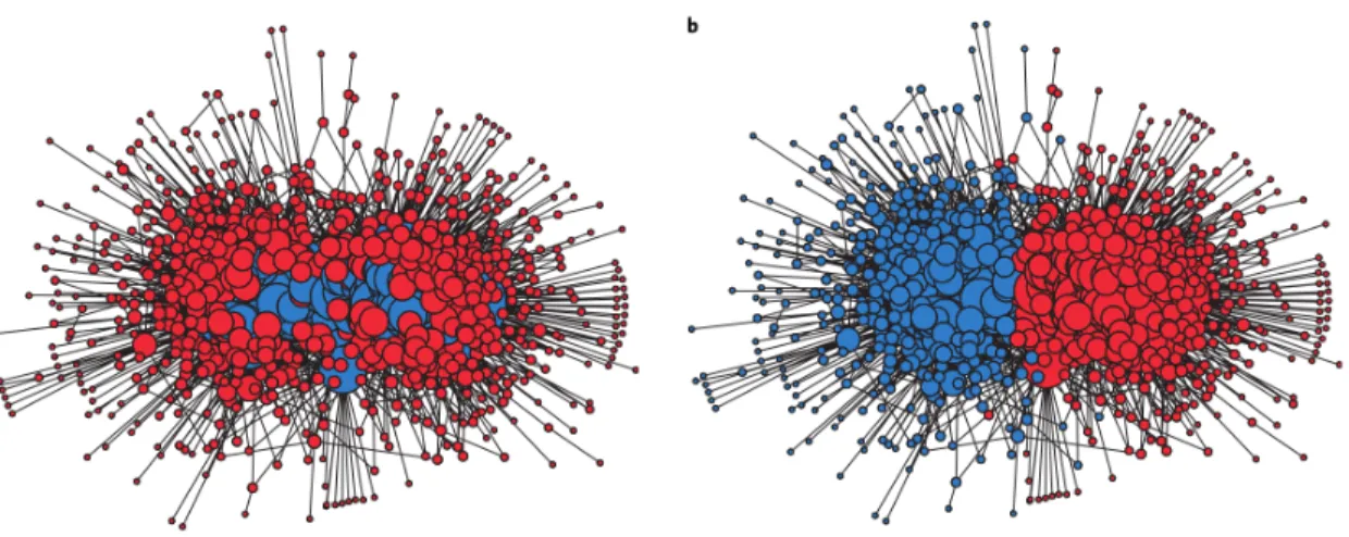
Karrer and Newman (2011) give an excellent example of the usefulness of the DCSBM. In Figure 1.3, we see two community partitions of the same network: one given by fitting the SBM, the other by fitting the DCSBM. The images in Figure 1.3 appear in Newman (2012) as reproductions of those from Karrer and Newman (2011). The network data comes from internet scraping of links between political blogs (Adamic and Glance, 2005), and is equipped with an acknowledged ground truth which labels each blog as politically “liberal” or “conservative”. The visualization was constructed without knowledge of this ground truth, using only the links between nodes. Nodes are colored by their labeling under the choice of model, and are sized based on their degree. We see that using the Degree-Corrected SBM, the estimated labels correspond to the visualization layout, which means the labeling follows patterns of stronger or weaker edge densities between node subsets. In contrast, using the standard SBM, the estimated labels follow the degree distribution: nodes are split into two groups of larger and smaller degrees. Furthermore, as reported in Karrer and Newman (2011), the estimated labels from the SBM have almost no association with the acknowledged ground truth given in Adamic and Glance (2005), whereas the DCSBM labels closely align with the political division.
Figure 1.3: Visualization of a political blog network, labels estimated by the standard SBM (a) and the DCSBM (b) (Newman, 2012).
1.3.3 Consistency of community detection methods
An important, general issue about community detection is the consideration of any given method’s ability to recover “true” communities in the network. In the community detection liter-ature, this issue is framed as consistency under an appropriate generative model. The generative model is almost always taken to be the SBM or some variant thereof. The definition of consistency varies depending on the method under study and the constraints of the theoretical analysis, but it is most often a high probability statement about the clustering error as the number of nodes
n tends to infinity. This sub-section contains a thorough review of some prominent consistency analyses of community detection methods.
Early work on consistency of community detection largely focused on simple versions of the SBM, restricting the number of blocks to 2 (Snijders and Nowicki, 1997), or forcing community sizes and connection probabilities to be equivalent (Condon and Karp, 2001). These analyses will not be discussed in detail, since modern-day consistency analyses have largely eliminated these assumptions. For instance, Bickel and Chen (2009) proved the consistency of the modularity and SBM likelihood partition measures under the SBM with an arbitrary number of blocks. Their analysis begins in consideration of the maximizer ˆcnof a general partition measure (like modularity). The maximizer ˆcn is assumed to be estimated from a n-node SBM with a fixed number of blocks
Bickel and Chen (2009) defined consistency of a partition measure by
Pn(ˆc=c)→1 asn→ ∞, (1.6)
where the partition vector equivalence is defined up to permutation of the community labels. They show that a general class of partition measures which includes modularity and the SBM likelihood are consistent in the above sense. Their result depends on a few key assumptions:
• The average degree of the SBM grows faster than logn.
• The true model partition maximizes the limiting partition measure. • The relative community sizes are positive and do not change withn.
• The matrix Phas entries of the same asymptotic order and unique columns.
Along with a few other technical conditions on the partition measure, these assumptions are a significant improvement over those found in preceding consistency analyses of community detection and graph partitioning algorithms. Zhao et al. (2012) generalized the analysis of Bickel and Chen in the following important ways:
1. Instead of taking the standard SBM as the generative model, they assumed the Degree-Corrected SBM (see Section 1.3.2).
2. They defined a notion of in-probability (“weak”) consistency, as follows: The maximizer ˆcn is weakly consistent if for any >0,
Pn
n−1 X
u∈[n]
1{ˆcn(u)6=cn(u)}<
→1 asn→ ∞. (1.7)
Above, the partition equivalence is again defined up to a permutation of labels. They showed that, under assumptions similar to those from Bickel and Chen (2009), maximzers ˆcn are weakly consistent if the average degree tends to infinity. They also proved the strong consis-tency analog to Bickel and Chen (2009), in the sense of (1.6), when the average degree must grow more quickly than logn.
The work of Bickel and Chen (2009) and Zhao et al. (2012), described above, have been crucial to understanding the properties and performance of partition measures on networks with commu-nities. However, it important to note that their results pertain only to the global maximizer of any given partition measure, which in almost all practical situations is computationally prohibitive to produce. This is a non-trivial problem, since local optimizers of partition measures often have diverse community structures (Peel et al., 2016). The consistency of local optimizers has received comparatively little attention, since a local optimizer is algorithm-dependent. Consistency results for common variational algorithms used to fit the SBM have been given by Choi et al. (2012) and Celisse et al. (2012), among others. However, these results generally require stronger assumptions on the sparsity of the network.
Another important class of consistency analyses for community detection focuses on spectral methods. Lei et al. (2015) prove that, under assumptions as weak as, if not weaker than, those in the aforementioned optimization-based analyses, the asymptotic clustering error obtained in practice by spectral methods is bounded by a function of the average degree, number of communities, ratio of the maximum and minimum community sizes, and the ratio of the maximum and minimum connection probabilities. This is a general result that contains some of the weakest assumptions available for spectral community detection methods. However, spectral methods are in general more computationally prohibitive than modularity maximization, especially for very large networks. Though the analysis of spectral methods for community detection is a vast field with many open problems, the field will not be discussed in any more depth here, since the consistency analyses in this thesis are more closely related to those for modularity and the SBM likelihood.
1.3.4 Community detection for multilayer and bipartite networks
studying individuals with multiple sociometric relations (Fienberg et al., 1980, 1985), and analyzing relationships between social interactions and economic exchange (Ferriani et al., 2013). Kivel¨a et al. (2014) and Boccaletti et al. (2014) provide two recent reviews of the study of multilayer networks. The development of community detection methods for multilayer networks is still relatively new. One common approach to multilayer community detection is to project the multilayer net-work in some fashion onto a single-layer netnet-work and then identify communities in the single layer network (Berlingerio et al., 2011; Rocklin and Pinar, 2013). A second common approach to multi-layer community detection is to apply a standard detection method to each multi-layer of the observed network separately (Barigozzi et al., 2011; Berlingerio et al., 2013). However, the first approach fails to account for layer-specific community structure and may give an oversimplified or incom-plete summary of the community structure of the multilayer network; the second approach does not enable one to leverage or identify common structure between layers. Methods introduced in this thesis will avoid some of these limitations.
In addition to the methods above, there have also been several generalizations of single-layer methods to multilayer networks. For example, Holland et al. (1983) and Paul and Chen (2015) introduce multilayer generalizations of the stochastic block model from Wang and Wong (1987) and Snijders and Nowicki (1997). Peixoto (2015) considers a multilayer generalization of the stochas-tic block model for weighted networks that models hierarchical community structure as well as the degree distribution of an observed network. Paul and Chen (2016) describe a class of null models for multilayer community detection based on the configuration and expected degree model. Stanley et al. (2016) considered the clustering of layers of multilayer networks based on recurring community structure throughout the network. Mucha et al. (2010) first extended the notion of modularity to multilayer networks, and De Domenico et al. (2015) generalized the map equation, which measures the description length of a random walk on a partition of vertices, to multilayer networks. De Domenico et al. (2013) discuss a generalization of the multilayer method from Mucha et al. (2010) using tensor decompositions.
1.3.4.1 Bi-partite networks
Another type of network is known as a “bipartite”. Bipartite networks have two defining properties. First, the node set [n] is bisected into two non-overlapping node setsN1 andN2 of sizes
n1:=|N1|and n2 :=|N2|. Second, edges pair nodes only when one node is fromN1 and the other is fromN2. In other words, if two nodes are from the same side of the network, no edge can exist to pair them.
Note that the division of the node set in bipartite networks is of a different character than the division of an edge set into multiple layers, as in the multi-layer setting discussed in the preceding part of this section. Whereas a multi-layer network has multiple edge sets corresponding to a unified node set, a bipartite network has multiple (two)node sets with a shared edge set.
Formally, a bipartite network can be written as G= (N1, N2, A), whereN1 and N2 are disjoint node sets, and the adjacency matrixA is an|N1| × |N2|matrix containing edge indicators between for edges between nodes in N1 and nodes in N2. Communities in bipartite networks are in fact bi-communities. A bi-community (C1, C2)∈2N1 ×2N2 consists of a node set from each side of the network. In applications, it is of interest to find bi-communities (C1, C2) such that nodes inC1 are strongly connected to nodes in C2, but weakly connected to other nodes inN2, and vice-versa.
Some community detection methods for bipartite networks have been published and well-cited (e.g. Barber (2007); Du et al. (2008); Liu and Murata (2010)). More recently, Bartlett (2015) extended spectral community detection to bipartite networks. One growing area of application of bipartite community detection is when the node sets are genomic markers, and edges indicate a certain level of interaction strength or statistical correlation (e.g. Platig et al. (2015)).
1.4 Contributions of this thesis
The specific contributions in this thesis follow two broad directions, listed below. Note that notations not defined in Section 1.1 are used loosely, will be defined explicitly in the corresponding chapters.
1. Adapt testing-based extraction to general networks data. The testing-based ex-traction algorithm ESSC, mentioned in Section 1.3.1, was limited to binary, single-layer, undirected networks. In my work, I formalize the testing-based extraction approach in a way generalizable to almost all types of network data. Suppose we are given a networkG= ([n],D) withD∈ D. Two components are needed to perform testing-based community extraction:
• A null modelPθ onDwhich specifies a notion of “lack of association” for arbitrary nodes and sets u andB.
Chapter 2 is devoted to a rigorous treatment of these concepts. In practice, the testing framework components T and Pθ are not always easy to formulate, since D can consist of data of many different types. Multiple projects in this thesis involve an adaptation of testing-based extraction to new types of network data.
2. Assess the statistical consistency properties of extraction methods. The consistency properties of extraction methods have not yet well-investigated. In this thesis, new concep-tions of consistency for extraction algorithms are introduced, and consistency properties of proposed methods under various models with planted communities are established.
The following sections introduce specific contributions of this thesis with respect to the direc-tions above.
1.4.1 Community extraction for edge-weighted networks
Recall from Section 1.2 that many classical community detection methods are based, in some way, on a null model. A significant drawback of these methods is that no explicit null model exists for edge-weighted networks. Edge weights are commonplace in network data, and can provide infor-mation that improves community detection power and specificity (Newman, 2004a; Boccaletti et al., 2006). While many existing community detection methods have been established for weighted and un-weighted networks alike, due to the absence of an appropriate weighted-network null model, very few of these methods provide statistical significance assessments of weighted-network communities. In contrast, some significance-based community detection methods have recently been introduced in the literature forun-weighted networks, due to the popularity and acceptance of the configura-tion model as a binary-network null. These methods, OSLOM from Lancichinetti et al. (2011) and ESSC from Wilson et al. (2014), were discussed in some detail in Section 1.3.1. While OSLOM can in practice handle edge weights, the method uses an exponential function to calculate nominal tail probabilities for edge weight sums, a testing approach which is not based on an explicit null. As a consequence, communities in weighted networks identified by this approach may in some cases be spurious or unreliable, especially when no “true” communities exist.
The project presented in Chapter 3 has a three-fold purpose: (i) to provide an explicit null model for networks with weighted edges, (ii) to present a community extraction method based on hypothesis tests with the null, and (iii) to provide an analysis of the consistency properties of the method with respect to a weighted stochastic block model. These contributions provide steps toward a rigorous statistical framework with which to study communities in weighted networks. Results of extensive simulations show that the proposed extraction method is more successful than competitors at identifying overlapping and background nodes. The method also extracts communities that align with key features of real data.
1.4.2 Community extraction for multi-layer, binary networks
As discussed in Section 1.3.4, some approaches to multi-layer networks proceed by either ag-gregating layers into a single-layer weighted or multi-edge network, or by assuming that the same community structure exists across all layers. In general, these practices ignore potential layer-wise heterogeneity. As just one example from social networks, a group of individuals may be well-connected via friendships on Facebook; however, this common group of actors will likely, for example, not work at the same company. In realistic situations such as these, a given vertex community may only be present in a proper subset of the layers. It may be of practical interest to determine the persistence properties of such a community across various layer sets, something which layer-aggregation or homogeneous multi-layer modeling cannot accomplish. In general, com-plex and differential relationships between actors will be reflected in heterogeneous behavior of different layers, behavior which existing multi-layer network community detection methods, for the most part, cannot capture.
1.4.3 eQTL analyses and bi-partite correlation networks
In Chapter 5, new methods to study expression Quantitative-Trait Loci (eQTL) networks are presented. An expression Quantitative Trait Locus (eQTL) is a genetic polymorphism (typically a single-nucleotide polymorphism, abbreviated by SNP) that is associated with transcriptional ex-pression levels in a particular tissue. The statistical analysis of eQTLs has become increasingly important in understanding molecular mechanisms by which genetic variation gives rise to complex traits and human disease (cf. Morley et al. (2004); Gilad et al. (2008); Grundberg et al. (2012); Westra et al. (2013)). For example, eQTL studies can be used to plausibly link disease pheno-types analyzed in Genome-Wide Association Studies (GWAS) to gene expression, with recent work focusing on variation across tissues (Gamazon et al., 2015; Ardlie et al., 2015). Although the un-derlying biology is complex, a fundamental step in many analyses is to compare the genotypes of a large number of SNPs to the expression levels of all known genes, which presents challenges in computation and multiple testing (Wright et al., 2012). Effectively, the quantitative results of these comparisons are edge weights on a complete bi-partite network consisting of SNP loci (henceforth just called “SNPs”), on one side, and genes, on the other.
The first section of Chapter 5 presents a new model for investigating the association strength of asingle gene-SNP pair. Statistical analyses of eQTLs have often been based on standard linear regression (Shabalin, 2012), with a focus on testing and detection of gene-SNP pair relationships. A key step, commonly considered necessary to avoid false positives, has been to normalize and transform the expression data prior to analysis (Beasley et al., 2009). However, normalization removes the scale of the expression data, and with it, a natural measure of effect size due to genotype. As a consequence, eQTL effect size has often been described in terms of regression partial R2 between genotype and transformed expression (see for example Stranger et al. (2007)). However, theR2 statistic can be highly sensitive to transformations of the response, and is difficult to interpret biologically. An appropriate eQTL model should reflect a coherent model of allelic contributions to expression, and be able to capture and describe evidence of dominance that is still rarely examined in detail (Powell et al., 2013). Furthermore, a biologically appropriate effect-size model improves the accuracy of hypothesis tests (as I will show), and provides reliable rankings of eQTLs in terms of effect sizes as opposed to p-values.
In Section 5.1, I propose ACME-eQTL, a new model for the effect size of cis-acting eQTLs, in which the effects of allele count on expression are Additive Contributions on the original expression scale, with Multiplicative Error. In the ACME-eQTL model the log of expression is equal to the log of a linear systematic term (“log-of-linear”) plus noise and covariate effects: this subtle difference from standard log-linear modeling is of key importance in estimating and interpreting effect sizes. Although the ACME-eQTL model is straightforward, it reflects a marked departure from standard practice in eQTL analyses and has important implications for inferences from effect sizes. The major contributions of this project are efforts to: (i) motivate and introduce the model, (ii) provide a novel fitting algorithm and corresponding software package, and (iii) derive a means to calculate and evaluate appropriate p-values. To support the use of the model, goodness-of-fit tests are performed on real data from the GTEx Project (Lonsdale et al., 2013). Also considered are the model’s robustness to skew in the residuals (under the null), and its superior power and estimation accuracy compared with existing models (under the alternative).
In Section 5.2, the second section of Chapter 5, I introduce preliminary work on a community detection method for eQTL networks. Rather than analyzing individual gene-SNP pairs, this method assesses groups of eQTLs in the search for mutually cross-correlated sets of genes and SNPs. This methodological research direction is relatively new, and has been applied to eQTL networks in a few recent publications, for example in Huang et al. (2009); Bao et al. (2010); Platig et al. (2015). The trend in these publications (among others) is to use the following general procedure:
1. Compute all cross-correlations between genes and SNPs.
2. Dichotomize the cross-correlations through some inferential procedure.
3. Perform a binary community detection routine on the resulting bi-partite network.
vary widely, so any threshold will be necessarily insufficient to capture the complex relationships in the network. Furthermore, some community detection methods for bi-partite networks are based on null models (e.g. Barber (2007)) that carry assumptions unreasonable for binary networks formed by discretized correlations. In particular, a dichotomized correlation network contains edge-to-edge correlations determined by the underlying partial-correlation structure of the expression data, correlations which are not accounted for in standard models for binary graphs.
The community detection method for bi-partite correlation networks that I introduce, called “Correlation Bi-Community Extraction” (CBCE), overcomes both of the aforementioned issues. CBCE is formulated through a bi-partite network adaptation of the testing-based extraction frame-work. In this setting, which is described in full in Section 5.2, the goal is to recover eQTL bi-communities, consisting of a gene-subset, SNP-subset pair with large observed cross-correlations. Being an extraction method, CBCE searches for modules one-by-one, which eliminates the need to compute all cross-correlations or a full binary bi-partite network. This greatly reduces the com-putational burden of the aforementioned approach. Furthermore, the hypothesis testing inherent to CBCE is able to deal with the observed correlations directly, employing a specific null model for correlation sums. In other words, CBCE directly uses all information available in the raw correlation data, and is based upon a principled null model that reflects the correct distribution of the variables at play. In Section 5.2, I detail the CBCE algorithm in full, provide theoretical support for a p-value approximation, and show preliminary results comparing its performance to some existing methods on simulated data.
1.5 Document Organization
The rest of the document is organized as follows. In Chapter 2, I present the testing-based extraction framework in generality. In Chapters 3-5 that follow, I present the full scope of my work on the projects introduced in Sections 1.4.1-1.4.3 (respectively).
CHAPTER 2
Node-Set Testing for Complex Networks
Though community detection methods vary widely, the notion of a “community” usually in-volves the characteristic that constituent nodes are strongly internally associated, but weakly ex-ternally associated. As discussed in Section 1.2, many classical approaches to detect this type of association in networks rely on a univariate score of a node partition. Dependence on a partition score can be limiting, since such a score must assess the communities defined by the partition simultaneously, with one number. Furthermore, the vast majority of partition-based methods do not come with a natural conception of statistical significance.
In this chapter, a methodological framework called Node-Set Testing (NST) is introduced for community detection on networks with potentially multiple, heterogenous data types. The NST framework involves explicit notions of statistical significance, and is motivated by recent iterative testing-based methods introduced by Lancichinetti et al. (2011) and Wilson et al. (2014). These methods, however, involve significance tests for binary networks only, and do not rigorously establish the theoretical underpinnings of the approach. NST introduces a general yet rigorous definition of a community that does not depend on any partition score. A generalized community extraction algorithm for networks is then built around this definition. A theoretical result is established regarding the error properties of the proposed extraction method.
2.1 Node-Set Testing Framework
when weights can be zero despite the existence of an edge. In general, a full network data object can be denoted by the double G:= ([n],D).
Define an association function a : [n]×2[n] 7→ R as some measure of the true relationship between nodes and sets in G. For any u ∈ [n] and B ⊆ [n], a(u, B) > 0 indicates positive association betweenuand B,a(u, B)<0 indicates negative association, anda(u, B) = 0 indicates no association. Usinga(u, B), the notion of a community can be formally defined, as follows:
Definition 1. Given a: [n]×2[n]7→R, a community is any node set C⊆[n]satisfying (i) a(u, C) is positive for eachu∈C, and
(ii) a(u, C) is non-positive for everyu∈Cc.
The function a is a stand-out feature of the NST approach to community detection. In most community detection methods, the meaning of “association” is tied to a fixed objective function (like modularity or within-sum-of-squares). In contrast, in the NST framework, we have complete freedom in our notion of association, and thus also in our notion of a community. Most often, a
will have an interpretation as a “ground-truth” or “population” value of some empirical measure of association. Thus, strictly speaking,a(u, B) will depend on some (unknown) distributionPthat is assumed to have generated the data D. Here are examples of association functions from two different types of networks:
1. Let G = ([n], A) be an undirected binary network with distribution P. Define the expected edge count betweenu and B underP by
¯
d(u, B) :=E
X
v∈B
A[u, v]
!
. (2.1)
As discussed in Section 1.2.2, the appropriate null for binary networks is the Chung-Lu (or configuration) model, in which edge probabilities are proportional to expected degrees. Therefore, for us to call u and B truly associated, ¯d(u, B) should be greater than the sum of the corresponding null edge probabilities. Explicitly, let ¯d(u) be the expected degree of
u under P, and ¯dT the sum of expected degrees (as in Section 1.1). Recall that, if P is the Chung-Lu model, we have P(A[u, v] = 1) = ¯d(u) ¯d(v)/d¯T. Thus, an appropriate association
function is
a(u, B) := ¯d(u, B)−X v∈B
¯
d(u) ¯d(v) ¯
dT
:= ¯d(u, B)−d¯(u)¯q(B), (2.2)
with ¯q(B) := ¯d−T1P
v∈Bd¯(v), the expected relative edge-density of B under the null. The value ¯q(B) is essentially the null probability that a randomly chosen edge connects to a node in B. Thus, an interpretation of (2.2) is that u and B are associated if and only if ¯d(u, B) exceeds the null-expected proportion ofd(u) incident withB.
2. Let X∈Rd×n be a matrix of Euclidean data. Define a correlation network by G = ([n],X), where edges are identified with the sample Pearson correlations of thed-dimensionalX data. AssumeXhas populationn×ncorrelation matrix Σ, with general elementρ(u, v). Then the natural association function for detecting communities with high average internal correlation is
a(u, B) := X v∈B
ρ(u, v). (2.3)
Unlike in the previous example, the sum of the edge population valuesρ(u, v) is the association measure of interest, and is equal to zero under the null, without centering. This contrast shows the flexibility of the NST approach across different types of networks.
In the next section, a statistical approach to significance tests for values of a(u, B) is laid out, yielding a general NST community extraction algorithm.
2.2 Node-set association testing
Let D represent the product space of the data D = (D1, . . . , Dm). To discover communities satisfying Definition 1, we assume the existence of a summary statistic T : [n]×2[n]× D 7→ R with the characteristic that large enough values of T(u, B,D) suggest positive values of a(u, B). We also assume the existence of an explicit null model Pθ which gives the distribution of D ∈ D when a(u, B) = 0. Here,θis a parameter (or set of parameters) for the null model. Assumingθ is known, we can test the hypotheses
with the one-sided p-value
p(u, B,D) :=Pθ T(u, B,De) > T(u, B,D)
, (2.5)
where De is a random realization of the network data under the null. However, in practice θ is
rarely known. Usually, θ must be estimated or set to plug-in values computed from the data. This is analogous to the treatment of the unknown parameterp in a standardz-test of a binomial random variable. The canonical confidence interval forp depends onp itself. Thus, the maximum likelihood estimate ˆpis used in the formula for the interval, even though ˆp is also the test statistic of interest. Data-dependent measures of connection strength are also not without precedent in community detection methodology. In the modularity score, for instance, empirical degrees are stand-ins for the (unknown) expected degrees of the Chung-Lu/configuration model.
Illustrating choices ofT andPθ in practical situations, the examples laid out in Section 2.1 are continued:
1. To complete the NST framework for binary undirected networks, first recall that in this setting, the network data is simplyD=A, the adjacency matrix. We continue to writeDto conform to generic notation. In this setting, we use the test statistic
T(u, B,D) := X v∈B
A[u, v], (2.6)
and the Chung-Lu null model with parameter θ = ( ¯d(1), . . . ,d¯(n)). In practice, θ is set to the empirical degrees (d(1), . . . , d(n)). LetEdenote expectation underP, the true generating model ofD. LetEθ denote expectation underPθ. Then
a(u, B) := ¯d(u, B)−d¯(u)¯q(B) =E
T(u, B,D)
−Eθ
T(u, B,De)
Hence, ifa(u, B) is positive, the p-value in (2.5) will be stochastically larger than uniform.
2. Finishing the NST framework for correlation networks, we recall thatD=X, the Euclidean data for the nodes [d], and define the test statistic
T(u, B,D) :=X v∈B
r(u, v), (2.7)
wherer(u, v) is the Pearson correlation between nodeuandv. Regarding the null model, re-call thatXis assumed to have true population correlations Σ with general entryρ(u, v). Under the null corresponding to the hypotheses (2.4), we assume thata(u, B) :=P
v∈Bρ(u, v) = 0. If in fact a(u, B) is positive, however, the p-value in (2.5) will be stochastically larger than uniform. Note that the distribution ofT(u, B,De) depends on Σ. Therefore, we calculate the
p-value in (2.5) with the parameter θ= ˆΣ, the estimated correlation matrix ofX.
Derivations of closed-form expressions for the p-values in the examples above are part of their respective applications of NST, and outside the scope of this framework. Wilson et al. (2014) provided an asymptotic result for (2.6), which facilitated an approximate p-value in that setting. Bodwin et al. (2015) gave a central limit theorem for a test-statistic similar to (2.7) for the mining of differential correlation. Similar theoretical results are major components of my work on the NST methods, introduced in the subsequent chapters of this thesis.
2.3 The Stable Community Search (SCS) algorithm