RAPID ENROLLMENT DESIGN FOR FINDING THE OPTIMAL DOSE IN IMMUNOTHERAPY TRIALS WITH ORDERED GROUPS AND OPTIMAL DESIGN
OF EXPERIMENTS WITH OBSERVATION CENSORING DRIVEN BY RANDOM ENROLLMENT
Xiaoqiang Xue
A dissertation submitted to the faculty at the University of North Carolina at Chapel Hill in partial fulllment of the requirements for the degree of Doctor of Public Health in the
Department of Biostatistics in the Gillings School of Global Public Health.
Chapel Hill 2019
Approved by: Anastasia Ivanova Valerii V. Fedorov Jason Fine
ABSTRACT
Xiaoqiang Xue: Rapid enrollment design for nding the optimal dose in immunotherapy trials with ordered groups and optimal design of experiments with observation censoring
driven by random enrollment
(Under the direction of Anastasia Ivanova and Valerii V. Fedorov)
In addition to variability between subjects in clinical trials we face uncertainty caused by enrollment process. Due to uncertainty in enrollment, the follow-up times are random, which makes the amount of information gained during experimentation random as well. This is especially a concern for clinical trials with time-to-event endpoints where the event time and censoring time are impacted by a random enrollment process. We have developed an optimal design theory for clinical trials with time-to-event endpoint and random enroll-ment. To account for uncertainty caused by the enrollment process, we consider the aver-age elemental information matrix and develop methods based on maximizing the averaver-age information or to guarantee that the information is greater than a pre-specied value with a given probability. We illustrate the approach using proportional hazard models with cen-sored observations and enrollment that follows the Poisson process.
To Decheng Xue and Lufen Wang, my parents who give me unconditional love and support. To Dongxia Li, my wife for all supports.
To Ryan Xue, Brady Xue, and Charlotte Xue, my sweet kids for all the enjoyment and pleasure.
ACKNOWLEDGMENTS
I would like to express special thinks and deep gratitude to my inspirational advisors, Dr. Anastasia Ivanova and Dr. Valerii V. Fedorov, for continuous support and encourage-ment, for their patience for my struggles, and for their generosity with their time. I would also like to acknowledge my committee, Dr. Jason Fine, Dr. Matthew C. Foster, and Dr. Xianming Tan, for their patience and insight into my research.
I would also like to thank IQVIA, where I have worked for many years of this doctoral program. IQVIA provided nancial support to me over the doctoral program years. In ad-dition, IQVIA allowed for exible work schedules when needed in order to pursue academic interests.
I could not express my gratitude to my parents, brother and sisters, especially my youngest sister who sacriced her dream to support me when we were young. My parents, who
never had chance to nish their elementary schools, inspire me everyday with their hard working ethic.
Last but not the least, my wife, Dongxia Li, and my three lovely children, Ryan, Brady, and Charlotte, for all unconditional support, and joyfulness in the past several years. With-out them, all of this would be meaningless.
TABLE OF CONTENTS
LIST OF TABLES ... ix
LIST OF FIGURES ... x
CHAPTER 1: LITERATURE REVIEW ... 1
1.1 Literature... 1
1.1.1 Introduction for optimal design for survival clinical trials ... 1
1.1.2 Introduction for dose nding studies ... 7
CHAPTER 2: SURVIVAL MODELS WITH CENSORING DRIVEN BY RANDOM ENROLLMENT ... 13
2.1 Introduction ... 13
2.2 Model ... 14
2.2.1 Elemental information matrix in survival anal-ysis setting ... 16
2.3 Random subject accrual... 17
2.4 Example: proportional hazard family ... 21
2.5 Conclusion... 22
CHAPTER 3: OPTIMAL DESIGN OF EXPERIMENTS WITH THE OBSERVATION CENSORING DRIVEN BY RAN-DOM ENROLMENT OF SUBJECTS ... 23
3.1 Introduction ... 23
3.1.1 Elemental information matrices ... 25
3.1.3 Elemental information matrix in survival
anal-ysis setting ... 27
3.2 Optimal design for non-staggering entry ... 30
3.3 Random subject accrual... 32
3.4 Properties and numerical procedures ... 37
3.4.1 Properties of locally optimal designs ... 37
3.4.2 Numerical procedures ... 38
3.5 Example ... 40
3.6 Conclusion... 41
CHAPTER 4: RAPID ENROLLMENT DESIGN FOR FIND-ING THE OPTIMAL DOSE IN IMMUNOTHERAPY TRI-ALS WITH ORDERED GROUPS ... 43
4.1 Introduction ... 43
4.2 Estimating under order restrictions ... 46
4.2.1 Notation ... 46
4.2.2 Isotonic estimation of toxicity and response probabilities in a trial with ordered groups ... 46
4.3 Examples ... 48
4.4 The rapid enrollment design to nd the optimal doses in two ordered groups ... 49
4.5 Migrating for delayed toxicity and clinical response... 52
4.6 Simulation study ... 53
4.7 Conclusions... 57
LIST OF TABLES
3.1 Elemental Information matrices ν(η, T) for the most popular distribution with τ ∈ {0, T} and censoring
time T ... 29 3.2 The expected elemental information matricesν(Te, Ts, η)
for the dierent distribution of censoring time Tf =
Ts−t, for exponential distributed lifetime... 36 3.3 Sensitivity functions ψ(x, ξ), D=M−1 ... 38 4.4 An example of Bayesian isotonic estimation in a single
group. Observed counts are presented as the number
of outcomes over the total number of patients at the dose ... 49 4.5 An example of Bayesian isotonic estimation under
constrains in (1) in two groups. Observed counts are presented as the number of outcomes over the total
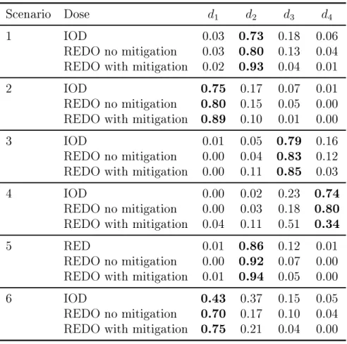
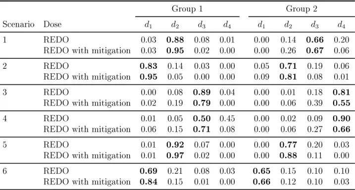
number of patients at the dose ... 50 4.6 Scenarios with four doses and two ordered groups ... 55 4.7 Comparison of the design to nd the optimal dose
from Ivanova (2003) (IOD) and the REDO. The rec-ommended optimal dose in a single group trials for group 1 in scenarios in Table 4.6. The true optimal
dose is shown in bold ... 56 4.8 Proportion of trials each dose was recommended as
the optimal doses in two ordered groups trials for sce-narios in Table 4.6. The true optimal dose is shown
LIST OF FIGURES
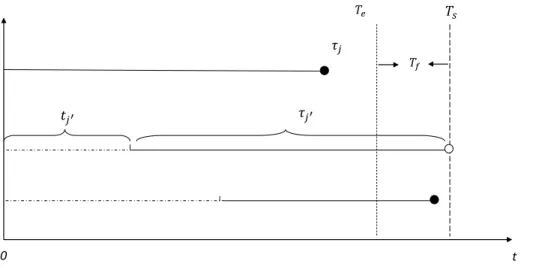
1.1 Staggered entry,tj stands for arrival time,τj exposure time; enrollment starts att = 0and stops att=Te; ◦
indicates censoring;•indicates an event; a trial stops
CHAPTER 1: LITERATURE REVIEW
1.1 Literature
1.1.1 Introduction for optimal design for survival clinical trials
In a clinical trial where the association between study treatment and time to the treatment-related event is the primary interest, study units do not always experience endpoint event, because either the experiment was terminated before endpoint event is observed or study individual was lost to follow-up, in which case study unit was censored.
Methods for survival analysis could be tracked back to several hundred years ago when the life table was proposed by Halley (1693). Kaplan and Meier published a manuscript the statistical properties of a non-parametric method for incomplete data in 1958, although Partial likelihood method proposed by Cox (1972) introduced regression techniques into survival analysis. One of the important assumptions that Cox regression requires is the proportional hazards assumption, which does not always hold. In the situation where the proportional hazard is not realistic, stratied Cox model Kalbeisch and Prentice (1980) or Cox regression with time-varying covariates Kalbeisch and McInocsh (1977) are fre-quently employed. Another method to use when the assumption of constant hazard is not satised, is the accelerated failure time (AFT) model Wei (1992), which models the eect of an explanatory variable on the survival time rather than hazard. The AFT has been mainly a part of statistical method for manufacturing.
nd a copy of a statistical journal without articles in survival analysis. However, research in survival analysis has primarily been focusing on parameter estimation by modeling life-time McGree and Eccleston (2009) while the design of life-time-to-event experiments has not draw much attention until recently, and we will provide a survey on this development in the following texts.
which could be expanded to more levels for discrete space or continuous space. Expand-ing from full likelihood based on exponential distribution, a locally optimal experimen-tal design for Cox proportional hazard model with partial likelihood was considered by Lopez-Fidalgo and Rivas-Lopez (2012). In this development, all patients were assumed to enroll in a trial at the same time which is less practical, and two distinct types of cen-soring are considered, dropout before study complete at d and right censoring at time d. The Fisher information matrix was developed based on the partial likelihood in general with pdf h(t|x) = h0(t|x) exp{θ>x} whereh0(t|x)is the baseline hazard function and θ is m− dimension regression parameters to be studied, the exponential distribution for both
censoring, where censoring moment c= inf, and it becomes an optimal design for general-ized linear model. The D-optimal design with link function λθ(s) = exp(θ0 +θ1s)is found to be two-point design when θ1 ≤ kS2
u e k−1
on design region (0, Su] wherek =cexp(θ0) (see details in Muller, 2013). The optimal designs considered above Lopez-Fidalgo et al. (2009), Lopez-Fidalgo and Rivas-Lopez (2012), Konstantinou et al. (2011), Muller (2013) are some special case with special assumptions about the time to events, time to dropout and time to subject arrivals.
Atkinson et al. (2012) and Fedorov and Leonov (2014) recommended generalization of optimal design for generalized linear model for the cases where Fisher information and regular maximum likelihood estimators exist, following well organized steps:
1. Dene a model Y ∼ p(y|η), for the response variable, η = η(x, θ)where θ>(x, θ) =
{η1(x, θ),· · · , ηk(x, θ)} are given functions of controlsx ∈ X and unknown regres-sion parameters θ;
2. Calculate the elemental information matrix ν(η) = Varh ∂
∂ηlnp(y|η)
i
, and con-struct information matrix for single observation Atkinson et al. (2012), µ(x, θ) = F(x, θ)ν(η)F>(x, θ), where F(x, θ) = ∂η>∂θ(x,θ). Total information matrix M(θ,{xi}n1) =
Pn
i=1µ(xi, θ). Elemental information matrix for most popular univariate distribution and bivariate distribution are available in Atkinson et al. (2012) and Fedorov and Leonov (2014).
3. Dene the design region x∼X and controls ξ ={wi, xi}n1;
4. Following the paradigm of convex design theory Fedorov (1972), Fedorov and Leonov (2014), and dene the optimal design as ξ? = arg min
and Leonov (2014), necessary and sucient condition for ξ? to be optimal is fulll-ment of the inequality minx∈X ψ(x, θ) ≥ 0, whereψ(x, θ) is called the sensitivity
function, and most population criteria can be found in Atkinson et al. (2012) and Fedorov and Leonov, (2014). Numerical procedures can be developed following this equivalence theorem to search for the optimal design.
In this development, we will follow these well developed steps Atkinson et al. (2012) and Fedorov and Leonov (2014) recommended.
Compared to a xed design, where typically all participants are followed up for T years in the study, the clinical trial studying the “time to event” data typically is terminated at a common date for all subjects, when a pre-dened Sth event is observed to power the study. As described by Fridman et al. (2010), some subjects experience the event in the scheduled follow-up period, while others will be censored during follow-up. In Figure 1.1, with four subjects experiencing events before study is completed, two subjects are cen-sored at study close, and two subjects are cencen-sored before the study completed, due to other reason, for instance, lost-to-follow up, or competitive events. In survival analysis, the data likelihood function and the information matrix can be computed based on the failure time and censoring mechanism after the data were collected, however, neither the case of censoring nor the censoring time is known before the study being conducted.
𝑡𝑗′
𝑇𝑠
𝜏𝑗′
0
𝑇𝑒
𝑇𝑓
𝜏𝑗
t
Figure 1.1: Staggered entry, tj stands for arrival time, τj exposure time; enrollment starts att = 0 and stops at t = Te; ◦ indicates censoring; • indicates an event; a trial stops at
t=Ts; Tf is a minimal follow-up period.
Elemental information matrix Fedorov and Leonov (2014) plays an central role in both design and analysis of experiments. The elemental information matrices for most parametric distributions can be found in Fedorov and Leonov (2014). We focus on the ele-mental information matrices for survival data with random censoring. The Fisher informa-tion matrix for Weibull and generalized exponential distribuinforma-tion has been studied for type I censored survival data by Gertsbakh and Kagan (1999) Fisher information matrix for the hazard function and time to event data without censoring has been studied by Efron and Johnstone (1990). Extensive work for Fisher information under Type II censoring has been done under Weibull family Zheng (2001).
In what follows, dierent censoring distributions, such as uniform distribution, Gamma distribution, truncated Gamma distribution, and Beta distribution will be applied with exponential and Weibull distributions for time to event.
(1989). (3) to illustrate the proposed design and compare various designs via simulations with numerical iterative algorithm.
1.1.2 Introduction for dose nding studies
Drug development in oncology is dierent from most other therapeutic areas, as ac-tual patients are enrolled in phase I oncology studies while health volunteers are typically recruited for others. Consequently, toxicity and adverse events are more acceptable for in-vestigators and patients. The main objective of a dose-nding clinical trial in oncology is to estimate the maximum tolerated dose (MTD), which is typically dened as the dose with a certain probability of dose limiting toxicity (DLT) usually in the 20−25% target range. Given the possibility of observing severe adverse events associated with new anti-cancer therapies, escalation to higher doses in dose-nding trials usually occurs gradually. We also would like to minimize the number of subjects assigned to low doses as they might not oer ecacy benets. The anti-cancer activity of a study drug is further evaluated in phase II studies, in which patients receive the dose determined in phase I, which is typi-cally the estimated MTD or a dose right below. Phase II studies are typitypi-cally open-label one arm or multi-arm non-comparative studies.
(2002), Wages et al. (2011), is a more ecient dose-nding method because it utilizes all information collected, not only information at the current dose. In CRM design, a parsi-monious working model is usually used to model the dose-toxicity relationship. The CRM typically assigns more patients in the neighborhood of MTD compared to the 3 + 3 design.
design for dose-nding in phase I/II clinical trials, where bivariate probit model is used as a working model for dose-toxicity and dose-response relationship.
An implicit monotone increasing relationship between dose toxicity and dose level com-monly exists for oncology dose nding studies. Stylianou and Flournoy proposed using isotonic regression estimate for toxicity rate, and showed that this isotonic regression es-timate is superior to other eses-timates in single risk groups of MTD in dose nding studies Stylianou and Flournoy (2002), and the superiority was conrmed in the improved up-and-down designs for phase I trials Ivanova et al. (2003). Ivanova and Wang extended the iso-tonic regression estimate to dose-nding trials with two possibly ordered populations, with possible ordered susceptibility to the study drug Ivanova and Wang (2006). The bivariate isotonic estimator is computed in multiple steps: (1),calculate the proportion of toxicity data at dose dj for both groups, j = 1,2, ...J; (2), set up the order constraints, ψi1 ≤ · · · ≤ ψiJ, i = 1,2 and ψ2j ≤ ψ1j, j = 1,2,· · · , J if the group order is known G2 ≤ G1; (3), Dykstra algorithm Robertson et al. (1988) is employed to compute the bivariate isotonic regression estimator of toxicity rate, by posing the order restrictions in (1),(2) by optimiz-ing the problem P2
i=1
PJ
j=1
ψij −ψˆij
2
= minG2≤G1
P2 i=1 PJ j=1 ˜
ψij −ψˆij
2
≡ M(2,1). When the group order is known to be G1 ≤ G2, replace the constraints (2)ψi1 ≤ · · · ≤ ψiJ, i = 1,2and ψ1j ≤ ψ2j, j = 1,2,· · · , J, and the optimization problem becomes
P2
i=1
PJ
j=1
ψij −ψˆij
2
= minG1≤G2P2i=1PJj=1
˜
ψij−ψˆij
2
≡M(1,2). They recommended to choose the smaller one out of M(1,2), M(2,1) for the estimates when there is no prior in-formation on the group order.
Dunson and Neelon (2003) showed that standard Bayesian approach by assigning 0 prob-ability to region outside of the restraints might lead to biased estimates in small sample samples, and proposed Bayesian isotonic transformation that projects draws from uncon-strained posterior density onto conuncon-strained space using minimal distance mapping. Ivanova et al. (2016) used a Beta-Binomial model for the toxicity probability estimate. Toxicity was dened as a binary outcome of observing a toxicity event within time T from the start of treatment. DLT in phase I oncology trials is typically dened based on 1 cycle of ther-apy that usually lasts3 or 4weeks, while longer periods of time are used for follow-up in radiation therapy trials. For trials with delayed toxicities, several methods have been proposed to use information from all patients not only from patients who completed the follow-up. Cheung and Chappel (2000) considered a time-to-event modication of the CRM. Ivanova et al. (2016) considered a more conservative method to mitigate uncer-tainty in estimated toxicity probability due to patients still in follow-up. A fraction toxi-city of 1−u/T is added to the total toxicity count for each patient still in follow-up, where u is patient's current follow-up time, andT is the full follow-up time.
Since most of oncology drugs are rather toxic, the dose that can be administered to patients is limited by toxicity. A phase 1 study in oncology usually estimates the maxi-mum tolerated dose (MTD) and then therapeutic ecacy of the MTD is evaluated in a subsequent phase 2trial. The MTD is usually dened as a dose with a probability of dose limiting toxicity (DLT) close to target toxicity rateΓ, typically 0.20or0.30. Statistical de-signs for dose-nding methods in oncology has been recently reviewed by Tighiouart et al. (2014) and Sverdlov et al. (2014).
a dose-nding trial is dened based on both toxicity and ecacy. There are a number of ways to dene the target dose based on toxicity and ecacy and a number of methods to estimate such a dose in a dose-nding trial Gooley et al. (1994), Durham et al. (1998), Ivanova et al. (2003). Ivanova (2003) proposed to dene the optimal dose as the dose that maximizes the probability of success, therapeutic response and no toxicity, among doses with the probability of DLT less Γ. Ivanova (2003) described an up-and-down design to estimate the optimal dose.
CHAPTER 2: SURVIVAL MODELS WITH CENSORING DRIVEN BY RANDOM ENROLLMENT
2.1 Introduction
The design of experiments in survival analysis attracted attention from the optimal design of experiments community relatively recently and examples of publications include: Lopez-Fidalgo et al. (2009) considered optimal design for the proportional hazard models, for a two-parameter linear regression model with exponentially distributed survival times and uniformly distributed patient enrollment time, Lopez-Fidalgo and Rivas-Lopez (2012) continued with the proportional hazard model and introduced censoring due to dropout. Other examples include Konstantinou et al. (2011) and Muller (2013). The latter pub-lication contains a survey section that covers most of the developments in this area. All these papers are focused on specic cases and derive the respective equivalence theorems complemented either by numerical procedures or by analytic solutions for relatively simple scenarios.
2.2 Model
Let us start with a diagram of subject arrivals and the respective observations or cen-soring, see Figure 1.1 compare with Chapter 1 Cox and Oakes (1984) or Chapter 10 Frid-man et al. (2010). In this diagram tj stands for the arrival time of the j-th subject, en-rollment stops at Te and follow up continued till Ts (study completion). Each subject j is observed during a time interval τj . We assume that all censoring happen at a t = Ts and thus do not consider censoring related to dropouts either informative or not, cf. Balakrish-nan and Kundu (2013).
Enrollment may be stopped either at the pre-xed time Te = Ts −Tf, whereTf is a xed follow-up period, or at T(ns)when a required number ns of subjects is enrolled, or at a moment T(Rs) when the needed number Rs of events occurred. Various combinations of these stopping rules were discussed in the literature on life-testing experiments, see Bal-akrishnan and Kundu (2013) for a summary of results and further references. In this paper the focus is on the stopping by time case.
We assume that:
Time-to-event is random and its probability density is ϕ(τ, η).
Elemental parameters η depend on variables (controls)x∈X, i.e. η=η(x, θ).
Response functions η(x, θ) are given, nite for all x ∈ X and twice dierentiable
with respect toθ ∈Ω.
Design region X and Ωare compact.
On arrival subjects are randomized across doses {xi}N1 with probabilities{pi}N1 ,
PN
i=1pi = 1.
To identify a subject and related outcomes we will use subscripts ij. At the study com-pletion, the following values become known:
Number of subjects ni assigned to dose xi and all arrival timestij. Note that these values are completely dened by an enrollment process and by the randomization rule.
The outcomes {yij}n1i = {τij, δij}1ni, where δij = 1 if τij ≤ Ts −tij and δij = 0 otherwise.
Most of the distributions that are popular in survival analysis, cf. Cox and Oakes (1984), depend on one or two parameters. The objective of design is to nd dosesx∗i and respec-tive p∗i that minimize a pre-selected function of the variance-covariance matrix of the max-imum likelihood estimator θˆof unknown parameters. The more detailed and more accu-rate denition will be given later. To address the problem we follow the path introduced in Atkinson et al. (2012) and Fedorov and Leonov Chapter 2 (2014) with some additions that take into account censoring and randomness of the arrival times. To do this we are to dene and nd the analogue of the elemental information matrix that is essential for the approach.
In what follows we use the following notation, typical for the analysis of survival data:
Distribution function: Φ(τ, η) = ´0τϕ(t, η)dt.
Survival function: S(τ, η) = 1−Φ(τ, η).
Hazard function: h(τ, η) = ϕ(τ, η)/S(τ, η) =−∂lnS(τ, η)/∂τ.
In survival analysis, the selection of a hazard function is often a starting point of model building, and it is useful to note that S(τ, η) =e−H(τ,η) and ϕ(τ, η) =h(τ, η)e−H(τ,η).
2.2.1 Elemental information matrix in survival analysis setting
We conne ourselves to the maximum likelihood estimators and do not consider the partial maximum likelihood estimators. There are two reasons: in general the use of the the partial maximum likelihood estimators leads to the loss of information and the respec-tive information matrices contains the random number of terms even in the case of the xed sample size, cf. (Cox and Oakes 1984, Ch.8.4 and 8.5). The latter makes the design problem rather complicated and its consideration is beyond of the scope of our paper.
To derive the respective Fisher information matrix (FIM) of a single observation for parameters θ, let us start with the FIM for the original/elemental parameters η, which in Atkinson et al. (2012) was called the elemental Fisher information matrix (elemental FIM). For observations with the censoring timeτ the elemental FIM can be calculated using either one of two formulae Gertsbakh and Kagan (1999), Gupta and Kundu (2006):
ν(τ, η) =
ˆ τ
0
∂lnϕ(t, η) ∂η
∂lnϕ(t, η)
∂η> ϕ(t, η)dt+S(τ, η)
∂ln Φ(τ, η) ∂η
∂ln Φ(τ, η)
∂η> (2.1)
or
ν(τ, η) =
ˆ τ
0
∂lnh(t, η) ∂η
∂lnh(t, η)
∂η> ϕ(t, η)dt. (2.2)
M({tij}, Ts, θ) = N
X
i=1 ni
X
j=1
Fiν(Ts−tij, η(xi, θ))Fi> (2.3)
= N
X
i=1 tr
" ni X
j=1
ν(Ts−tij, η(xi, θ))
#
Fi>Fi , (2.4)
where τij = Ts−tij and Fi = F(xi, θ) = ∂η>(xi, θ)/∂θ. Note that F(x, θ) is an (m×k) matrix, where m = dimθ, and k = dimη. Thus, the knowledge of an elemental infor-mation matrix for a given densityϕ(t, η) or hazard function h(t, η) allows us to build the information matrix for θˆas soon as the function η(x, θ)is selected. Matrix
µ(x, τ, θ) =F(x, θ)ν(τ, η(x, θ))F>(x, θ) (2.5)
can be viewed as the FIM of a single observation performed at x with exposure time τ = Ts−t.
It should be emphasized that {ni} and {τij}are realizations of random variables and become known only at the completion of a study. Only their distributions are known at the design stage.
2.3 Random subject accrual
to the operational aspects of clinical studies and, in particular, to the randomization that should carefully follow a study protocol. It is worth mentioning the two most popular :
Complete randomization: at each arrival the subject is assigned with probability pi to treatment xi, i= 1,2, . . . , N.
Permuted block design: randomization in blocks. For instance, for p1 = p2 = 1/2 the j-th subject is assigned either to dose x1 or dose x2 with probability1/2and the (j+ 1)-th subject is assigned to the respective complementary dose.
While for larger sample sizes the randomization type is not important for the smaller sam-ple sizes it may lead to a noticeable impact.
Let us conne ourselves to the rst randomization type in this case. As arrival times are generated by a homogeneous Poisson process with rate λ, the randomized assignment of subjects to dierent doses splits this process in N Poisson processes and arrival times at each dose xi follow the Poisson process with rateλi = piλ. This fact is an immediate corollary of the Colouring Theorem, also known as the Thinning Theorem (Kingman 1993, Ch. 5).
Arrival times and the number of enrolled subjects at each dose are not known at the design stage and we have to nd a reasonable approximation of the total information ma-trix (2.3). Let us introduce
Σi = ni
X
j=1
ν(Ts−tij, η(xi, θ)) = ni
X
j=1
ν(Te+Tf −tij, η(xi, θ)). (2.6)
One may recall that Tf stands for a follow up time. Matrices Σi and ν(Ts −tj, η(xi)) are random non-negative denite. Using (2.2) one can verify that for any 0≤tj < Te
where the ordering should be understood in the Loewner sense.
From Campbell's Theorem (Kingman 1993, Ch. 3.2), it follows that (for a while xi, θ will be skipped):
E[Σi] =λi
ˆ Te
0
ν(Te+Tf −t, η)dt=λiTe
ˆ Te
0
ν(Te+Tf −t, η) 1 Te
dt
and similarly
Var[Σi,αβ] =λi
ˆ Te
0
νi,αβ2 (Te+Tf −t, η)dt=λiTe
ˆ Te
0
νi,αβ2 (Te+Tf −t, η) 1 Tedt,
where ναβ is the element of matrix ν that corresponds to ηα and ηβ respectively. One may recall that λiTe is the expected number of patients that assigned to dose xi.
Note that the relative standard deviation of elements of matrix Σi is of order1/√λiTe and for the majority of clinical trials λiTe is several hundreds. Therefore, the expected value of Σ is a reasonable replacement ofΣ itself. Integral
ν(Te, Tf, η) =
ˆ Te
0
ν(Te+Tf −t, η) 1 Te
dt. (2.8)
can be viewed as an expectation of the elemental information matrix when t is uniformly distributed on [0, Te], i.e.
ν(Te, Tf, η) = E[ν(Te+Tf −t, η)]. (2.9)
A similar remark is valid for the integral (2.8). Combining (2.3), (2.6) and (2.8) we get
M(ξ, Te, Tf, θ) =E[M({tij}, Te, Tf, θ)] =λTe N
X
i=1
where
µ(Te, Tf, η(x, θ)) = F(x, θ)ν(Te, Tf, η(x, θ))F>(x, θ) and ξ={pi, xi}N1 .
Introducing (average) normalized FIM
λ−1Te−1M(ξ, Te, Tf, θ) =M(ξ, Te, Tf, θ) = N
X
i=1
piµ(Te, Tf, η(xi, θ)), (2.11)
we come to the following optimization (design) problem for given Te, Tf, θ:
ξ∗(λ, Te, Tf, θ) = arg min
ξ Ψ [λTeM(ξ, Te, Tf, θ)]. (2.12) For homogeneous criteria Ψ (Fedorov and Leonov 2014, Ch. 2.3), optimization problem (2.12) is equivalent to
ξ∗(Te, Tf, θ) = arg min
ξ Ψ [M(ξ, Te, Tf, θ)]. (2.13) and in this case optimal design ξ∗ does not depend on the enrollment rateλ. As soon as either matrix ν or µis dened the design problem can be addressed in the framework of the classical (standard) design theory as in Atkinson et al. (2012), and Chapter 5.4 Fe-dorov and Leonov (2014) by replacing ν or µby ν and µ respectively. However there is one signicant dierence of (2.13) from the standard case: now locally optimal design ξ∗(Te, Tf, θ) depends on Te, Tf and θ. One can extend the optimization problem and look for the optimal enrollment duration and the optimal follow up period:
(Te∗, Tf∗) = arg min Te,Tf
where C(λ, Te, Tf)is a cost function that is dened by operational characteristics of a clin-ical study.
2.4 Example: proportional hazard family
Let us consider the proportional hazard model (Cox and Oakes 1984, Ch.5.3), for this model the hazard function, the integrated hazard, the survivor function and density are:
h(τ, η) = ηh0(τ), H(τ) =ηH0(τ) = η ˆ τ
0
h0(t)dt, (2.15) S(τ, η) =e−ηH0(τ), ϕ(τ, η) = ηh0(τ)e−ηH0(τ).
From (2.2) and (2.15) it immediately follows that for the proportional hazard family the elemental FIM (actually it is a scalar in the case considered) for observations censored at τ is
ν(τ, η) = 1 η2[1−e
−ηH0(τ)] = 1
η2Φ(τ, η), (2.16)
and for the enrollment that can be described by a homogeneous Poisson process the aver-age elemental FIM is
¯
ν(Te, Tf, η) = 1 η2
ˆ Te
0 1 Te
Φ(Te+Tf −t, η)dt = 1
η2Φ(T¯ e+Tf, η). (2.17) Let
η(x, θ) = eθ>f(x) and F(x, θ) =η(x, θ)f>(x). (2.18) Combining (2.9), (2.10) and (2.16), (2.17) one can verify that the average normalized FIM (2.11) for this model is
M(ξ) = M(ξ, Te, Tf, θ) = N
X
i=1
where ω(x) = ¯Φ(Te+Tf, η(x, θ)). Thus, given Te, Tf, θ matrix (2.19) has exactly the same structure as in the traditional case and the whole optimal design machinery may be im-plemented to build optimal designs. For example, for the D-criterion (i.e. minimization of ln|M−1(ξ)|) the familiar inequality
ω(x)d(x, ξ∗) =ω(x)f>(x)M−1(ξ∗)f(x)≤m= dimθ, for all x∈X
provides the necessary and sucient condition that ξ∗ = arg minξ|M−1(ξ)|. If one can
verify that ξ∗ has exactly m support points (N∗ = m)then p∗i ≡ 1/m (Fedorov 1972, Ch 2), to the great relief of those who run clinical studies: equal randomization rates are operationally preferable.
While other analytic niceties from optimal design theory stay valid for our problem, the most important fact is that we can apply numerous and well developed numerical algo-rithms. However one should not forget that optimization problem (2.14) needs the multi-ple computations of (2.13).
2.5 Conclusion
CHAPTER 3: OPTIMAL DESIGN OF EXPERIMENTS WITH THE OBSERVATION CENSORING DRIVEN BY RANDOM ENROLMENT OF
SUBJECTS
3.1 Introduction
In lifetime experiments, some study units experience censoring, because either the ex-periment was terminated before an endpoint event is observed or some individuals were lost to follow-up. There have been a good amount of research on the design and analysis of lifetime experiment. Lopez-Fidalgo et al. (2009) considered optimal design for the pro-portional hazard model, where two parameters linear regression model with exponentially distributed lifetime and uniformly distributed patient enrolment time. Lopez-Fidalgo and Rivas-Lopez (2012) extended this study for proportional hazard model using partial like-lihood and including the censoring due to dropout, where all individuals were assumed to enter the study at the same time. Konstantinou et al. (2011) considered optimal design for two-parameter nonlinear models, using proportional hazard parametrization of exponential distribution time to event, with two censoring schemes, xed censoring and uniformly dis-tributed random censoring . Together with a good survey of existing results M¨uller (2013) considered construction of D-optimal designs for exponentially distributed time-to-event and deterministic censoring. All of these papers proved the equivalence theorem for their specic settings. Our approach in this paper is based on the concept of elemental infor-mation matrix Fedorov and Leonov (2014). It allows to generate optimal designs in rather routine manner for a variety of hazard models accepted in clinical trials.
can be found in Fedorov and Leonov (2014), but they did not consider cases for randomly censored survival data. Gertsbakh and Kagan (1999) pioneered a research on memory-less properties of the Fisher information for one parameter Weibull distribution under xed censoring. Gupta and Kundu (2006) derived information matrices for two param-eters Weibull and Generalized Exponential models. Their results allow to apply results from Atkinson et al. (2012), and Chapter 2Fedorov and Leonov (2014), to utilize the well developed machinery of optimal design theory.
3.1.1 Elemental information matrices 3.1.2 Assumptions
Our emphasis is on clinical studies with time to event endpoint. Let us start with a di-agram of subject arrivals and the respective observations or censoring, see Figure 1.1, com-pare with Chapter 1 Cox and Oakes (1984) or Chapter 10 Fridman et al. (2010). In this diagram tj stands for the arrival (enrolment) time of the j-th subject, Te stands for the moment when enrolment stops and Ts - when observations are stopped (study completion). In clinical studies, or more generally in life-testing experiments, there are a few commonly accepted enrolment stopping rules and respective censoring rules:
1. Enrolment stops at a pre-xed time Te = Ts−Tf, whereTf is a minimal follow-up period;
2. Enrolment stops when a required number ns of subjects are enrolled, the respective time is T(ns);
3. Study is considered as completed at T(Rs) when a pre-xed number Rs of events have occurred.
Various combinations of these stopping rules were discussed in literatures on the life-testing experiments, see Balakrishnan and Kundu (2013) for the summary of results and further references.
The objective of a study is to understand the dependence of a respective treatment ef-fect on variables x ∈ X that can be controlled or selected, usually X is referred as a
design region. For instance, x can describe a combination of doses of two drugs. In more
complicated cases xmay be a function of time that describes how a drug is administrated.
The structure x is not important for the most of our results. In some cases it is a vector
over time. In what follows for the sake of simplicity notation and narrative, we interpret x
as a dose andX a set of all admissible doses. In general, treatment is a better term but we continue to use dose, which implicitly implies that x is scalar, while in many cases it is not. We assume that all censoring happen at t = Ts and thus do not consider censoring related to premature dropouts due to unexpected adverse events, etc. At the end of the study, the following values become known:
number of subjects ni assigned to dose xi and all timestij; Note that these values are completely dened by an enrolment process and by randomization rule.
the outcomes {yij}n1i ={τij, δij}n1i, whereδij = 1 if τij ≤Ts−tij and δij = 0 otherwise.
We also assumes that
1. To each the i-th treatment subjects assigned at random with probability pi,PNi=1pi = 1. Total enrolment follows a Poisson process with rate (intensity) λ(t) at timet. Subsequently the enrolment to the i-th treatment follows a Poisson process with rate piλ(t), see coloring theorem (Kingman 1993, Ch. 4) for more details.
2. Exposure times, τij are random variables with probability density function ϕ(τi,ηi),η =
η(xi, θ), where vector functionη(xi, θ) is known but parameters θ should be esti-mated. These times become known on the completion of enrolment. Any component of η(xi, θ)is continuous and twice dierentiable with respect to θ ∈ Ω. Design re-gion X and set of admissible parameter values Ω are both compact. In dose nding studies X may contain a nite number of elements (doses). The generalization to the case when the distribution of exposure times contains atomized components is straight forward.
parameters. The more detailed and more accurate denition will be given later. To ad-dress the problem we follow the path introduced in Atkinson et al. (2012) and Chapter 2 Fedorov and Leonov (2014) with some additions that take into account censoring and randomness of the censoring (exposure) times. To do this we are to dene and nd the analogue of the elemental information matrix that is essential for the approach.
3.1.3 Elemental information matrix in survival analysis setting
In what follows we use the following notations (compare with Cox and Oakes, 1984):
Distribution function
Φ(τ, η) =
ˆ τ
0
ϕ(t, η)dt (3.20)
Survival function
S(τ, η) = 1−Φ(τ, η) (3.21)
Hazard function
h(τ, η) = ϕ(τ, η) S(τ, η) =−
∂lnS(τ, η)
∂τ (3.22)
Integrated hazard function
H(τ, η) =
ˆ τ
0
h(t, η)dt (3.23)
In survival analysis, the selection of a hazard function is often a starting point of model building, and it is useful to remember that
S(τ, η) = e−H(τ,η) (3.24)
If {τij} = {Ts−tij} are known then loglikelihood function can be written as (see Cox and Oakes, 1984, Ch. 3)
L= N X i=1 ni X j=1
lnϕ(τij, η)δij + N X i=1 ni X j=1
lnS(τij, η)(1−δij) (3.26)
in terms of ϕ(τ, η) and S(τ, η), or
L= N X i=1 ni X j=1
lnh(τij, η)δij − N X i=1 ni X j=1
H(τij, η)(1−δij) (3.27)
in terms of h(τ, η) and H(τ, η).
To derive the respective information matrix of MLE of η, let us start with the elemen-tal information matrix (see Atkinson et al., 2012; and Rao, C.R., 1973, Ch. 5a)
ν(τ, η) =Eη
−∂
2lnϕ(τ, η) ∂η∂η>
=Var
∂lnϕ(τ, η) ∂η
(3.28)
It can be veried that (see for instance, Gertsbakh and Kagan, 1999)
ν(τ, η) =
ˆ τ
0
h
˙
lnϕ(t|η) ˙lnϕ>(t|η)iϕ(t|η)dt+S(τ|η) ˙lnΦ(τ|η) ˙lnΦ>(τ|η) (3.29)
or (see Gupta and Kundu, 2006),
ν(τ, η) =
ˆ τ
0
h
˙
lnh(t|η) ˙lnh>(t|η)iϕ(t|η)dt, (3.30)
where lnϕ(t˙ |η) = ∂lnϕ(t|η)/∂η.
Table 3.1: Elemental Information matrices ν(η, T) for the most popular distribution withτ ∈ {0, T} and censoring time T
Distribution Density Hazard Function Elemental Information
Quantiles
Exponential(η)
η >0
1 η e
−τη 1η,
−ηln(1−P)
1 η2
1−e−Tη
Weibull(α, η)
α >0, η >0
α η
τ η
α−1
e−(τ /η)α
α η
τ η
α−1
,
η(−ln(1−P))1/α
ναα = α12
´−ln(1−ω)
0 [1 + lnu]
2e−udu,
ναη=νηα= 1η
´−ln(1−ω)
0 [1 + lnu]e
−udu,
νηη = α
2 η2ω,
ω= 1−e−(T /η)α
GE(α, η)
α >0, η >0
α ηe
−τ η
1−e−τη α−1
α ηe
−τη
1−e−τηα−1 1−1−e−τηα ,
−ηln 1−P1/α
ναα = α12 h
ω+1−ωω(lnω)2 i
,
ναη=νηα=−αη
´ω1/α 0
h 1 α+
lnu 1−uα
i
,
×h1 +ln(1u−u)− α(1u−(1u) ln(1−uα)−u)uα−1du i
νηη = ηα2
´ω1/α 0
h
1 +ln(1u−u) −α(1u−(1u) ln(1−uα)−u) i2
uα−1du, ω= 1−e−(T /η)α
Log-Logistic(α, η)
α >0, η >0
η α(
τ α)
η−1 (1+(τα)η)2
(η/α)(τ /α)η−1 1+(τ /α)η ,
α
P 1−P
1/η
ναα = 13
α η
2
1− 1
(1+(T α)
η )3
,
ναη=νηα=−21α
1− 1
[1+(T α)
η ]2
,
νηη = 1
η2h1+(T α)
−ηi
Log-Normal(α, η)
α >0, √ 1 e−
(lnτ−lnη)2 2α2
1 τ αφ
lnτ η
Φ(−lnτ) ,
ναα = (1−1ω)α
φ Φ−1(ω)2
Φ−1(ω)2
,
ναη= η(1−1ω)α
φ Φ−1(ω)2
Φ−1(ω)
,
The role of elemental information matrices can be appreciated if similar to Chapter 1.6 Fedorov and Leonov (2014), we verify that
M({tij}, Ts, θ) = N
X
i=1 ni
X
j=1
Fiν(Ts−tij, η(xi, θ))Fi> (3.31)
= N
X
i=1
µ(x1, τij, θ)
where
Fi =F(xi, θ) =
∂η>(xi, θ)
∂θ (3.32)
is m×k matrix,m = dimθ, k= dimη, τij =Ts−tij.
Thus, the knowledge of an elemental information matrix for a given density ϕ(t, η) or hazard function h(t, η)allows to build the information matrix for θˆas soon as function
η(x, θ)is selected.
µ(x, τ, θ) = F(x, θ)ν(τ,η(x, θ))F>(x, θ) (3.33) can be viewed as the information matrix of a single observation performed at xand expo-sure time τ = Ts − t. It is critical for optimal design theory that information matrix is additive, see (3.31).
3.2 Optimal design for non-staggering entry
Let us assume for a moment that all subjects are enrolled at the same time t ≡ 0, i.e.,τij =Ts−tij ≡Ts. In this case (see (3.31) and (3.33)),
M({tij}, Ts, θ) =M(Ts, θ) = N
X
i=1
niµ(Ts, η(x, θ)) (3.34)
or,
where pi = ni/n•, n• = PiN=1ni, andξ = {pi, xi}. Normalized information matrix M(ξ, Ts, θ)is the major object in classical optimal design theory. However unlike to the latter information accumulated in the experiment (clinical trials) now depends on Ts ad-ditionally to dependence onξ and θ. As it can be seen from Table 3.1, one gains more in-formation for greater Ts. Thus, to reach a special value of uncertainty metric of θˆ, for instance, detM−1(Ts, θ), one can manipulate ξ, n• and Ts to minimize the cost of an ex-periment given value of uncertainty or minimize uncertainty metric given cost. Un-der rather mild conditions, these two problems are dual, i.e., have the same solution(s) ξ∗, n∗•, Ts∗, compare with Fedorov and Leonov (2014) and Cook and Fedorov (1995).
Let us conne ourselves to the uncertainty metrics (optimality criteria) commonly accepted in optimal design theory Ψ [n•M(ξ, Ts, θ)], where Ψis a convex function of M
and n• see, Fedorov and Leonov (2014). Popular examples are
det[n•M]−1/m=n−•1detM
1/m
, (3.36)
and
trn−•1M−1A=n−•1trM−1A (3.37)
where A is nonnegative denite matrix, that often is called utility matrix. In the simplest case a cost function can be a linear function of n• and Ts,
C(n•, Ts) =c1 n•+c2 Ts (3.38)
The rst optimization problem can be written as
{n∗•, Ts∗} = arg min n•,Ts
C(n•, Ts), (3.39)
s.t. n∗•Ψ [M(ξ∗, θ)] ≤ Ψ∗
and the second one
ξ∗ = arg min
ξ Ψ [M(ξ.Ts, θ)] (3.40) s.t. c1n•+c2Ts ≤ C∗
In (3.39) and (3.40) we assume that ξ is continuous design, i.e., pi can be any number between 0and 1. If Ts is xed (say by a study protocol) then (3.39) and (3.40) are a set of standard problems of building locally (in terms ofθ) optimal design (Fedorov and Leonov 2014, Ch. 4).
3.3 Random subject accrual
In a typical clinical trial arrival times {tij} are known only after enrolment completion. Unfortunately one has to select doses and randomization rates prior to enrolment. In what follows we assume that arrival times can be modelled with a Poisson process with (rate) intensity λ(t). The latter is assumed to be known at any time interval used in all formulae that follow. In this section, let us assume the enrolment stops at predened Ts for simplic-ity purpose.
Unlike to the traditional design theory, design ξ = {pi, xi}N
to treatment xi;
Permuted block design: randomization in blocks. For instance, for p1 =p2 = 12 at the j-th subject is assigned either to dose x1 or dosex2 with probability 1/2and at the (j+ 1)-th subject is assigned to the respective complementary dose.
While for the larger n• the randomization type is not important for the smaller sample
sizes it may lead to a noticeable impact.
Let us conne ourselves the rst randomization type in this case, i.e. arrivals at each dose (treatment arm) xi follow a Poisson process with rate piλ(t) = λi(t). This fact is immediate corollary of the Colouring Theorem (Kingman 1993, Ch. 5) also known also as Thinning Theorem.
From (3.31), the information matrix conditioned on tij can be written as,
M({tij}, Ts) = N X i=1 ni X j=1
Fiν(Ts−tij, η(xi))Fi>, (3.41)
= N X i=1 tr " n i X j=1
ν(Ts−tij, η(xi))
#
Fi>Fi
Accepting the fact that at the design stage, arrival times and ni-s are not known and random we have to nd a reasonable approximation of matrices (index i is skipped for simplication purpose).
Σi = ni
X
j=1
ν(Ts−tij, η(x)) = ni
X
j=1
ν(Te+Tf −tij, η(x)), (3.42)
One may recall Ts stands for a follow up time. For a while index i will be skipped. Note thatΣ and ν(Ts − tj, η(x)) are random non-negative denite matrices and for any 0≤t < Te
where the ordering should be understood as A ≤ B, if A = B +C and A, B, C are non-negative denite (Loewner's ordering).
From Campbell's Theorem (Kingman 1993, Ch. 3.2) it follows that
E[Σ] = λ
ˆ Te
0
ν(Te+Tf −t, η)dt (3.44)
= λTe
ˆ Te
0
ν(Te+Tf −t, η) 1 Tedt
and
Var[Σαβ] = λ
ˆ Te
0
ναβ2 (Te+Tf −t, η)dt (3.45) = λTe
ˆ Te
0
ναβ2 (Te+Tf −t, η) 1 Tedt
where ναβ corresponds to ηα and ηβ respectively.
Note that the relative standard deviation of elements of matrix Σ is of order1/√λTe and λTe for majority of clinical trials is several hundreds or thousands. Therefore the ex-pected value ofΣ is a reasonable replacement ofΣ itself. Introducing matrix (average elemental matrix)
ν(Te, Tf, η) =
ˆ Te
0
ν(Te+Tf −t, η) 1 Te
dt (3.46)
Of course the latter can be viewed as an expectation of the elemental information matrix when t is uniformly distributed on [0, Te], i.e.
Similar remark is valid for integral 3.45. Combining (3.41) and (3.46) we get
M(ξ, Te, Tf) = E[M({tij}, Te, Tf)] (3.48) =
N
X
i=1
λiTeF(xi, θ)ν(Te, Tf, η(xi, θ))F>(xi, θ)
= λTe N
X
i=1
piµ(Te, Tf, η(xi, θ)),
where µ(Te, Tf, η(x, θ)) =F(x, θ)ν(Te, Tf, η(x, θ))F>(x, θ), and ξ={pi, xi}N1 .
Similar to the previous section we may introduce normalized information matrix
λ−1Te−1M(ξ, Te, Tf) =M(ξ, Te, Tf) = N
X
i=1
piµ(Te, Tf, η(xi)), (3.49)
Optimization (design) problem is now
ξ∗ = arg min
ξ Ψ [λTeM(ξ, Te, Tf)], (3.50) s.t.C(λ, Te, Tf) ≤ C∗,
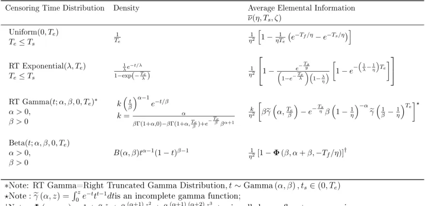
Table 3.2: The expected elemental information matricesν(Te, Ts, η)for the dierent distribution of censoring time Tf =Ts−t, for exponential distributed lifetime
Censoring Time Distribution Density Average Elemental Information
ν(η, Ts, ζ)
Uniform(0, Te)
Te≤Ts
1 Te
1 η2
h 1−ηT1
e e
−Tf/η−e−Ts/η i
RT Exponential(λ, Te)
Te≤Ts
1 λe
−t/λ 1−exp(−Te
λ)
1 η2
1− e −Tsy
1−e−Teλ
1−λ η
1−e−
1 λ− 1 η Te
RT Gamma(t;α, β,0, Te)∗
α >0, β >0
kβtα−1e−t/β
k= α
βΓ(1+α,0)−βΓ(1+α,Teβ)+e− Te
β βα+1 k η2
βγe
α,Te β
−e−Tsη β
1−1η−αeγ
1 β −
1 η
Te?
Beta(t;α, β,0, Te)
α >0, β >0
B(α, β)tα−1(1−t)β−1 η12 [1−Φ(β, α+β,−Tf/η)]
†
∗Note: RT Gamma=Right Truncated Gamma Distribution, t ∼Gamma(α, β), ts ∈(0, Te) ?Note:eγ(α, z) = ´0ze−ttt−1dtis an incomplete gamma function;
†Note:Φ(α, ω;z) = 1 +αω1!z +αω((αω+1)+1)z2!2 +αω((αω+1)+1)((ωα+2)+2)z3!3 +...is called a conuent hypergeometric function.
.
3.4 Properties and numerical procedures
3.4.1 Properties of locally optimal designs
As soon as elemental matrix (3.46) is found the entire machinery of optimal design the-ory can be implemented to address optimization problem. We will follow the generalized approach proposed in Atkinson et al. (2012), and Fedorov and Leonov (2014).
The most dicult part of (3.50) is the search of design ξ∗ that minimizes a selected criterion of optimality:
ξ∗ = arg min
ξ Ψ [M(ξ, Te, Tf)], (3.51) Assuming that Ψ[M] is monotonic, i.e.Ψ[m]≥Ψ[m0], m≥m0, and homogeneous, i.e.Ψ[cm] = γ(c)Ψ[m], one can verify that given Te and Tf,
ξ∗ = arg min
ξ Ψ [M(ξ, Te.Tf)]. (3.52)
Note that unlike the standard case where the locally optimal design depends on estimated parameters θ, the design ξ∗ dened by (3.52) depends onθ, Te, and Tf. Let
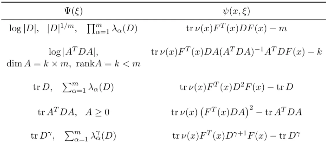
ψ(x, ξ) = lim α→0
Ψ [(1−α) M(ξ) +αµ(x)]
α (3.53)
This function is often called sensitivity function and presented in Table 3.3. In this table we skipped θ in ν(x, θ) and F(x, θ) for a few most popular criteria. Under rather mild assumptions (mainly convexity of Ψ(M)), the following hold:
1. There exists an optimal design ξ∗ that contains no more than m(m + 1)/2 support points, m= dimθ.
Table 3.3: Sensitivity functionsψ(x, ξ), D=M−1
Ψ(ξ) ψ(x, ξ)
log|D|, |D|1/m, Qm
α=1λα(D) trν(x)FT(x)DF(x)−m
log|ATDA|, trν(x)FT(x)DA(ATDA)−1ATDF(x)−k
dimA=k×m, rankA=k < m
trD, Pmα=1λα(D) trν(x)FT(x)D2F(x)−trD
trATDA, A≥0 trν(x) FT(x)DA2
−trATDA
trDγ, Pmα=1λγα(D) trν(x)FT(x)Dγ+1F(x)−trDγ
3. A necessary and sucient condition for ξ∗ to be optimal is the inequality
min x∈X ψ(x, ξ
∗
)≥0, (3.54)
X is a set of all admissible x.
4. Function ψ(x, ξ∗)equals zero at all supported points of ξ∗.
Traditionally, the combination of statements1−4 is called equivalence theorem. All of papers cited in section 3.1 are focused on derivation of statements 3 and 4 for their very specic cases.
We would like to emphasize that 1-4 contain nothing new comparatively to what was discussed in Atkinson et al. (2012), and Fedorov and Leonov (2014) except the very spe-cial structure of the information matrices µ(x) of a single observation performed at x or more fundamentally, except the structure of the elemental information matrices ν.
3.4.2 Numerical procedures
construc-observation as they dened in the above references and mainly following the track of the previous section a reader can easily modify the rst order algorithms (Fedorov and Leonov 2014, Ch 3-6). The respective R codes can be requested from the authors.
Unlike to the standard optimal design where the optimal support points (in our case dose) and respective number of observations should found optimization problem (3.50) has global controls like total enrolment rate λ duration of enrolmentTe and follow up period Tf. Usually function C(λ, Te, Tf) is increasing with respect to all three variables and in the simplest case is linear.
C(λ, Te, Tf) =c0+C1λ+C2Te+C3Tf =C∗. (3.55) Inequality in (3.50) can be replaced by equality due to monotonicity of Ψ[M] and the fact elemental information matrix increases (Loewner's sense) as a functionTe and Tf, see Ta-ble 3.2. Note that the potential loss of future revenues is not included in (3.55) and that can change the problem dramatically. In the case of block busters one has to nish trial as soon as nancially and technically possible and satisfy medicine ethical or regulatory constraints.
Using (3.55) we may exclude one of global controls. Often Tf is dened from medical considerations and we end up with the following one dimension optimization problem
{ξ∗, Te∗, λ∗} = arg min Te
(α−βTf)TfΨ [M(ξ∗(Te, Tf), Te, Tf)], (3.56)
λ = C
∗−C
0−C2Tf −C3Te C1
,
where α = C∗−C0−C3Tf
3.5 Example
In this section we consider the most popular model in clinical trials: exponentially dis-tributed time-to-event, i.e.
φ(t, η) =η−1e−t/η, h(t, η) = η−1, Φ(t, η) = 1−e−t/η, (3.57)
see also Table 3.1. This model can be viewed as the simplest example of a proportional hazard model, which is rather simple on its own. Indeed from (3.30) it immediately follows that for any proportional hazard model for observations censored atT
ν(T, η) = 1
η2Φ(T, η), (3.58)
and for the enrolment that can be modelled by a homogeneous Poisson process
ν(Te, T −f, η) = 1 η2
ˆ Te
0 1 Te
Φ(Te+Tf −t)dt, (3.59)
In a few cases integration can be done analytically see Table 3.2 for examples. Otherwise it can be performed numerically.
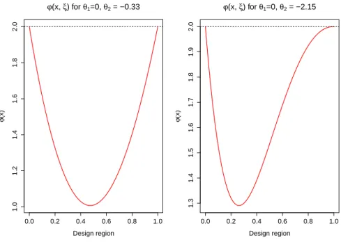
Let us start with D-Criterion: Ψ[M] = −ln|M|. For the slow changing functionw(x) D-optimal design allocate subjects at extreme dosesx∗1 = 0, and x∗2 = 1 with equal weights p1 = p2 = 0.5, see for instance see for instance Fedorov (1972). D-optimality of that design can be easily veried using the equivalence theorem and the fact ψ(x, ξ) = w(x)f>(x)M−e(ξ)f(x)−m. See also Figure 3.2, left panel where function
of hazard forx = 1 and x = 0) would be extremely potest. Starting from this value opti-mal dose x∗2 moves towards smaller doses, compare with similar results from Muller (2013) that were derived from xed censoring.
0.0 0.2 0.4 0.6 0.8 1.0
1.0
1.2
1.4
1.6
1.8
2.0
Design region
ϕ
(x)
ϕ(x, ξ) for θ1=0, θ2 = −0.33
0.0 0.2 0.4 0.6 0.8 1.0
1.3
1.4
1.5
1.6
1.7
1.8
1.9
2.0
Design region
ϕ
(x)
ϕ(x, ξ) for θ1=0, θ2 = −2.15
Figure 3.2: Sensitivity analysis
3.6 Conclusion
CHAPTER 4: RAPID ENROLLMENT DESIGN FOR FINDING THE OPTIMAL DOSE IN IMMUNOTHERAPY TRIALS WITH ORDERED
GROUPS
4.1 Introduction
proba-In some dose-nding trials the patient population consists of two or more subpopu-lations with possibly dierent susceptibility to toxicity. For example, adults and kids, or subpopulations with dierent genotypes. For example, Inocenti et al. (2004) suggested that U GT1A1 genotype predicts the occurrence of severe neutropenia during irinotecan therapy. Patients with the TA indel 7 of 7 genotype had much higher risk of developing grade four neutropenia than other patients Innocenti et al. (2004). Such trials are referred to as trials in ordered groups. O'Quigley and Paoletti (2003) proposed a modication of the continual reassessment method (CRM) for trials with ordered groups. Ivanova and Wang (2006) proposed an up-and-down design for ordered groups where the order among the groups is modeled using isotonic regression. Patients in dierent subgroups, in addi-tion to having dierential toxicity, can have dierent probabilities of responding at a given dose.
ordered groups. Ivanova et al. (2016) proposed a more conservative approach than the one used in TITE-CRM to handle potential future toxicity in patients still in follow-up. The rapid enrollment design (RED) Ivanova et al. (2016) is a Bayesian dose-nding design that allows imputing potential toxicities from patients still in follow-up with the decision rule regarding what does to assign to the next patient.
In this paper we extend the RED to the problem of nding the optimal dose and show how to apply the new design to dose-nding in ordered groups. This work was motivated by an ongoing dose-nding trial of autologous chimeric antigen receptor modied T cells (CAR-T cells) in patients with acute lymphoblastic leukemia. In this case, a molecular safety switch can be triggered by a small molecule. Since little or no toxicity was experi-enced by subjects in other trials of this small molecule Zhou et al. (2015), in this trial the target dose of the small molecule was dened as the dose where the probability of thera-peutic response (improvement in cytokine release syndrome) without toxicity is maximized among doses with the probability of toxicity of at most 0.25. After a safety phase, patients are enrolled in two separated cohorts: pediatric (from 3 to 18 years old) and adult (>18 years old). Pediatric patients show higher tolerance for the CAR-T cells as compared to adult patients, hence we assume that the probability of unacceptable CAR-T cell toxicity in adult population is more than or equal to the probability of such toxicity in pediatric patients treated with the same CAR-T cell dose.
4.2 Estimating under order restrictions
4.2.1 Notation
Each patient is followed for toxicity and response for a xed period of time. Let T1 be the length of follow-up for toxicity, and T2 be the length of follow-up for response. Toxic-ity and responses observed outside the observation window do not count. With regard to toxicity (T) and therapeutic response (R), there are four possible outcomes: no response and no toxicity, T−R−, response and no toxicity, T−R+, no response and toxicity, T+R−,
and response and toxicity, T+R+. Let groups 1, 2, · · · , I be the sub-populations with dif-ferent susceptibility to toxicity. For a subject in group i, i= 1,· · ·, I, assigned to dose k =1,2,· · · , K denote πik1 = Pr(T−R−),πik2 = Pr(T−R+),πik3 = Pr(T+R−), and πik4 = Pr(T+R+). Observations from dierent subjects are independent. Let{y
ik1, yik2, yik3, yik4} be the number of patients out of nik =
P4
l=1yikl with outcomes T−R−, T−R+,T+R−, and T+R+, correspondingly, at dose k, k =1,2, · · ·, K, and in group i,i =1, 2, · · · , I. Fur-ther denote the number of patients with positive Fur-therapeutic response by y0ik2 =yik2+yik4, and the number of patients with toxicity by yik0 3 = yik3 +yik4. Let π0ik2 = πik2 +πik4 be the probability of response and πik0 3 = πik3 +πik4 be the probability of toxicity. The vec-tor of counts(yikl, yik2, yik3, yik4) follows multinomial distribution with parameters nik and (πikl, πik2, πik3, πik4).
4.2.2 Isotonic estimation of toxicity and response probabilities in a trial with ordered groups
Since y1 = (y11l, y12l· · · , y1Kl), follows multinomial distribution the likelihood is
L(y1l,y2l,· · · ,yIl,|π1l,π2l,· · · ,πIl) = I
Y
i=1 K
Y
k=1 4
Y
l=1
(πik1, πik2, πik3, πik4). The Dirichlet is the conjugate prior for multinomial distribution with posterior distribution computed as
(πik1, πik2, πik3, πik4|yik1, yik2, yik3, yik4)∼
Dirichlet(yik1 +α1, yik2+α2, yik3+α3, yik4+α4). (4.61)
To use the information on monotonicity of response and toxicity in dose within each group and the order between the groups, we use the Bayesian isotonic transformation (Dun-son and Neelon, 2003), to project from R3×I×K into the restricted space Ω using a minimal distance mapping, where Ω∈ R3×I×K is dened by set of vectors of multinomial probabili-ties such that
1. πi013 ≤π0i23≤ · · · ≤πiK0 3, i= 1,2,· · ·, I;
2. πi012 ≤π0i22≤ · · · ≤πiK0 2, i= 1,2,· · ·, I; 3. π10k3 ≥π20k3 ≥ · · · ≥πIk0 3,k = 1,2,· · · , K;
4. π10k2 ≤π20k2 ≤ · · · ≤πIk0 2,k = 1,2,· · · , K; (62)
Following Dunson and Neelan (2003), the Bayesian isotonic transformation is obtained by drawing samples from the posterior distribution of unconstrained parameter vectors (π∗ik1, πik∗2, πik∗3, πik∗4),k = 1,2,· · · , K, i = 1,2,· · · , I. Then we calculate the number of each of the four outcomes at each dose levelk within each group i that correspond to the draw as y˜ikl = P4l=1yikl+P4l=1αl
∗πikl. The draw is transformed to the constrained∗
space by maximizing the likelihood Π = supˆ QI
i=1
QK
k=1
Q4
l=1(πikl) ˜
yikl under restrictions (i),(ii),(iii),(iv) in (62).
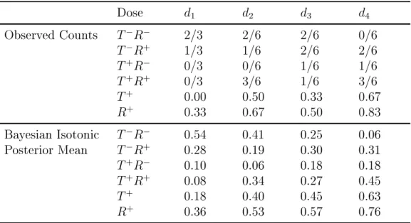
4.3 Examples
We illustrate the computation described in Section 4.2 by two examples. We maxi-mized the likelihood by using an optimization routine constrOptim in R software (R Core Team). The rst example is a hypothetical example with a single group and 4 dose levels after 21 patients have been assigned. 4.4 displays the observed counts in the 4 cells of the 2x2 table for each dose and observed proportions or responses and toxicities. We present posterior means after the Bayesian isotonic transformation Dunson and Neelon (2003), with Dirichlet prior with parameters (0.5, 0.5, 0.5, 0.5). We present posterior means of transformed variables under the order constraints on the probability of toxicity π013 ≤
π230 ≤ π330 ≤ π430 and the probability of therapeutic response π120 ≤ π022 ≤ π320 ≤ π042. We used a Dirichlet prior with parameters (0.5, 0.5, 0.5, 0.5).
Table 4.4: An example of Bayesian isotonic estimation in a single group. Observed counts are presented as the number of outcomes over the total number of patients at the dose
Dose d1 d2 d3 d4
Observed Counts T−R− 2/3 2/6 2/6 0/6
T−R+ 1/3 1/6 2/6 2/6
T+R− 0/3 0/6 1/6 1/6
T+R+ 0/3 3/6 1/6 3/6
T+ 0.00 0.50 0.33 0.67
R+ 0.33 0.67 0.50 0.83
Bayesian Isotonic T−R− 0.54 0.41 0.25 0.06
Posterior Mean T−R+ 0.28 0.19 0.30 0.31
T+R− 0.10 0.06 0.18 0.18
T+R+ 0.08 0.34 0.27 0.45
T+ 0.18 0.40 0.45 0.63
R+ 0.36 0.53 0.57 0.76
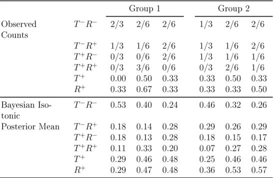
An example with two ordered groups is displayed in the Table 2, where 42 subjects, 21 in group 1 and 21 in group 2, have been assigned to 3 dose levels. The Bayesian isotonic transformation estimates are calculated under the assumption that both toxicity and ther-apeutic response are monotone with dose within each group. Additionally, we assume that at each dose toxicity is higher in group 1 compared to group 2, restriction c) of (1), and response in group 1 is lower compared to group 2, restriction d) in (1).
4.4 The rapid enrollment design to nd the optimal doses in two ordered groups
Table 4.5: An example of Bayesian isotonic estimation under constrains in (1) in two groups. Observed counts are presented as the number of outcomes over the total number of patients at the dose
Group 1 Group 2
Observed Counts
T−R− 2/3 2/6 2/6 1/3 2/6 2/6
T−R+ 1/3 1/6 2/6 1/3 1/6 2/6
T+R− 0/3 0/6 2/6 1/3 1/6 1/6
T+R+ 0/3 3/6 0/6 0/3 2/6 1/6
T+ 0.00 0.50 0.33 0.33 0.50 0.33 R+ 0.33 0.67 0.33 0.33 0.33 0.50 Bayesian
Iso-tonic
T−R− 0.53 0.40 0.24 0.46 0.32 0.26
Posterior Mean T−R+ 0.18 0.14 0.28 0.29 0.26 0.29 T+R− 0.18 0.13 0.28 0.18 0.15 0.17
T+R+ 0.11 0.33 0.20 0.07 0.27 0.28 T+ 0.29 0.46 0.48 0.25 0.46 0.46 R+ 0.29 0.47 0.48 0.36 0.53 0.57
sucient number of patients assigned.
The proposed design to nd the optimal dose can be viewed as an extension of the rapid enrollment design (Ivanova et al., 2016). Below we describe the new rapid enrollment design for optimal dose (REDO) applied to a single group. Let 1· · ·, k be the set of doses
with at least one patient assigned.
1. Initial escalation. Do not change the dose unless at least m patients are assigned to a dose and their toxicity outcomes are observed (except when the safety rule is in-voked). We recommend using cohorts of m = 3. Assigning at least 3 patients pre-vents from making a decision based on insucient information.
2. If πˆk1 > πˆ0k3 and at least m patients are assigned to dose k, the next patient is as-signed to dose k+ 1 (or k if k =K).
3. if πˆk1 ≤ ˆπ0k3 and if there is a dose s such that πˆs1 = ˆπs03, the next patient is assigned to dose levels. Otherwise let s(s ≤ k −1) be such thatπsˆ 1 > πˆ0s3 and ˆπ(0s+1)3 > ˆ
π(s+1)1. That is, given the data, the optimal dose is somewhere between dose levels s and s + 1. Let the probability γs reect how close is the dierenceπˆis0 3 − ˆπis1 is to0, γs = Pr{− < ˆπ0s3 −πˆs1 < }. The next patient is assigned to the s∗ where s∗ = arg max(γs, γs+1), that is to the dose corresponding to the higher value of γs or γs+1.
4. Safety rule. Do not assign patients to dose with Pr(πk03 > Γ) > 0.9, i = 1,2, k = 1,2,· · · , K If Pr(π130 > Γ) > 0.9, the trial is stopped because the lowest dose is too toxic.
6. Estimation of the optimal dose at the end of the trial. Let N be the total sample size in the trial divided by the number of doses. That is, N is the average number of sub-jects assigned to a dose. At the end of the trial compare proportions of successes at the doses with at least N subjects assigned. The dose with the highest estimated probability of success and tolerable toxicity rate according to the safety rule 5) is declared the optimal dose. No dose is selected if the lowest dose is deemed too toxic by the safety rule 5).
4.5 Migrating for delayed toxicity and clinical response