Passive, automatic detection of network server performance anomalies in large networks

(1)

Passive, automatic detection of network server performance

anomalies in large networks

Jeff Terrell

A dissertation submitted to the faculty of the University of North Carolina at Chapel Hill in partial fulfillment of the requirements for the degree of Doctor of Philosophy in the Department of Computer Science.

Chapel Hill 2009

Approved by:

Kevin Jeffay, Advisor

F. Donelson Smith, Reader

Ketan Mayer-Patel, Reader

Vern Paxson, Reader

(2)

c

2009

Jeff Terrell

(3)

Abstract

JEFF TERRELL

Passive, automatic detection of network server performance anomalies in large networks

(Under the direction of Kevin Jeffay.)

“Network management” in a large organization often involves—whether explicitly or implicitly— the responsibility for ensuring the availability and responsiveness of network resources attached to the network, such as servers and printers. Users often think of the services they rely on, such as web sites and email, as part of “the network”. Although tools exist for ensuring the availability of the servers running these services, ensuring their performance is a more difficult problem.

In this dissertation, I introduce a novel approach to managing the performance of servers within a large network broadly and cheaply. I continuously monitor the border link of an enterprise network, building for each inbound connection an abstract model of the application-level dialog contained therein without affecting the operation of the server in any way. The model includes, for each request/response exchange, a measurement of theserver response time, which is the fundamental unit of performance I use. I then aggregate the response times for a particular server into daily distributions. Over many days, I use these distributions to define a profile of the typical response time distribution for that server. New distributions of response times are then compared to the profile to determine whether they are anomalous.

I applied this method to monitoring the performance of servers on the UNC campus. I tested three months of continuous measurements for anomalies, for over two hundred UNC servers. I found that most of the servers saw at least one anomaly, although for many servers the anomalies were minor. I found seven servers that had severe anomalies corresponding to real performance issues. These performance issues were found without any involvement of UNC network managers, although I verified two of the issues by speaking with network managers. I

(4)

(5)

To the dearest and best, the Lord Jesus Christ. You are my rock.

(6)

Acknowledgments

(7)

List of Tables

3.1 essential state for a segment record in adudump . . . 34

3.2 connection identifier structure . . . 34

3.3 essential per-connection state in adudump . . . 35

3.4 essential per-flow state inadudump . . . 35

3.5 the types of records output byadudump . . . 52

3.6 adudump output format for an example connection . . . 53

3.7 Dataset 1: adudump measurements from border link . . . 53

3.8 Dataset 2: adudump measurements from border link . . . 53

6.1 iterations of filtering Nagios records . . . 175

6.2 iterations of filtering Nagios records (continued) . . . 176

6.3 salient information from service performance alert records . . . 177

6.4 remaining Nagios issues . . . 184

6.5 unmatched anomalies identified by my methods . . . 207

(10)

List of Figures

2.1 TCP steady-state operation. (a) shows the sequence numbers of the data, the packets in transit, and the state of the connection just before packets A (an acknowledgement) and B (data) are received. (b) shows the state of

the network afterward; note that the sender’s window has advanced. . . 18

2.2 the A–B–T model, consisting of A-type objects, B-type objects, and think-times. The bottom connection shows two data units separated by an

intra-unit quiet time. . . 21

3.1 Placement of the monitor with respect to the UNC network . . . 29

3.2 One-pass A–B–T connection vector inference example. The details of the

connection close have been omitted. . . 31

3.3 Round-trip-time measurements of the TCP handshake for inbound connections. 33

3.4 Sequential validation results . . . 50

3.5 Concurrent validation results . . . 51

4.1 Example histogram for an example server, with bins divided equally

ac-cording to a logarithmic scale. . . 60

4.2 Interpolations between two Gaussian distributions (one red, one blue), shown upper-left. PDF interpolation, upper-right. CDF interpolation and the corresponding PDFs (middle row). QF interpolation and the

corre-sponding PDFs (bottom row). From [Bro08]. . . 63

4.3 Distributions of response time measurements using aPDF and aCDF

rep-resentations. . . 65

4.4 Quantile function representation and singular values of PCA using various

representations. . . 65

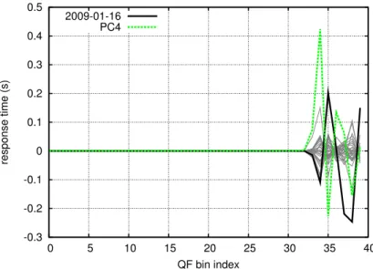
4.5 Quantile functions for example server, plotted on a logarithmic scale, with

the anomalous QF highlighted . . . 71

4.6 The zero-centered quantile functions, with principal component 1 . . . 72

4.7 The projection of each QF onto principal component 1 . . . 73

4.8 Residual 1: the leftover of each QF, after subtracting its respective

projec-tion onto PC 1 from the QF itself . . . 74

(11)

4.10 Residual 2: the leftover after subtracting the first and second projections

from each QF . . . 75

4.11 The projection of each residual 2 onto PC 3 . . . 76

4.12 Residual 3: the leftover after subtracting the first through the third pro-jections from each QF . . . 77

4.13 The projection of residual 3 onto PC 4 . . . 77

4.14 Residual 4: the leftover after subtracting projections 1–4 . . . 78

4.15 The projection of residual 4 onto PC 5 . . . 78

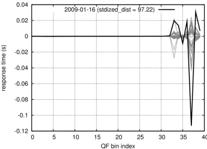
4.16 Residual 5: the final residual after subtracting the projection of each QF into the PCA-defined normal subspace . . . 79

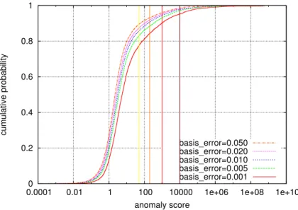
4.17 Anomaly scores asbasis errorvaries, for all the servers in the corpus. . . . 83

4.18 Anomaly scores aswindow sizevaries, for all the servers in the corpus. . . . 84

4.19 Anomaly scores astset sizevaries, for all the servers in the corpus. . . 85

4.20 Anomaly scores asnum bins varies, for all the servers in the corpus. . . 86

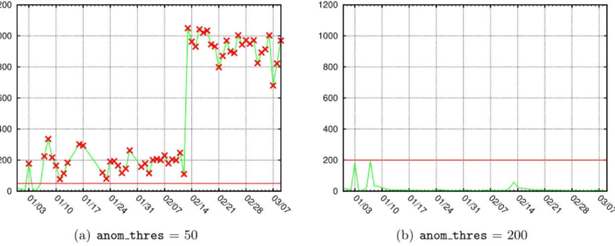
4.21 Anomaly scores for an example server at different settings of anom thres . . 87

4.22 Anomaly scores asanom thres varies, for all the servers in the corpus. . . 87

4.23 Quantile-Quantile plot of projection along first principal component for an example server. The projection is quite non-Gaussian. . . 88

4.24 Median anomaly score asbasis errorand window size vary . . . 91

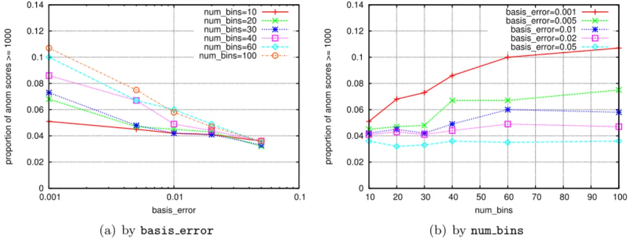
4.25 Proportion of anomaly scores greater than or equal to 1000, asbasis error and window size vary . . . 91

4.26 Median anomaly score asbasis errorand tset size vary . . . 93

4.27 Proportion of anomaly scores greater than or equal to 1000, asbasis error and tset sizevary . . . 93

4.28 Median anomaly score asbasis errorand num bins vary . . . 94

4.29 Proportion of anomaly scores greater than or equal to 1000, asbasis error and num bins vary . . . 94

4.30 Median anomaly score asbasis errorand anom thres vary . . . 95

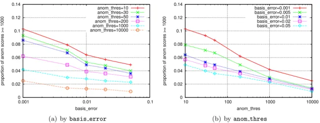
4.31 Proportion of anomaly scores greater than or equal to 1000, asbasis error and anom thres vary . . . 95

4.32 Median anomaly score aswindow sizeand tset size vary . . . 96

(12)

4.33 Proportion of anomaly scores greater than or equal to 1000, aswindow size

and tset sizevary . . . 96

4.34 Median anomaly score aswindow sizeand num bins vary . . . 97

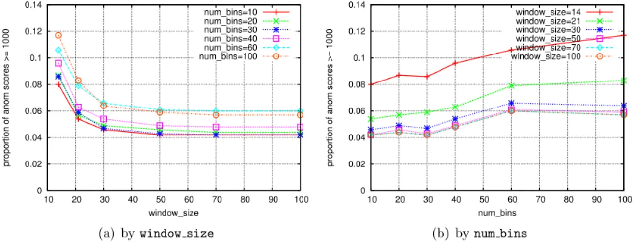
4.35 Proportion of anomaly scores greater than or equal to 1000, aswindow size and num bins vary . . . 97

4.36 Median anomaly score aswindow sizeand anom thres vary . . . 98

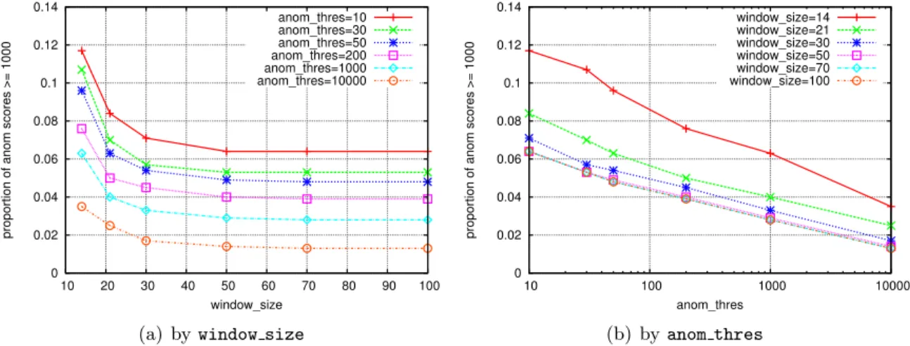
4.37 Proportion of anomaly scores greater than or equal to 1000, aswindow size and anom thres vary . . . 98

4.38 Median anomaly score astset sizeand num bins vary . . . 99

4.39 Proportion of anomaly scores greater than or equal to 1000, astset size and num bins vary . . . 99

4.40 Median anomaly score astset sizeand anom thres vary . . . 100

4.41 Proportion of anomaly scores greater than or equal to 1000, astset size and anom thres vary . . . 100

4.42 Median anomaly score asnum bins andanom thres vary . . . 101

4.43 Proportion of anomaly scores greater than or equal to 1000, as num bins and anom thres vary . . . 101

4.44 Anomaly score for web server. Outages resulting in incomplete days are represented by breaks in the line. . . 103

4.45 Time-scale analysis for web server on quarter-day distributions. . . 104

4.46 Time-scale analysis for web server on hourly distributions. . . 105

4.47 Time-scale analysis for web server on rolling-day distributions. . . 106

4.48 Anomaly score for an SMTP server. . . 108

5.1 Anomaly score for teleconferencing server on a logarithmicallscaled y-axis. The labeled days on the x-axis are Saturdays. . . 113

5.2 The time-scale analysis for the teleconferencing server with a rolling-day basis. 113 5.3 Selected distributions ofcriticalanomalies for the teleconferencing server, plotted on a logarithmic x-axis. . . 114

(13)

5.5 The number of SYN(SEQ) records, or connection attempts (connection es-tablishments), reported byadudumpper day for the teleconferencing server. The color of the X indicates the anomaly classification of that day. Days without an X are from the training set, and the grey X’s mark the days

rejected by the bootstrapping process. Breaks in the line represent outages. . 115

5.6 The number of ignored (or dropped) connections and the number of rejected

connections for the teleconferencing server, per day. . . 116

5.7 The number of request ADU records reported by adudump per day for the

teleconferencing server. . . 117

5.8 The anomaly score as a function of demand for the teleconferencing server,

using three different demand measures. . . 117

5.9 The anomaly score for the teleconferencing server as a function of failed

connection attempts. . . 118

5.10 The number of unique client addresses per day for the teleconferencing server. 118

5.11 The number of open connections at the beginning of each hour in a normal and an anomalous slice of traffic. The anomalous slice was translated so

that it could be plotted alongside the normal slice. . . 119

5.12 Anomaly score for POP3 server on a logarithmically-scaled y-axis. The

labeled days on the x-axis are Saturdays. . . 120

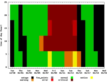
5.13 Anomaly score heat-map with a rolling-day time-scale for the POP3 server. . 121

5.14 Distributions of response times leading tocriticalanomalies. . . 121 5.15 The number of SYN (SEQ) records, or connection attempts (connection

establishments), reported by adudump per day for the POP3 server. The color of the X indicates the anomaly classification of that day. Days without

an X are from the training set. Breaks in the line represent outages. . . 122

5.16 Number of request ADUs per day for the POP3 server. . . 123

5.17 Number of rejected connection attempts (a), and the number of unique

client addresses rejected (b), per day, for the POP3 server. . . 123

5.18 CDFs of connection durations in the normal period, anomalous period, and anomalous period with host H removed. Connection durations are taken by subtracting the timestamp of theSYNrecord from the timestamp of the

ENDrecord reported by adudump. . . 124 5.19 Percentage of connections having at leastX exchanges for the POP3 server. . 125

5.20 Median response time by ordinal for the normal and anomalous periods, with 5% and 95% error bars, for the POP3 server. For example, the point (and bars) at X= 2 represents the distribution of response times that occur

for the second request/response exchange within their respective connection. 126

(14)

5.21 Median request and response size by ordinal for the normal and anomalous

periods, with 5% and 95% error bars, for the POP3 server. . . 126

5.22 Anomaly score for portal server. Outages resulting in incomplete days are

represented by breaks in the line. Dates are 2008. . . 130

5.23 Training set (gray lines) and response time distributions for portal server. . . 131

5.24 Training set (gray lines) and response time distributions for portal server. . . 132

5.25 Results from a structural analysis of the portal server . . . 132

5.26 Results from a structural analysis of the portal server . . . 133

5.27 Anomaly score for campus SMTP server. Outages resulting in incomplete

days are represented by breaks in the line. Dates are 2009. . . 134

5.28 Distributions of response times both for normal operation (black lines) and selected anomalous distributions (colored lines), plotted on a logarithmic scale, for the campus SMTP server. Note that the anomaly on March 5 is

only a erroranomaly (i.e. with a score between 1,000 and 10,000). . . 134 5.29 Number of unique IP addresses per day initiating a connection with the

SMTP server. . . 135

5.30 Count and total size of request and response ADUs per day for the campus

SMTP server. . . 136

5.31 Connection duration for normal vs. anomalous weeks for campus SMTP server. 137

5.32 Open connections at the start of an hour for SMTP server, for normal week

vs. anomalous week. . . 138

5.33 Connection attempts and failed connection attempts per day for the campus

SMTP server . . . 139

5.34 Scatter plot of request sizes vs. response times, for a normal week and an anomalous week. Note: the anomalous week is sampled at a rate of 1/100,

and the normal week is sampled at a rate of 1/10,000. . . 140

5.35 Response time CDFs for campus SMTP server, split by whether the

corre-sponding request was greater than or less than 600 bytes. . . 140

5.36 Time-scale analysis for SMTP server on rolling-day distributions. . . 141

5.37 Anomaly score for SMTP server during the onset of the performance issue. . 142

5.38 Average response time, and count of responses, per hour, for SMTP server

during the onset of the anomalous behavior. . . 143

(15)

5.40 Manually selected training set: all days through Feb. 9 are included. The

heavier distributions occur after the traffic shift on February 3rd_{. . . .} ₁₄₅

5.41 New anomaly timeseries, after resetting the basis. . . 145

5.42 Normal and anomalous distributions after resetting the basis. Only two distributions were flagged as anomalous, and (despite the color) they were only noticeanomalies. Thus, many of the previously anomalous

distribu-tions are now considered normal. . . 146

5.43 Anomaly score for departmental web server. Outages resulting in

incom-plete days are represented by breaks in the line. Dates are 2009. . . 147

5.44 Distributions of response times for normal operation (black lines) and an-omalous operation (colored lines). The first three colored lines are from

theerror period, and the last two lines are from thecriticalperiod. . . 147 5.45 The number of connection attempts per day for the departmental web server. 148

5.46 The number of connection attempts that were rejected or ignored per day

for the departmental web server. . . 148

5.47 Count and total size of request/response ADUs per day for the

departmen-tal web server. . . 149

5.48 The number of open connections at the start of an hour for both the normal

and error period of the departmental web server. . . 149

5.49 The number of response times and average response time per day for the

departmental web server. . . 150

5.50 The request size for the departmental web server shifts on February 7, 2009. . 150

5.51 Results from an ordinal analysis of the normal period versus the “error”

period for the departmental web server. . . 151

5.52 The median request and response sizes, with 5/95 percentile error bars, by

ordinal, for the normal and “error” periods of the departmental web server. . 152

5.53 Results from an ordinal analysis of the normal period versus the “error”

period versus the “critical” period for the departmental web server. . . 153

5.54 The median request and response sizes, with 5/95 percentile error bars, by ordinal, for the normal, “error”, and “critical” periods of the departmental

web server. . . 153

5.55 Anomaly detection results with a rolling-day time-scale for the

5.56 Anomaly detection results with a rolling-day time-scale for the

(16)

5.57 Anomaly score for departmental SMTP server. Outages resulting in

in-complete days are represented by breaks in the line. Dates are 2009. . . 156

5.58 Distributions of response time distributions for normal operation (black

lines) and anomalous operation (colored lines). . . 156

5.59 Results from an ordinal analysis of the normal period versus the anomalous

period for the departmental SMTP server. . . 157

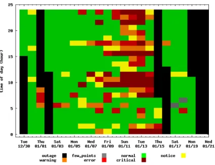
5.60 Anomaly detection results as a heat-map with a rolling-day time-scale for

campus SMTP server. . . 158

5.61 Anomaly score for the unknown service. Outages resulting in incomplete

days are represented by breaks in the line. Dates are 2009. . . 159

5.62 Normal response time distributions (black) and critical response time

distributions (colored) for the unknown service. . . 159

5.63 Number of unique clients attempting a connection per day, and the number of total connection attempts for the unknown service, both plotted versus

the anomaly score. . . 160

5.64 Connection establishments and connection failures per day for the unknown

service, both plotted versus the anomaly score. . . 160

5.65 Number of requests per day for the unknown service versus the anomaly score. 160

5.66 Comparisons between normal and anomalous periods for the unknown service. 161

5.67 Median response time, with Q1/Q3 error bars, for the response times by

ordinal for the unknown service. . . 161

5.68 Anomaly detection results for the unknown service, both overall and for

the first ordinal only. . . 162

5.69 Anomaly detection results for the unknown service for the second and third

ordinal. . . 162

5.70 Median request/response size, with Q1/Q3 error bars, by ordinal, for the

unknown service. . . 162

5.71 Number of connection rejections for both services on the unknown service. . . 163

5.72 Time, in seconds, between a particular client contacting either service. . . 163

5.73 Anomaly score timeseries for both services. . . 164

5.74 Highlighted response time distributions for both services. . . 164

5.75 Proportion of connections having at least X exchanges, in both services,

(17)

5.76 Proportion of connections having at least X exchanges, in both services,

for both a normal period and an anomalous period. . . 166

5.77 Number of unique clients attempting a connection per day, and the number of total connection attempts for the unknown service, both plotted versus

the anomaly score. . . 166

5.78 Connection establishments and connection failures per day for the unknown

service, both plotted versus the anomaly score. . . 166

5.79 Number of requests per day for the unknown service versus the anomaly score. 167

5.80 The anomaly detection results with a rolling-day timescale for the non-acad

server. . . 168

5.81 The quarter-hour response time distributions prior to the anomalous dis-tribution (black), and the quarter-hour anomalous disdis-tribution (red), for

the non-acad server. . . 169

6.1 Count of response time measurements for beta server around the time of

its only issue. . . 179

6.2 Count of response time measurements for alphaserver around the time of

its first issue. . . 179

its second and third issues, which were separated by 18 minutes. . . 180

its fourth and fifth issues, which were separated by 37 minutes. . . 180

6.5 Count of response time measurements for alphaserver around the time of its sixth through ninth issues. The sixth and seventh issues were separated

by 27 minutes, and the seventh and eighth issues were separated by 12 minutes. 181

6.6 Count of response time measurements for alpha server around the time of its 10th through 16th issues, which were separated by 72 minutes, 12

minutes, 5 minutes, 20 minutes, 5 minutes, and 82 minutes, respectively. . . . 181

6.7 Count of response time measurements for alpha server around the time of its 17th _{through 23}rd _{issues, which were separated by 72 minutes, 17}

minutes, 5 minutes, 5 minutes, 15 minutes, and 5 minutes, respectively. . . . 182

its 24th _{and 25}th _{issues, which were separated by 32 minutes. . . .} ₁₈₂

6.9 Count of response time measurements for gammaserver around the time of

6.10 Count of response time measurements per day forgammaserver. . . 185

(18)

6.11 Count of response time measurements fordeltaserver around the time of

6.12 Average response time per hour for delta server around the time of its

only issue. . . 186

6.13 Count of response time measurements forepsilonserver around the time

of its first issue. . . 187

6.14 Average response time per hour forepsilon server around the time of its

first issue. . . 187

6.15 Count of response time measurements per day forepsilonserver. . . 188 6.16 Daily anomaly score for theepsilon server. . . 188 6.17 Response time distributions for theepsilon server, with the distribution

containing its first issue highlighted. . . 189

of its second issue. . . 190

second issue. . . 190

6.20 Proportion of observed response times over the five second threshold per

hour bin for epsilonserver around the time of its second issue. . . 191 6.21 Response time distributions for the epsilon server, with the distribution

containing its second issue highlighted. . . 191

of its third issue. . . 192

third issue. . . 192

hour bin for epsilonserver around the time of its third issue. . . 193 6.25 Response time distributions for the epsilon server, with the distribution

containing its third issue highlighted. . . 193

6.26 Count of response time measurements per day forzetaserver. . . 194 6.27 Count of response time measurements for zeta server around the time of

6.28 Count of response time measurements foretaserver around the time of its

(19)

6.29 Average response time per hour foretaserver around the time of its only

issue. . . 196

hour bin for etaserver around the time of its only issue. . . 196 6.31 Proportion of observed response times over the five second threshold per

hour bin for etaserver. . . 197 6.32 Daily anomaly score for theetaserver. . . 197 6.33 Response time distributions for the etaserver, with the distribution

con-taining its only issue highlighted. . . 198

6.34 Count of response time measurements forthetaserver around the time of

6.35 Average response time per hour for theta server around the time of its

only issue. . . 199

hour bin for thetaserver around the time of its only issue. . . 200 6.37 Daily anomaly score for thetheta server. . . 200 6.38 Response time distributions for the theta server, with the distribution

containing its only issue highlighted. . . 201

6.39 Response time distributions for the theta server, with the distribution

6.40 Count of response time measurements per day foriotaserver. . . 202 6.41 Count of response time measurements for iota server around the time of

its two (simultaneous) issues. . . 203

6.42 Count of response time measurements forkappaserver around the time of

6.43 Average response time per hour for kappa server around the time of its

only issue. . . 204

hour bin for kappaserver around the time of its only issue. . . 204 6.45 Daily anomaly score for thekappa server. . . 205 6.46 Response time distributions for the kappa server, with the distribution

6.47 Count of response time measurements per day forlambdaserver. . . 206

(20)

6.48 Count of response time measurements for lambda server around the time

of its two (nearly simultaneous) issues. . . 206

6.49 Daily anomaly score for thezeta server. . . 208 6.50 Response time distributions for the zeta server, with the two anomalous

distributions highlighted. . . 208

6.51 Daily anomaly score for themu server. . . 209 6.52 Response time distributions for the mu server, with the first anomalous

distribution highlighted. . . 210

6.53 Response time distributions for themu server, with the second anomalous

6.54 Response time distributions for the mu server, with the third anomalous

6.55 Response time distributions for the mu server, with the fourth anomalous

6.56 Response time distributions for the mu server, with the fifth anomalous

6.57 Response time distributions for the mu server, with the sixth anomalous

day formu server, with anomalous days highlighted. . . 213 6.59 Proportion of observed response times over a twenty second threshold per

day formu server, with anomalous days highlighted. . . 213 6.60 Daily anomaly score for thenu server. . . 214 6.61 Response time distributions for the nu server, with the first anomalous

6.62 Response time distributions for thenu server, with the second anomalous

day fornu server. . . 215 6.64 Cumulative distribution function (CDF), zoomed, fornuserver, with

anom-alous distributions highlighted. Bin boundaries for a 40-bin QF are plotted

in red. . . 216

6.65 Cumulative distribution function (CDF), zoomed, on a log-scaled X-axis, fornuserver, with anomalous distributions highlighted. Bin boundaries for

(21)

6.66 Daily anomaly score for theomicron server. . . 218 6.67 Response time distributions for the omicron server, with the anomalous

day foromicron server. . . 219 6.69 Daily anomaly score for thepi server. . . 219 6.70 Response time distributions for the pi server, with the anomalous

distri-butions highlighted. . . 220

6.71 Daily anomaly score for therhoserver. . . 220 6.72 Response time distributions for therho server, with the anomalous

6.73 Daily anomaly score for thesigma server. . . 221 6.74 Response time distributions for thesigma server, with the anomalous

dis-tributions highlighted. . . 222

6.75 Daily anomaly score for thetauserver. . . 223 6.76 Response time distributions for thetau server, with the anomalous

6.77 Last four bins of the response time distributions for the tau server, with

the anomalous distributions highlighted. . . 224

A.1 Anomaly score timeseries for servers 1–3. Server 2 is used as an example in Section 4.7.5 of a server sensitive to the setting of anom thres. Server 3 is a portal web server for one of the colleges on campus (not the one mentioned in Chapter 5). During Jan 2–6, much fewer response times are less than 100 milliseconds than normal; however, the distribution is the same for response times greater than half a second, so it is likely that few users noticed a significant difference, despite theerrorand evencritical

anomaly scores. . . 232

A.2 Anomaly score timeseries for servers 4–6 . . . 232

A.4 Anomaly score timeseries for servers 10–12. Server 10 is an example of a server having too few response times to form a 40-bin QF for many of the days measured. As a result, bootstrapping occurs later, which is why many points show up as grey/black in the plot: the bootstrapping has not yet occurred, so a normal basis has not yet been formed. The last QF bin of server 12 is typically at most two seconds, yet between Jan 8–Feb 2, the

last two QF bins are both between 2–3 seconds. . . 233

(22)

A.17 Anomaly score timeseries for servers 49–51. Server 51 had a severecritical anomaly (with a score of over 8.8 million) on Feb 17, when the last QF bin jumped from its typical value of around 20–100 milliseconds to nearly 20 seconds. ITS reported that the cause of this problem was with the au-thentication component of the service, which had issues after a DNS server

outage. . . 237

A.18 Anomaly score timeseries for servers 52–54. Server 53 experienced a sus-tained performance anomaly starting on Feb 6, and lasting at least through

March 9. . . 237

A.22 Anomaly score timeseries for servers 64–66. Server 66 experienced a sus-tained performance issue from Jan 9–Feb 25, but it is a

dynamically-assigned address. . . 239

A.24 Anomaly score timeseries for servers 70–72. Server 71 experienced a per-formance issue starting on Mar 4 and continuing at least through Mar 9. Server 72 is one of many that were apparently shut down at some point

(23)

A.25 Anomaly score timeseries for servers 73–75. Server sockets 74 and 75 are

actually the same DHCP-assigned IP address. . . 240

A.28 Anomaly score timeseries for servers 82–84. Server 82 saw twocritical performance issues: one from Jan 22–24, and one from Feb 5–8. Server 83 experienced issues on mostly the same days. In fact, server (socket) 83 is

the same IP address as server (socket) 82. . . 241

A.30 Anomaly score timeseries for servers 88–90. Server 90 is the registration

web server discussed in Chapter 5. . . 241

A.31 Anomaly score timeseries for servers 91–93. Server 92 has the most extreme anomalies in the entire corpus by a substantial margin. This server is the

mail server discussed in Chapter 5. . . 242

A.35 Anomaly score timeseries for servers 103–105. Server 104 is a video con-ferencing server; presumably, the anomalies (which all occur on weekdays) correspond to conferencing events and are part of the expected operation

of the server. . . 243

A.37 Anomaly score timeseries for servers 109–111. Server 109 has ten days (including two in the training set) in which the last QF bin is an outlier. Server 110 exhibits a slow ramp-up in anomaly scores like server 2, and changing the anom thres parameter to a less strict setting of 200 reduces the anomaly count from 22 to 6. Server 111 also has a ramp up from Jan 26–Mar 5, and settinganom thres = 200 yields zero anomalies in this date

range. (Jan 25 remains a severe anomaly.) . . . 244

A.40 Anomaly score timeseries for servers 118–120. Server 118 sees a shift in the response time distributions starting Jan 22. It is a DHCP-assigned address

and so probably not interesting to ITS staff. . . 245

(24)

A.42 Anomaly score timeseries for servers 124–126. Server 125 had a sudden, pronounced shift in response time distributions starting on Feb 6. Except for the critical anomaly on Feb 17, the last QF bin is always less than 150 milliseconds. Because this server runs on port 443 (secure web), it is unlikely that the users would complain about such anomalies. This case argues that, if I can distinguish interactive use from non-interactive use, I

might want to augment the anomaly score with an absolute metric. . . 245

(25)

A.64 Anomaly score timeseries for servers 190–192. Server 191 has such strong anomalies because the variation in the QF space is horizontal (i.e. left-to-right variation, or variation along the independent axis) instead of vertical, which is a non-linear variation in the QF space. Thus, an anomaly has

higher scores than a visual inspection of the distributions would suggest. . . . 253

A.69 Anomaly score timeseries for servers 205–207. Servers 205 and 206 are in fact DHCP assigned addresses, as indicated by the presence of many gray

points in the anomaly score timeseries. . . 254

(26)

List of Abbreviations

ACK acknowledgement

ADU abstract data unit

API application programming interface

AS autonomous system

CDF cumulative distribution function

DHCP dynamic host configuration protocol

DNS domain name system

Gbps giga-bits per second

GHz giga-hertz

HTTP hyper-text transfer protocol

HTTPs secure hyper-text transfer protocol

IMAP Internet message access protocol

ISN initial sequence number

ISP Internet service provider

IP Internet protocol

Mbps mega-bits per second

MSS maximum segment size

NIC network interface card

PCA principal components analysis

pcap packet capture (library/file format)

PDF probability distribution function

PoP point-of-presence

POP3 post office protocol, version 3

QF quantile function

RTO retransmission timeout

(27)

SNMP simple network management protocol

SMTP simple mail transfer protocol

SQL structured query language

TCP transmission control protocol

UDP user datagram protocol

UNC University of North Carolina (at Chapel Hill)

VLAN virtual local area network

(28)

Chapter 1 Introduction

“Network management” in an enterprise environment often carries an implicit responsibility for ensuring the performance of network resources such as servers and printers attached to the network. For better or worse, users tend to view the “network” broadly to encompass the services they rely on as well as the interconnections between machines. Therefore, it is in the network manager’s interest to proactively manage the end system hosts that implement services in the network.

Broadly speaking, there are primarily two aspects of the end systems that should be man-aged: whether they are operational, and how well they are performing. The former is called fault management. I will focus on the latter problem, called performance management. Specif-ically, my primary concern isdetecting performance issues with servers in a large network. An example of a performance issue is when a server that typically takes a few tens of milliseconds to respond to requests begins to take a few seconds to respond. My secondary concern is providing information that is useful in diagnosing the cause of a performance issue.

A common approach to server performance management is to measure the CPU utilization, memory utilization, and other metrics of the server operating system. One problem is that such metrics do not necessarily correlate with the user-perceived quality of service. Another problem with this approach is that the act of measuring computational resources consumes the very same resources that the service itself needs.

(29)

of service as perceived by the user. However, the measurement negatively affects the service itself—sometimes noticeably. For example, when the quality of service is suffering because of high load, the act of measuring the quality of service will only exacerbate the problem.

In contrast, I propose a measurement solution that is purely passive. No aspect of the measurement perturbs the operation of the service in any way. Instead, the source of data for my measurements is the network traffic already flowing to and from the server. Furthermore, rather than putting a measurement device in line with the network path (thus affecting the service by adding a delay to the delivery of the packets), the measurement device sits in parallel with the network path, receiving a copy of the packets.

The passive approach I adopt does not make my solution unique by itself; itsgeneralityover application services is another essential component of its novelty. Consider the most common types of servers. HTTP (or web) servers get requests for individual HTTP objects (referenced by a URL), and produce the appropriate response: either the requested object or an error code. SMTP servers receive email messages that are sent by a client, and send them on their way to the destination email server. IMAP servers deliver email messages to email clients and modify email folders as requested by the client. All of these servers provide different application services, but at a high level, they are all responding to requests. It is at this higher level that my approach models the server communication in order to detect and diagnose server performance issues.

From a user’s perspective, the response time is a natural measure of performance: the longer the response time, the worse the performance. For example, if there is a noticeable delay between clicking on a “get new e-mail” button and seeing new e-mail appear in one’s inbox, then the response time is high, and the performance is low. Such a conception of performance is naturally supported within the request-response paradigm.

Current passive solutions to monitoring server performance will typically target the most common types of servers, ignoring hundreds of other types. (See Chapter 2 for examples.) If a new type of service is created, the developers of the monitoring solution will need to understand the application-level protocol upon which the service is based, and incorporate the protocol into their solution. If the protocol is proprietary, then they must guess at its operation. In contrast, my solution incorporates no knowledge about specific application-level protocols, so it works

(30)

equally well for all TCP-based request/response services, independent of whether they are based on new, proprietary, or standard application-level protocols. (Note that my solution does not work for UDP and other non-TCP types of traffic. Most servers of interest are TCP-based. Notable exceptions include voice-over-IP and streaming media.) As a result, my measurements of server performance do not require access to the application-level information present in a server’s protocol messages.

A common problem in many network measurement techniques is the inability to monitor traffic in which the application payload is encrypted and thus unintelligible without the private decryption key. Because these techniques inspect the application payload, encryption foils their measurements. My technique depends only on the packet headers, and thus can be used with traffic that is encrypted. To use an analogy, consider packets as envelopes. Unlike other approaches, my approach looks only at address and other information on the outside of the envelope. Thus, when an envelope is securely sealed (as in the case of encryption), being unable to open the envelope is not a problem for my approach.

1.1 Contributions

The primary contribution of this dissertation is to establish the feasibility of measuring and analyzing the performance of services, based only on the transport-level information in TCP/IP protocol headers on packets sent and received by servers. Specifically, this contribution com-prises two sub-contributions. First, I measure the server performance by building a compact representation of the application-level dialog carried over the connection (Chapter 3). Second, I analyze the performance in three parts: building a profile of typical (or “normal”) server perfor-mance (Chapter 4); detecting perforperfor-mance anomalies, or deviances from this profile (Chapter 4); and diagnosing the cause of such anomalies (Chapter 5).

My thesis statement is as follows:

(31)

I will now introduce my solution and list my novel contributions.

I use the server response time to measure the server performance. The response time is the amount of time elapsed between a request from the client to the server and the server’s subsequent response. (I do not claim that this measure is novel.) Intuitively, the longer the response time, the worse the performance. A naive approach to detecting server performance issues using the server response time will not work. We cannot simply flag long response times as indicative of anomalies for two reasons. First, the definition of what is anomalous is different for different servers. For example, an SQL database server might be expected to take minutes or even hours to respond, whereas a second might be a long time for a chat server’s response. Second, any server will have at least a few long response times as part of its normal operation. For example, most email messages sent to a outgoing mail server can be sent in less than a second, but the occasional five megabyte attachment will take longer, and we would not call that longer response time an anomaly.

To demonstrate the feasibility of my solution, I measured server response time by using a network trafficmonitor to observe the traffic flowing between UNC and its commodity Internet up-link. The monitor observes any TCP connection involving a UNC host and an external host1_. This setup achieves passive measurement, as I will discuss in more detail in Section 3.1.1.

Instead of using a simple threshold on the server response time to detect anomalies, my approach builds, for each server, a profile of the typical distribution of response times for that server. The profile is, in a sense, a summary of many response times, and detecting a performance issue is fundamentally a determination of how well the summary of recent response times compares to the historical profile (or profiles). Because each server has its own profile, observing ten-second response times might be indicative of a performance issue for some servers but not for others.

Not only is a profile unique to a given server, but they also vary by different amounts. For example, the individual distributions comprising the profile for one server might be nearly identical. In that case, a new distribution that deviates from the profile even a small amount might be considered highly unusual. On the other hand, other servers might have a profile

1

except for certain networks that are routed on one of the other routes to the Internet, such as educational institutions (on Internet2)

(32)

containing individual distributions that vary widely. In that case, a new distribution would need to be extremely different from the profile before it was considered unusual. Even more subtle, a profile might tolerate wide variation in some places but little variation in other places. For example, many services see wide variation among the tail of response time distributions, but little variation elsewhere, so it makes sense to penalize a distribution that deviates from the profile only in the tail less than one that deviates from the profile only in the body.

The approach corresponds with a user’s intuitive understanding of performance issues. A user is not likely to complain about the performance of a server that is always slow; instead, the user learns to expect that behavior from the server. Also, if the response times vary greatly for the server, the occasional long response time will probably not bother the user greatly; however, a long response time in a typically very responsive service such as an interactive remote-desktop session would be more likely to elicit a complaint. Thus, there is a correlation between what a user would deem problematic performance and what my methods detect as problematic performance. I will demonstrate this correlation more quantitatively in Section 5.4. Furthermore, note that, by continually applying this approach, the network manager can now proactivelydiscover problems and hopefully fix them before they become severe enough to elicit user complaints.

It is not just performancedegradations that are interesting to a network manager, but, more generally, performance anomalies. A good solution should detect when the performance for a server is unusually bad and also when it is unusually good. For example, a misconfiguration might be introduced by a web server upgrade, causing the web server to serve only error pages and yielding faster response times than usual. My approach detects this sort of performance anomaly as well.

(33)

In the process of evaluating my thesis, I have collected a multi-terabyte dataset of in-formation about UNC network traffic. This dataset may conceivably have uses other than server performance management, and I will make an anonymized version available to network researchers through the Internet Measurement Data Catalog2.

Because my approach has a single monitoring point as a data source, it is easily deployed. Furthermore, the hardware driving my approach is relatively inexpensive, especially compared to some commercial solutions requiring more extensive deployment of hardware throughout the network.

Another aspect of my method that is important in large networks is the ability to automat-ically discover servers and build a profile for them. It is difficult in a large organization to know about all the servers in the network, especially when individual departments and divisions are free to setup their own servers without the aid of the technology support department.

Another important aspect of my solution is that they are tunable to various situations. For example, we will see in Section 5.5 a server that experienced a profound, ongoing shift in the response times. My methods provide the network manager the ability to redefine what “normal” traffic looks like for that server, to avoid being bombarded with alarms. Also, various parameters control the performance anomaly detection mechanism, which I discuss in more detail in Sections 4.7 and 4.8.

In summary, my novel contributions are as follows:

• A one-pass algorithm for continuous measurement of server performance from TCP/IP

headers at high traffic rates (Section 3.1)

• A tool for measuring server performance using a one-pass algorithm that can keep up

with high traffic rates (Section 3.1)

• A multi-terabyte, months-long dataset of server performance and other information (Sec-tion 3.3)

• A method for building a profile of “normal” performance for a server (Chapter 4)

– ...regardless of thescale of response times

2

http://imdc.datcat.org

(34)

– ...regardless of thedistribution of response times

– ...regardless of how widely the performance typically varies for the server

• A metric characterizing the extent to which a distribution of response times is anomalous

relative to the normal profile (Section 4.4)

• The ability todiagnose performance issues (Chapter 5).

The rest of this dissertation is organized as follows. First, the rest of this chapter provides an overview of the dissertation. Chapter 2 provides some background and discusses related work. Chapter 3 discusses the measurement of server performance, including the algorithms involved and the data generated by the measurement. Chapter 4 details the performance anomaly detection techniques I used, which are based on statistical techniques originally developed for a medical imaging application. Chapter 5 gives a series of eight case studies involving servers in the UNC network that had severe anomalies, to showcase the diagnosis abilities afford to a network manager by my approach. Chapter 7 concludes, and Appendix A gives the full anomaly detection results.

1.2 Overview

Chapter 2 reviews the background and related work. First, I review the sliding window mecha-nism of TCP in Section 2.1.1. The sliding window is the mechamecha-nism by which a byte stream is reliably transported from the sender to the receiver over the unreliable communication channel of a computer network. To accomplish reliable transport, it is necessary to associate each byte of the application’s byte stream with asequence number. Then, each packet refers to a specific range of sequence numbers. The sequence numbers are the essential association by which I can infer the request and response boundaries intended by the application—an inference that I discuss in detail in Chapter 3.

(35)

initiator (“client”) to the connection acceptor (“server”), responses, or chunks of data sent in the opposite direction, and think-times, or the times between such chunks. The server-side think-times, or the time elapsed between the end of a request and the beginning of a response, are called “response times”. These response times are the fundamental unit of service performance upon which my performance anomaly detection methods are based, as detailed in Chapter 4.

Section 2.2 reviews related work. First, I review other research using passive network measurement in Section 2.2.1. I place special emphasis on systems that are not only passive but also supportcontinuousmeasurement. Next, in Section 2.2.2, I discuss the FCAPS model of network management, which provides a description of the space of problems related to network management. I also discuss where my efforts fall within this space. Then I review other network management solutions in Section 2.2.3. Lastly, I review other models of network connections in Section 2.2.4.

Chapter 3 discusses adudump, the tool that I use to measure response times and other components of the A–B–T model in real-time on high-speed links. I begin by discussing the measurement setup that I have used in the UNC network in Section 3.1.1. The monitor, or the system on which adudumpexecutes, receives a copy of every packet transmitted across the border link. Thus, the monitor observes all connections involving one local UNC host and one external Internet host. However, only connections for which the connection acceptor (or server) is on the local side are observed. In other words, because of my focus on the performance of servers within one network management domain, I ignore connections for which the server is external.

The packets are copied by a fiber-optic splitter, which splits the optical signal into two paths, so the network tap is passive, introducing no perturbations to the network. A copy of each packet is sent to the monitor, which passes the information to theadudumpprocess. I used an Endace DAG card to capture and timestamp each packet at the monitor, but a standard fiber-optic NIC would work also.

The border link routinely carries 600 Mbps of traffic, with spikes up to 1 Gbps. Because of the efficient algorithms of adudump and the special purposes DAG card hardware, the monitor can keep up with this rate of traffic with no packet losses, even on relatively old hardware (a

(36)

1.4 GHz Xeon processor and 1.25 GB of RAM).

My adudump tool is not the first tool to infer A–B–T instances (calledconnection vectors) from a sequence of TCP packet headers. However, it is the first tool to do so in a one-pass fashion. Earlier approaches [HC06] captured a packet header trace, then analyzed it offline. My approach observes a packet, modifying the saved state for its connection as necessary, and discards it. This approach is simple in concept, but complex in realization. TCP is designed to provide reliable transport of a byte-stream over an unreliable medium, so it must provide mechanisms for loss detection and retransmission. As such, my algorithms must make inferences based on what is often incomplete knowledge about the application’s behavior. For example, if the first packet of a response is lost before it reaches the vantage point of the monitor, but the second packet reaches the monitor, I must infer (based on the next expected sequence number in the byte-stream) that the responding application intended to start its response earlier. Multiple losses at key points in the connection make for complicated inference algorithms.

The adudump tool reports the individual elements of the A–B–T model as “ADU” records. The direction of an ADU indicates whether it is a request or a response. The subsequent think-time is also reported; think-times following a request ADU are server response times. The server and client addresses and port numbers are also reported, as well as an indication of whether the connection is currently considered “sequential” (i.e. either application waits for the other to finish its transmission before responding) or “concurrent” (i.e. both applications transmit at the same time). In addition, each record has a timestamp in the form of a unix epoch with microsecond precision. The timestamp corresponds to the time at which the current packet was received by the DAG card. In general, adudump prints records as soon as it can, which means thate.g. the timestamp of a request ADU is the timestamp of the first packet of the server’s response (that also acknowledges all previous request bytes); that is, the earliest point at which adudumpcan infer that the request is finished.

(37)

the monitor (e.g. the border-link), not the client. A “SEQ” record indicates that the final part of the TCP “three-way handshake” is completed, and a TCP connection is officially established. This event is named “SEQ” because connections are sequential by default, until there is evidence of concurrency, in which case a “CNC” record is printed. When the connection is closed, an “END” record is printed. Lastly, if theadudumpprocess is killed (or it reaches the end of a packet header trace), it will print an “INC” record for every ADU that was in the process of being transmitted. It is useful to note two caveats about adudump. First, it does not report any information from a connection that it does not see the beginning of. It is sometimes difficult to make rea-sonable inferences even when seeing the exchange of initial sequence numbers in the connection establishment. Determining the connection state from the middle of a connection is an area of ongoing work. The second caveat is that the server response times are not purely application think-times, because they include the network transit time from the monitor’s vantage point to the end system and back. However, most network transit times in the UNC network are quite small, so this does not present a problem (see Section 3.1.2).

Section 3.1.3 introduces the data structures used by adudump for A–B–T inference. There are two primary data structures. One includes the salient features of the current TCP packet. The other is a table of connection states, which includes, for each connection being tracked by adudump, all of the necessary state variables, including the connection state (open, closed, etc.), the local and remote addresses and port numbers, and further state variables for the inbound and outbound flows in the connection.

Section 3.1.4 lists and discusses the inference algorithms used by adudump. Each of these algorithms is executed in particular situations. For example, Algorithm 1 is executed when adudump sees a TCP SYN segment and has no connection-tracking state for that connection. Algorithm 7 covers the situation in which an inbound data segment arrives in a sequential connection, and the flow in which the segment is sent is marked as “ACTIVE” (i.e. an ADU is being sent in that flow).

A high level observation of the algorithms is that this problem is nontrivial. It is relatively easy to get the A–B–T inference algorithms of adudump working correctly for 99 percent of connections; however, the last 1 percent is difficult. There are many subtleties to consider, and the loss of arbitrary packets complicates every aspect of the inference. Even with the extensive

(38)

engineering, however, there are still fundamental limitations to this approach, which I discuss in Section 3.1.5. For example, should the “last sent” flow state variable be updated when the current packet is a retransmission? The answer will determine whether adudump splits certain ADU’s because of an application quiet time; however, the application intent cannot be accurately inferred in this case, because the information is simply not available with a passive approach.

Because the inference algorithms thatadudumpuses are complex, it is important to validate that they are correct. Section 3.2 discusses the validation of adudump. I used a set of syn-thetic applications to generate and send/receive arbitrary ADUs with arbitrary think-times. I then compared the intent of the applications, as recorded by the application itself, against the inferences made by adudump. The differences are very slight; the distributions line up almost perfectly in all cases.

I ran adudump to measure A–B–T connection vectors and contextual information contin-uously for several months, starting in March, 2008, and ending in April, 2009. Each day of measurements was between approximately 15 and 25 gigabytes in size. The entire data col-lection, which was captured in two primary collection efforts, was approximately 5 TB in size, and represented over 70 billion records and 45 billion ADUs in over 5 billion connections (see Section 3.3).

Chapter 4 introduces the performance anomaly detection methods that I use in Chapters 5 and 6. The methods need to be general (Section 4.1). Many statistical approaches rely on assumptions such as linearity and normality, but I cannot afford to make such assumptions.

(39)

distributions varies linearly. The last point is subtle, but the more linear the variation in some abstract space, the better my methods will work.

In the end, I settle on using the discrete quantile function (QF) representation. This rep-resentation maximizes information, requires little space, works well even when the number and range of distributions vary widely, and varies linearly in many circumstances. The QF is ab-bin vector, wherebis a parameter. Each distribution forms a QF.

An important technique used by my methods is called principal components analysis, or PCA (Section 4.3). The input to PCA is a set ofn b-bin QF vectors, which can be considered asnpoints in ab-dimensional space. Intuitively, PCA finds the directions of greatest variation among the points, and it is useful because it accounts for correlations among the bins of the QF vectors. Thus, for example, if a new distribution is consistently ten percent higher in all of its bQF bins, it is only penalized once, rather than btimes.

The firstkprincipal components (or directions of greatest variation) identified by PCA are used to form the normal basis. In addition, the (b−k) remaining principal components are combined for form a single “error component”. These (k+ 1) components form what I call the “normal basis” for a server. Intuitively, the normal basis for a server is itsprofiledefining what is normal performance for the server. It also defines the extent to which normal performance varies,e.g. from weekday to weekend or between different seasons. Recall that the fundamental operation of my anomaly detection techniques is to determine how dissimilar a new response time distribution is compared to its past performance. This past performance is defined by the normal basis, and Section 4.4 discusses the technical details of how this comparison, called an “anomaly test” is performed. The output of the anomaly test is an anomaly score. Section 4.5 provides a tutorial of PCA and its role in the anomaly test.

One problem is that, as response time distributions are being collected to form the normal basis, there is no guarantee that all the distributions will reflect normal operation. There is the possibility that some of these distributions will be anomalous. Section 4.6 discusses this issue and offers a “bootstrapping” technique to cross-validate the input training set.

The entire set of anomaly detection methods are subject to a number of parameters. For example, how many bins should each QF have? Section 4.7 discusses the five parameters and explores the effect of each. Section 4.8 goes further, varying two parameters at a time to explore

(40)

the effects of jointly varying parameters.

So far, I have only been considering performance anomaly detection in terms of a set of discrete distributions. Another consideration is the elapsed duration of a distribution; in other words, how long should response times be aggregated to form a single distribution? Most of my methods form a distribution from a day of response time measurements. Section 4.9 discusses other potential aggregations with finer resolution, including a “rolling”, window-based aggregation technique.

Section 4.10 introduces the “ordinal” analysis, used throughout Chapter 5. The idea is that, for a given server, there is a likely correlation between the first response times of connections, so it makes sense to consider all first response times as a group, all second response times as a group,etc.

In some cases, the traffic for a server shifts profoundly and permanently, resulting in contin-uous, unceasing anomalies. Section 4.11 discusses this problem and describes how the normal basis can be reset in such a case. Then, Chapter 4 closes with a summary and a discussion of the limitations of my performance anomaly detection approach.

I apply the performance anomaly detection methods to actual server performance data collected byadudumpfrom the UNC network in Chapter 5. The chapter contains eight detailed case studies of performance anomalies that my methods detected. The goal is to show that the anomalies that my methods detect are legitimate anomalies reflecting real performance issues. Furthermore, I show that the data measured by adudump is useful in diagnosing the cause of these issues.

(41)

The second case study, in Section 5.3, provides a compelling example of the usefulness of

adudump data in diagnosing an issue, when combined with a knowledgeable domain expert. This server sees a sudden onset of severe performance anomalies. The anomalies last for nearly a month, and then suddenly cease. The number of rejected connections increases sharply at the end of the anomalous period, and almost all of the increase is because a single client IP address is being refused, and that client is sending connection requests very frequently. An ordinal analysis was used to discover that the second response was much longer during the anomalous period than during the normal period, and there was a strong mode at three seconds in the former. The server accepted connections on the POP3 port, and the second exchange in most POP3 dialogs is when the server makes an authentication decision. Modern Linux systems use PAM, or pluggable authentication modules, for authentication, and PAM is typically configured by default to pause for three seconds before responding that an authentication attempt failed, in order to frustrate password guessing attempts. Again, the combination of domain knowledge (which presumably the administrator of a server will have) and the data provided by adudump is powerful.

Section 5.4 analyzes a performance issue that was discovered by the UNC IT support group. An analysis of the structure of connections, as informed by adudump data, was again useful here, and it showed that the third response time in each connection was much longer during the anomaly than during the normal traffic. This case study also confirmed that the anomalies that my methods detect are actually of interest to a network manager.

The fourth case study, in Section 5.5, examines an issue that caused the most severe per-formance issues that I saw in the entire adudump data set. A campus SMTP server began having extremely poor performance. The administrators responsible for this server were able to provide information about the performance issue from there end, and they confirmed that it was severe and of interest to them. My diagnosis indicated that the fifth response time in each connection was the one causing the most problems, which in an SMTP connection typically corresponds with the email message. The administrators confirmed that the main problem in-volved an analysis of the email message. Thus, this case study confirmed several ways in which the diagnoses enabled by adudump data is useful.

The remaining case studies offer additional evidence for the usefulness of my performance

(42)

anomaly detection methods and the diagnostic power of adudumpdata, in particular the ordinal analysis. The last case study, in Section 5.9, provides an example of a limitation with the current methods related to the case in which there is a small number of response time observations, with extreme outliers possible. The discussion also proposes an augmentation to the methods that would address this limitation.

Many evaluations of anomaly (or intrusion) detection methods analyze the false positive rate, or the proportion of alarms that did not correspond to real anomalies (intrusions), and the false negative rate, or the proportion of real anomalies (intrusions) that went undiscovered by the methods. Such an analysis requires that all real anomalies (intrusions) are identified a priori. Unfortunately, there is no authoritative source that labels anomalies, partially because the definition of what issues are important to a network manager is an imprecise concept. However, I can still compare my performance anomaly detection methods with other approaches to discovering performance issues among servers, and that is what I do in Chapter 6.

(43)

tools already out there.

(44)

Chapter 2 Background and Related Work

This chapter is divided into two sections. Section 2.1 reviews the background of my work, including a discussion of the TCP sliding window mechanism and the A–B–T model. Section 2.2 reviews related research.

2.1 Background

2.1.1 The sliding window mechanism

I exploit the sliding window mechanism of the transmission control protocol (TCP) to infer application intent. Specifically, I observe the sequence and acknowledgement numbers in the header of a TCP segment to determine where the segment fits within the larger transmission. I discuss the inference algorithm in more detail in Chapter 3; this section reviews the sliding window itself.