Ngo_unc_0153D_14731.pdf

THE IMPACT OF CREDIT CONSTRAINT ON EXPORTING AND INNOVATION: EVIDENCE FROM GHANA AND VIETNAM

Mai Anh Ngo

A dissertation submitted to the faculty at the University of North Carolina at Chapel Hill in partial fulfillment of the requirements for the degree of Doctor of Philosophy in the Department

of Economics.

Chapel Hill 2014

Approved by: Patrick J. Conway Anusha Chari

ABSTRACT

Mai Anh Ngo: The Impact of Credit Constraint on Exporting and Innovation: Evidence from Ghana and Vietnam

(Under the direction of Patrick J. Conway)

This work examines the impact of credit constraint on firms’ exporting and innovation decisions. On the theoretical front, this chapter contributes by extending the Melitz’s (2003) trade model of firms heterogeneous in productivity, which is devoid of financial factors, to include endogenous lending and borrowing decisions. This extension creates a framework upon which theoretical predictions about the impact of credit constraint on firms’ exporting and innovation decisions can be made.

propensity. The effect of access to overdraft is strongest for firms in the intermediate range of productivity.

ACKNOWLEDGMENTS

I would like to express my appreciation for my advisor, Patrick Conway. He has provided me with time and guidance throughout the course of my research. I also wish to thank my committee members, Dr. Anusha Chari, Dr. Saraswata Chaudhuri, Dr. William Parke, and Dr. Toan Phan, for their comments and suggestions. Finally, I would like to thank my parents and my friends for their support and love through all of my graduate school years, and to Will Cook for his

TABLE OF CONTENTS

LIST OF TABLES ...x

LIST OF FIGURES ... xiv

CHAPTER 1: Introduction ...1

CHAPTER 2: Exporting and Firm-Level Credit Constraints – Evidence from Ghana ...5

I. Introduction ...5

II. Literature Review ...8

III. Theoretical Model ...17

1. Consumers...17

2. Firms ...18

2.1 Firm Production ...18

2.2 Firms’ Decisions ...21

3. Bank’s Lending Decisions ...26

4. Aggregation...29

IV. Empirical Testing...35

1. Background of Ghana ...35

2. Firm-Level Data ...39

3. Determinants of Credit Access ...45

4. Estimating Equation ...49

4.2. Heterogeneous Effects of Credit Access on Export Propensity ...55

V. Estimation Results...56

1. Estimation Results for Regression of Export Status ...56

2. Heterogeneous Effects of Credit Access...60

VI. Sensitivity Analyses...61

1. Examining the Endogeneity of Productivity ...61

1.1. Estimate a regression of TFP against past export participation ...61

1.2. Re-estimating TFP allowing for the possibility that exporting may affect future productivity ...62

2. Examining the Endogeneity of Credit Access Measures ...63

2.1. Examining whether there is reverse causation from past export to credit access ...63

3. Address the Concern that TFP is affected by Credit Constraint ...65

4. Other Robustness Checks ...67

VII. Conclusion ...67

CHAPTER 3: Innovation and Credit Constraints – Evidence from a Survey of Vietnamese Small and Medium Enterprises ...91

I. Introduction ...91

II. Literature Review ...94

III. Theoretical Model ...101

1. Consumers...101

2. Firm Decisions ...102

2.1. Non-innovating Firms' Decisions ...104

2.2. Innovating Firms' Decisions ...108

2.3.1. The Loan Schedule ...111

2.3.2. The Cutoff Productivity Levels ...113

IV. Empirical Testing...115

1. Background of the Vietnamese Economy...115

2. Data ...119

3. Estimating Equations ...122

4. Empirical Results ...136

4.1. Suggestive Direct Evidence for Credit Constraint ...136

4.2. Estimation Results ...137

5. Robustness Checks...140

5.1. Addressing the Reverse Causation Concern by Estimating a Regression in the Reverse Causation Direction ...140

5.2. Controlling for Self-Selection into Credit Constraint Status using Matching Approach ...141

5.2.1. Matching Covariates ...142

5.2.2. Matching Results ...144

V. Conclusion ...145

APPENDIX A: Estimation Issues and Solutions for the Dynamic Probit Regression ....164

APPENDIX B: Levinsohn-Petrin (2003) method for obtaining firm’s unobserved productivity...170

APPENDIX C: Proofs for Chapter 2 ...173

APPENDIX D: Proofs for Chapter 3 ...180

LIST OF TABLES

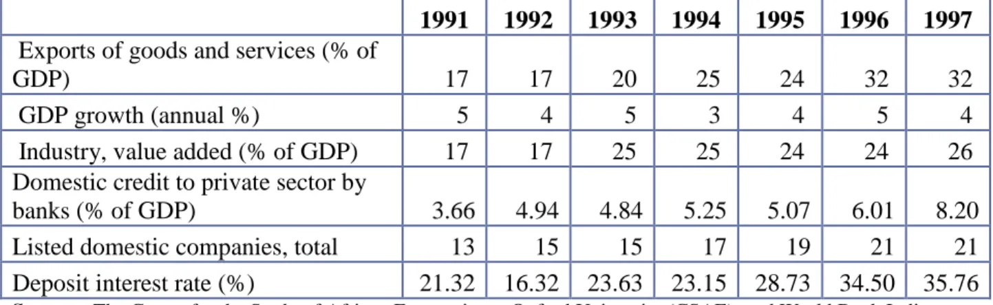
Table 2.1.1 – Ghana Macroeconomics Statistics ...70

Table 2.1.2 – Sample Sizes ...70

Table 2.2 – Definitions of Regression Variables ...71

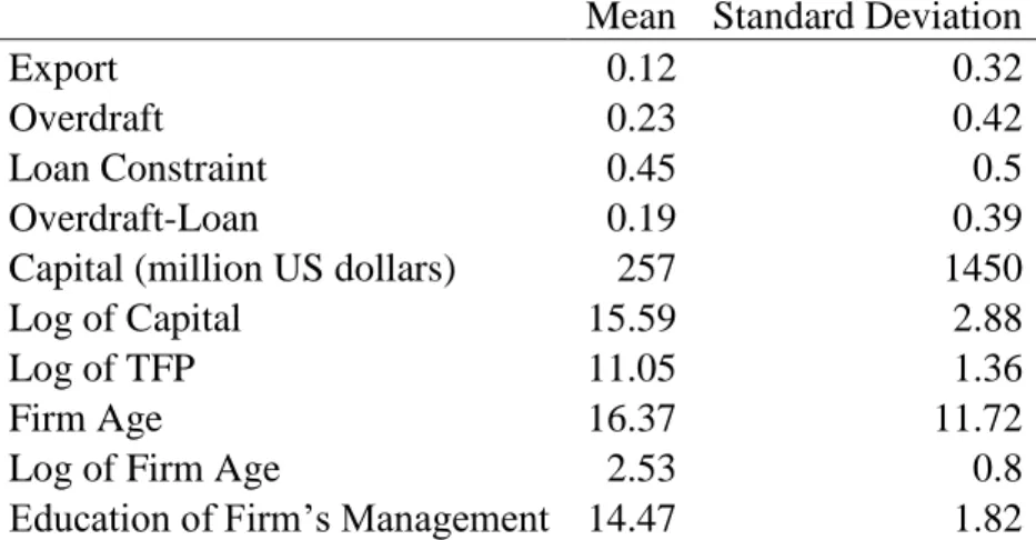
Table 2.3 – Descriptive Statistics for Key Variables (1991-1997) ...72

Table 2.4.1 – Correlation of Key Variables ...73

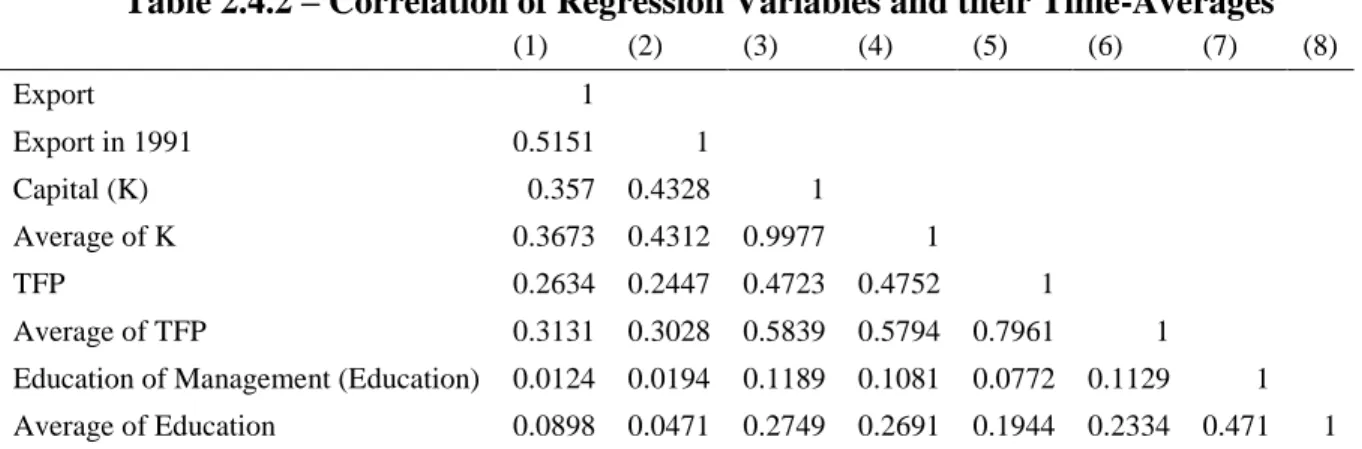
Table 2.4.2 – Correlation of Regression Variables and their Time-Averages ...73

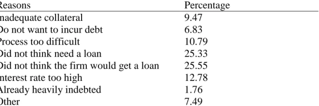
Table 2.5 – Reasons for Not Applying for a Loan ...74

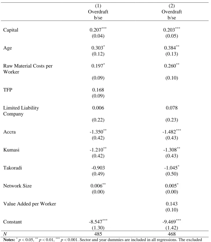
Table 2.6.1 – Determinants of Access to Overdraft...75

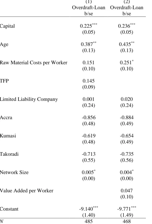
Table 2.6.2 – Determinants of Access to Both Overdraft and Loan ...76

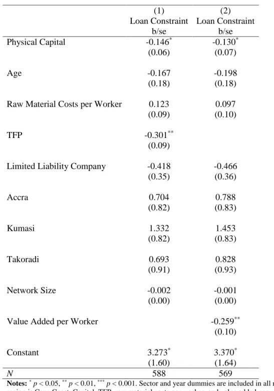
Table 2.7 – Determinants of Loan Constraint ...77

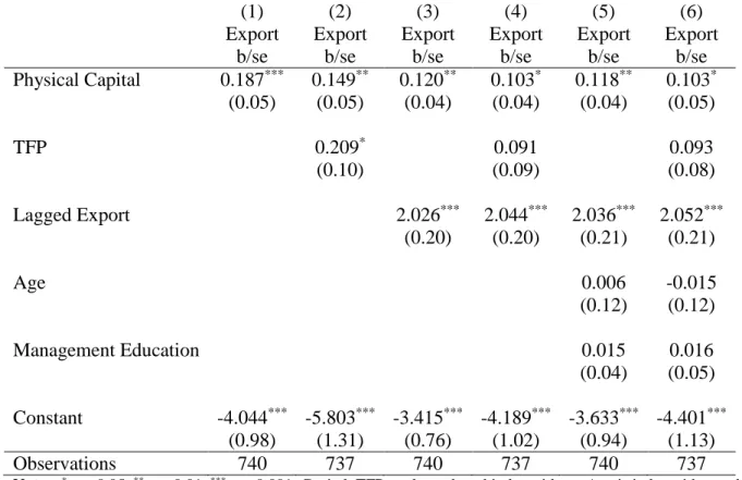
Table 2.8 – Regression of Export Status without Credit Access Variables (Pooled Probit) ...78

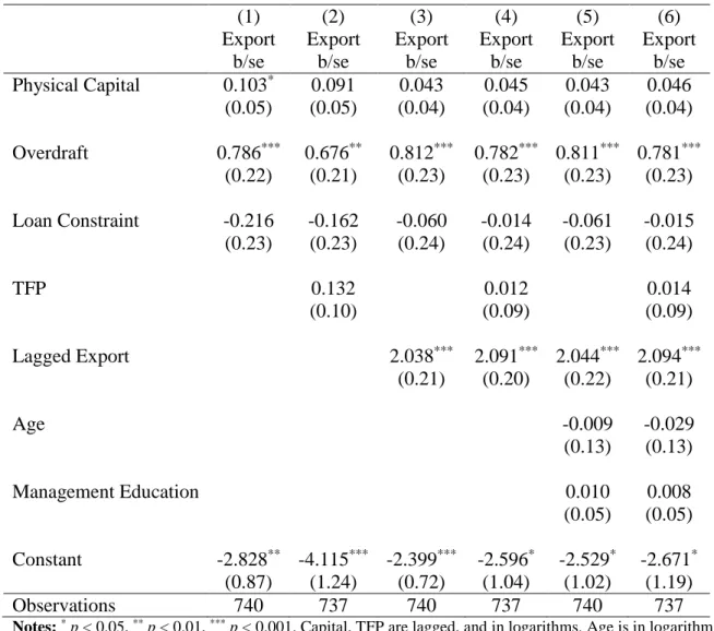
Table 2.9 – Regression of Export Status with Overdraft and Loan Constraint Indicators – Pooled Probit Estimation ...79

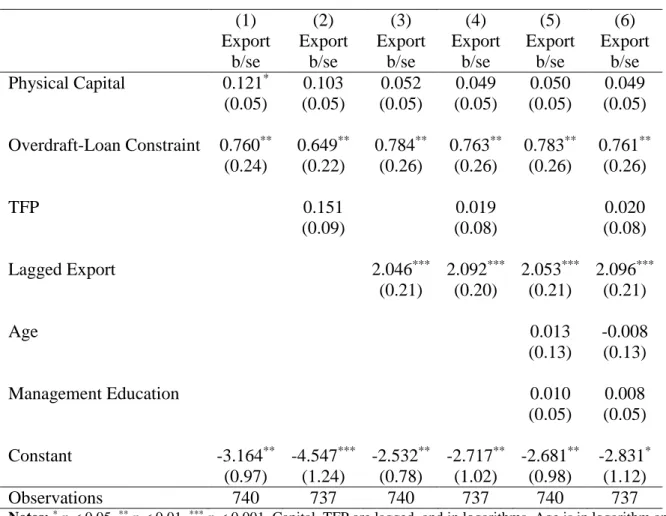
Table 2.10 – Regression of Export Status with Overdraft-Loan Constraint Indicator – Pooled Probit Estimation ...80

Table 2.11 – Regression of Export Status with Lag of Average of Loan Constraint – Pooled Probit Estimation ...81

and Loan Constraint Indicator ...82

Table 2.13 – Estimation of the Dynamic Probit with Overdraft-Loan Constraint Indicator ...83

Table 2.14 – Heterogeneous Effects of Access to Credit ...84

Table 2.15 – Checking Reverse Causation from Lagged Export status to TFP ...85

Table 2.16 – Checking Reverse Causation from Lagged Export status to TFP (Continued) – Regression of TFP according to fitted evolution equation of TFP ...86

Table 2.17 – Propensity Score Matching (Controlling for Lagged Export Status) – Treatment is Access to Overdraft in 1995 ...87

Table 2.18.1 – Checking Whether Credit Constraint Affects TFP – Regression of TFP According to a Fitted Evolution Equation of TFP where Credit Access is Included in the Motion equation for TFP ...88

Table 2.18.2 – Correlation between TFP Estimates ...88

Table 2.19 – Average Partial Effects (APEs) for the Dynamic Probit Regression of Export Status...89

Table 3.1.1 – Some Macroeconomic and Credit Indicators for the Vietnamese Economy during 2005-2008 ...147

Table 3.1.2 – Innovation Activities of Enterprises ...148

Table 3.1.3 – Number of Enterprises by Province ...148

Table 3.1.4 – Most Important Constraint to Firm Growth ...149

Table 3.2.1 – Summary Statistics (2005-2008) ...150

Table 3.2.3 – Interest Rate of the Current Most Important Formal Loan ...151

Table 3.2.4 – Regression of the Interest Rate of the Current Most Important

Formal Loan ...152

Table 3.3 – Fixed Effect Estimation of the Baseline Regression ...153

Table 3.4.1 – Endogenous Switching Regression – Switching Variable is

Credit Constraint Indicator ...154

Table 3.4.2 – Endogenous Switching Regression – Switching Variable is Credit Constraint Indicator When Varying the Percentile Cutoff of Interest

Payment per Worker ...155

Table 3.4.3 – Endogenous Switching Regression – Switching Variable is the

Innovation Indicator ...156

Table 3.5 – Regression of Interest Payment per Worker against Lag of Log of

Revenue per Worker or Against Lag of Log of Gross Profits per Worker ...158

Table 3.6 – Matching Covariates for Matching when the Treatment is the

Credit Constraint Indicator ...159

Table 3.7 – Logistic Regression Results for the Propensity Scores ...161

LIST OF FIGURES

Figure 2.1 – Exporting Decision as a Function of Firm’s Productivity and Liquidity ...90

Figure 3.1 – Histogram of the Change in the Nominal Interest Rate of the

CHAPTER 1

Introduction

Exporting and innovation are two activities that receive great interest from policy makers in developing countries since they are often associated with reallocation of market share to the most productive firms, as well as with increases in economic growth and aggregate productivity. While real factors such as firms’ efficiency and innovative capacities are important in

determining exporting and innovation, lack of access to financing also has the potential to be an important obstacle to these activities.

Firms’ exporting and innovation activities tend to be more dependent on external financing than their other activities. Exporters incur higher fixed costs such as advertising and the costs of setting up foreign distribution networks. They also have larger needs for working capital since cross-border shipping takes a longer time, so exporters must fund their operating costs while awaiting payments from abroad. Projects involving innovation are riskier, more expensive, and take a longer time to complete than non-innovative projects.

Motivated by the fact that exporting and innovation are potentially more vulnerable to credit constraint, I look at the impact of credit constraint on these activities at the firm level. The dissertation contains two self-contained essays with the general theme of examining the effects of credit constraint on firms’ activities. The first essay looks at the impact of credit constraint on manufacturing firms’ export decisions in Ghana. The second essay looks at the impact of credit constraint for innovating firms in Vietnam, focusing on distinguishing whether innovating firms face a tighter credit constraint. Both essays extend the Melitz (2003) model of firms

heterogeneous in productivity by incorporating the borrowing and lending decisions, and, in the second essay, by examining the innovation decision in addition to the export decision.

In the first essay, I build a theoretical model of firms heterogeneous in productivity, internal funds, and collateral capacity that is an extension of the Melitz (2003) model of firms

heterogeneous in productivity. The theoretical model predicts that a firm’s access to credit has a positive effect on its decision to export. This positive effect of access to credit on export

propensity is most pronounced for firms in the intermediate range of productivity levels. To test the theoretical predictions, I examine the effect of access to bank credits on firms’ export

as capital, age, and education of the firm’s management, access to a bank overdraft facility increases a firm’s likelihood to export by 7.6 percentage points. There is also empirical evidence that suggests access to credit matters most for the exporting decisions of firms in the

intermediate range of productivity.

In the second essay, I build a model of firms heterogeneous in productivity that incorporate innovation decisions. Because of asymmetric information, banks cannot observe firms’

productivity levels. This causes banks to impose a credit constraint by lending to the firms less than the amount the firms need, to ensure that the firms have an incentive to reveal their true productivity when applying for loans. As a result, there is a gap between the firm’s actual output level and its first-best level. Innovation results in higher productivity if successful, but involves higher risks and a longer time to complete. For this reason, banks impose an even tighter credit constraint on innovating firms and thus, innovating firms have an even wider gap between their first-best output levels and their actual output level. These predicted relationships are represented in an estimating equation of the production function type, which is derived from the theoretical model. The estimating equation predicts a positive relationship between a firm’s interest

payment per worker and its revenue or profits per worker for non-innovating firms, and a similar positive relationship, though of smaller magnitude, for innovating firms. To address the

endogeneity of the interest payment per worker and innovation, I also estimate an endogenous switching regression where the endogenous switching variable is the credit constraint or innovation indicator, and conduct matching with the treatment being the credit constraint indicator. Overall, the empirical estimation results support the theoretical predictions that credit constraint has a negative impact on firms’ revenue (profits) and this effect is higher for

In conclusion, the two essays show the negative impacts of credit constraint on exporting and innovating for two less-studied countries, Ghana and Vietnam, and, in the second essay, a population of firms that is less studied, small and enterprises (SMEs). Ghana and Vietnam are two examples of developing countries that have undergone trade liberalization and some reforms of the financial system. However, despite the fact that the economies in these two countries were open during the period investigated by this chapter, their financial systems were still

CHAPTER 2

Exporting and Firm-Level Credit Constraints – Evidence from Ghana

I. Introduction

For many developing countries where the financial system is not very advanced, access to financing can be an important hindrance to firm growth and investment. For example, Bartlett and Bukvic (2001) found that the key barriers to the growth of small and medium enterprises (SMEs) in Indonesia were institutional environment characteristics such as bureaucracy and external financial constraints. The difficulty in access to financing is worsened by the fact that many firms in developing countries are small and need to rely on external financing to cover production costs. With evidence of significant fixed costs of entry into exporting documented in the trade literature (Roberts and Tybout 1997, Bernard and Jensen 2004, Girma et al. 2004, Nguyen and Ohta 2007), this raises the question of what role financial constraint has in the decision to export by a firm in a developing country. This study answers the question by analyzing the impact of financial constraints on firms’ decisions to export in Ghana.

The impact of firm-level financial constraints has been studied by many scholars. However, most studies focus on the impact of financial constraint on firm growth and/or the firm’s

Studying the impact of credit constraint on exports is important because compared to

domestic production, exporting requires additional financing. For example, exporters may incur fixed costs of learning about foreign markets, advertising, and setting up a distribution network in the foreign markets. Exporters also have to cover additional variable costs associated with exporting, such as duties, shipping, and freight insurance. Because of cross-border, long-distance shipping, the delay for exporters to receive order payments tends to be longer than for domestic producers. This implies that exporters have higher working capital requirements than domestic producers. Lenders may be more reluctant to finance exporting, since information about foreign markets and potential profitability is more difficult to obtain than for domestic sales. Payment enforcement is also more difficult in a foreign country, so exporters may face a higher risk of late payment or non-payment from clients.1

This chapter explains the link between a firm’s credit access and its export participation. In doing so, this chapter highlights the importance of credit access in firm exporting decisions and the interaction between credit access and firm productivity in determining a firm’s export status. The chapter includes a theoretical model that links financial and export decisions, and empirical testing of the model. Similar to previous literature on exporting from the new trade theory, my model recognizes the role of firm productivity and fixed costs of export. The theoretical contribution of this chapter is that it models explicitly how firms can cover their costs of exporting through borrowing, incorporates endogenous loan default, and models the banks’ lending decisions that are based on their assessment of the firm’s characteristics and collateral.

1_{A more detailed list of the various reasons why exporting requires additional external financing compared to}

My theoretical model builds on Melitz (2003) and Chaney (2005). I assume that firms face difficulty in overcoming financial constraints in exporting but not in producing for the domestic market.2 The assumption is reasonable since exporting involves more uncertainty, which reduces the willingness of investors to lend money for exporting. I also assume that firms draw

exogenous liquidity shocks. Since my focus is on firm-level financial constraints, I abstain from analyzing financing differences across sectors and countries as in the approach in Manova (2008) and in Muûls (2008). I extend Chaney’s model (2005) by allowing firms with liquidity shortage to borrow from banks to cover fixed costs of exporting. More importantly, the main difference between my model and those of Chaney (2005), Muûls (2008), and Suwantaradon (2008) is that I model explicitly the firm’s borrowing decision and the bank’s lending decision under imperfect information as well as endogenous bankruptcy caused by a combination of firm-level shocks in export income and the bank’s lending decisions based on firm characteristics.3

My model predicts that a firm’s credit constraint has a negative impact on its export

propensity, especially if the firm is in the intermediate productivity range. The empirical section of this chapter distinguishes between two types of external financing: (1) the financing for working capital and unexpected liquidity shortage with bank overdraft facilities and (2) the financing of investments and longer-term costs with bank loans. The results of the empirical estimation suggest that having access to overdraft facilities increases a firm’s likelihood to

2 _{Both Chaney (2005) and my model assumes that firms can borrow to cover fixed costs of production for domestic}

market at zero interest rates.

3 _{Chaney (2005) does not model external financing. In Manova (2008) and Muûls (2008), firms are assumed to}

export, but access to loans does not significantly affect a firm’s export propensity. Furthermore, the empirical results also confirm the heterogeneous effect of access to credit: the positive effect of access to overdraft on export likelihood is only present for firms in the intermediate range of productivity.

II.Literature Review

The literature relevant to this chapter comes from two branches: the literature on exporting by heterogeneous firms with costs of entry into the export markets, and the literature on the effect of firm’s financial constraint on firm’s investment and export decisions. Throughout this chapter, the term “sunk export (entry) costs” refers to a one-time fixed cost of entry that firms need to pay to start exporting. This fixed cost of entry into exporting will become sunk once it is paid.

Similarly, the term “sunk costs of operation” or “sunk costs of beginning production” refers to a one-time fixed cost that the firm has to pay in order to begin operation; this entry cost will become sunk once it is paid.

firms. Positive effects of productivity on a firm’s probability to export were found in Colombia and Morocco (Clerides et al. 1998), and in nine sub-Saharan African countries during the period 1992-1996 (Van Biesebroeck 2005). On the other hand, no self-selection effect into exporting was found for the UK manufacturing sector in the period 1989-2002 (Girma et al. 2004), in Indonesia during the period 1990-1996 (Blalock and Gertler 2004) or in Mexico during 1986-1990 (Clerides et al. 1998). Bernard and Jensen (2004) find that firm heterogeneity is substantial and important in the export decision: firms that have larger size, higher labor quality, or product innovation are more likely to self-select to become exporters. However, firm productivity is found to have no significant effect on the probability of exporting in the specification preferred by the authors. Rankin (2005) investigated firms’ export decisions using panel data of

manufacturing firms in five African countries (Kenya, Ghana, Tanzania, South Africa, and Nigeria). He finds that firm size is a robust determinant for the firm’s export participation decision, but productivity is not. Nguyen and Ohta (2007) also find productivity to be insignificant in determining export propensity.

self-selection across a large number of countries and industries, but concludes that there is not necessarily a learning-by-exporting effect.

In addition to firm heterogeneity, other authors have focused on the role of sunk entry costs in exporting. Most studies confirm that there are significant sunk costs associated with entry into exporting. Roberts and Tybout (1997) model how firm (profit) heterogeneity and sunk costs of entry into the export market affect firms’ decision to export. Based on this theoretical model, a dynamic probit regression is run with the dependent variable being the firm’s current export status and the independent variables being the firm’s export participation in previous years and firm characteristics. They find a significant effect of sunk entry costs with prior export

experience being estimated to increase the probability of exporting by as much as 60 percentage points. Bernard and Jensen (2004) find that exporting today raises the probability of exporting tomorrow by 39 percent for U.S. manufacturing firms. Girma et al. (2004), and Nguyen and Ohta (2007) find past export participation to be positively correlated with export propensity for the U.K. manufacturing sector in the period between 1989 and 2002 and for Vietnamese firms in the period of 2002-2004.

While the majority of studies on firm financial constraints have focused on the impact of financial constraint on firms’ growth, investment, and/or innovation decisions, some recent studies have begun to examine the role of financial constraint on firms’ exports. Garcia-Vega and Guariglia (2012) extend the Melitz (2003) model by incorporating a new dimension of firm heterogeneity: random income volatility, [0,).4 Their model predicts that it is more costly for more volatile firms to obtain external financing from banks. Also, assuming that demand shocks in the national and international markets are negatively correlated and the fixed costs of exporting are not too high, firms with higher national income volatility are more likely to export than those with low national income volatility because trade helps these firms to reduce their probabilities of bankruptcy.

Pratap and Urrutia (2004) study the balance sheet effects of the 1994 Mexican crisis. They build a dynamic model where firms are heterogeneous in productivity, capital stock, and level of foreign debts, and firm productivity follows a first-order Markov process. The authors impose financial market imperfections by assuming that firm investment can only be financed with internal funds or from the international financial market. As a result, their model predicts a positive correlation between foreign debts and exports, and between capital and exports. Using panel data of Mexican firms, Pratap and Urrutia observe that large firms get larger loan amounts at lower interest rates prior to the credit crisis. They also observe that the loan interest rate is an increasing function of the size of the loan.

4 _{Specifically, a firm’s income in period t is given by z(}_)p(_)y(₎

On the theoretical side, Chaney (2005) is the closest to my model. Chaney extends the Melitz framework by incorporating randomly drawn liquidity shocks. Under these assumptions,

compared to Melitz (2003), the most productive firms are further partitioned into the most productive firms that can export because they generate enough liquidity from domestic sales to overcome liquidity constraints, and the less productive firms that would find it profitable to export but cannot because of liquidity constraints. This prediction is in line with the empirical facts that few firms export, and that exporters are typically not liquidity constrained. Chaney’s model also predicts that the scarcer the available liquidity and the more unequal the distribution of liquidity among firms, the lower are total exports. It should be noted that there is no

borrowing channel in the Chaney model, where firms can finance (fixed) costs of exporting with only their internal funds, while my model allows for borrowing from banks.

development, and in more financially vulnerable sectors. Manova (2013) tests her predictions with unidirectional bilateral exports for 107 countries and 27 sectors over the 1985-1995 period and concludes that the regression results support her hypotheses.5

Muûls (2008) seeks to analyze whether there is any interaction between firm-level constraints and exporting. Her model combines the Chaney (2005) model and the external financing element from Manova (2008). Specifically, firms have three sources of liquidity to finance the fixed costs of exporting: internal financing and exogenous random liquidity shocks as in Chaney (2005) as well as external financing as in Manova (2008).6 Muûls’ predictions are a hybrid between those of Chaney (2005) and Manova (2008). In particular, her model predicts that (1) there are firms that would find exporting profitable but are prevented from exporting because of credit

constraints, (2) more productive and less credit-constrained firms will export to more destinations and to relatively smaller markets, and (3) an appreciation of the exchange rate between the domestic and the foreign currencies has three effects: (a) existing exporters become less competitive and reduce their exports, (b) the least productive existing exporters stop

exporting, and (c) the most productive constrained non-exporters start exporting. Muûls then tests her model’s predictions with a data set of Belgian manufacturing firms. She uses the Coface

5 _{Her main measure of a country’s financial development is the amount of credit by banks and other financial}

intermediaries to the private sectors as a share of GDP. Other measurements of financial development that are used for robustness checks are repudiation of contracts, accounting standards, and risk of expropriation. A sector’s need for external finance is the share of capital expenditures not financed with cash flow from operations for the median firm in each industry. A sector’s asset tangibility is defined as the share of net property, plant and equipment in total book-value assets for the median firm in the sector. These industry measures are constructed from U.S. data.

6 _{As in Chaney (2005), Muûls assumes that there is no liquidity constraint for firms to finance their domestic}

production. It is also assumed that firms can finance the variable costs of exporting internally. External financing is modeled as in Manova (2008). The external credit constraints are modeled with two parameters: ts, the proportion of

score as a measure of credit constraints.7 Her empirical results confirm the model’s second and third predictions. However, for the regression of the propensity of becoming a new exporter that is used to test the first prediction, although the impact of firm productivity (log TFP) and firm size (log employment) are found to be significantly positive, credit constraint is found to have an insignificant impact on firms’ export propensity.

Suwantaradon (2008) also assumes heterogeneous firms (with a random draw of

productivity), but assumes a different production function where capital is the only input.8 A firm finances capital with its own net worth and one-period debt. Firms, however, can only borrow up to a fixed multiple of their net worth. This fixed multiple is identical across firms and is

interpreted as representing the degree of financial frictions in an economy. With this assumption, the borrowing constraint that firms face depends only on net worth and not on other factors such as firm productivity. Suwantaradon’s model predicts that under financial constraints, even among a group of firms with the same productivity level, firms that are more financially

constrained operate on a less efficient scale and, as a result, may no longer find operating and/or exporting profitable. Furthermore, financial frictions can have persistent impacts on firms’ dynamics. Productive firms with very low starting net worth will never accumulate enough to

7 _{According to Muûls, Coface International is a credit insurance company that provides credit information and}

insurance services. The company manages an international buyer’s risk database on 44 million companies. The Coface score is constructed by Coface International as a bankruptcy measure. The Coface score ranges from 3/20 to 19/20. Coface International separates firms into three categories based on their scores: “maximum mistrust” (3 to 6/20), “temporary vulnerable” (7 to 9/20) and “normal to strong confidence” (10 to 19/20)

8 _{The production function is as follows: for a domestic firm,}





t t

t z Max k f

y   ; for an exporter,





t

t z Max k f f

y    where y_t, z_t, k_t, fdand f xare firm’s output, productivity, capital, fixed costs of domestic production and fixed costs of exporting respectively. Capital stock is determined as: k_t i_tb_t

overcome credit constraints and therefore, will never start operating and exporting even if they are very productive.

Regarding the empirical literature about the impact of credit (financial) constraint on firms’ exports, Campa and Shaver (2002) uses a panel of Spanish manufacturing firms in the 1990s to test the effects of firm financial constraints on export status. They find that exporters face less severe liquidity constraints and have more stable cash flows than non-exporters. They interpret this as evidence for causality from export status to liquidity constraint as foreign sales help firms relax the liquidity constraint. It should be noted that Chaney (2005) argues that since Campa and Shaver find that export intensity does not matter for liquidity constraint, their empirical results actually point to the causality direction from liquidity constraint to export.

Correa et al. (2007) find that having loans increased Ecuadorian firms’ exports. However, this result should be taken with caution since Correa et al. do not control for the role of sunk entry costs in exporting. Zia (2008) uses a different approach to identify the impact of firm-level financial constraint: the natural experiment approach. She studies the impact of the Pakistani government’s removal of subsidized export loans. Zia finds that after the policy change,

privately owned firms experience a significant decline in their exports, while large and publicly listed firms were unaffected. There was no evidence that less productive firms are more affected by the removal of loan subsidies. On the other hand, large firms, firms in corporate networks, or firms that have relationship with multiple banks are better in overcoming their financial

constraints.

In the macroeconomics literature, there is a large literature on the impact of liquidity

equilibrium real business cycle model to explain sudden stops in emerging countries following a severe financial crisis. Gertler et al. (2007) find that financial frictions explain half the decline in economic activities in Korea during the financial crisis of 1997-1998.

Since the empirical part of this chapter uses proxies for firm-level credit constraint, I would like to mention measures of firm-level constraints that have been used in the literature. These measures can be grouped as follows. First, there is a large literature started by Fazzari et al. (1988), that identifies financially constrained firms by testing whether, after controlling for other variables, financial variables that capture the availability of internal sources of finance and the net-worth position of firms, such as cash flows, would have a significant effect on investment decisions for firms that are thought (a priori) more likely to face information and incentive problems. The theoretical rationale behind these analyses is that firms that suffer from more asymmetric information problems are more sensitive to variations in their net worth or changes in the availability of internal funds. This approach often faces a critique that the financial variables may capture the effect of unobserved investment opportunities instead of financial constraint. The second approach is to use financial variables from firms’ balance sheets (such as cash flow, leverage ratio, liquidity ratio, etc.) to proxy for financial (credit) constraint. The third approach is to use indicators that capture access to loan, etc. as proxies for firms’ credit

constraint. The fourth approach is to use a firm’s subjective report of considering credit access as one of the biggest obstacles. In this chapter, I will use the third approach, but instead of looking just at access to bank loans, I will also look at access to overdraft facilities.9

9 _{The data set of Ghanaian firms that I use in the empirical estimation has many missing values in investment, and}

III. Theoretical Model

My model shares several similarities with the models in Melitz (2003) and Chaney (2005): constant elasticity of substitution (C.E.S) preference, firms that are heterogeneous in

productivity, and a market equilibrium characterized by the zero-profit condition and the free-entry condition. However, in my model, firms are also heterogeneous in two other dimensions, their liquidity and collateral. Thus, while the segmentation of firms into non-producer, domestic producers, and exporters in Melitz’s model is only based on productivity, the segmentation of firms in my model is not only based on productivity but also on firm’s liquidity and collateral. In addition, I also introduce an exogenous income shock to exporters, which can be caused by a shock to the demand for the exported variety, a feature that is borrowed from Garcia-Vega et al. (2012).10 _{This shock allows me to achieve a more realistic equilibrium where because of the} uncertainty at the lending time, banks still lend to some firms that end up going bankrupt.

1. Consumers (Demand)

There are two symmetric countries. In each country, the preferences of a representative consumer are given by the following intertemporal utility function:







 

0

0 log )

(x Y e dt

U_{t t t} t

where is the discount factor, x0 is the consumption of a numeraire good, and Y _t is an index of

consumption of the differentiated products that reflects consumers’ taste for varieties in period t.

10 _{Garcia-Vega et al. (2012) assume that the standard deviation of the shocks varies across firms and such, represent}

  1/ 0

,    

    Mt

t z

t y dz

Y

with 0 < ρ <1, yz,t is the quantity of variety z of the differentiated product demanded by

consumers in period t, Mt is the mass of firms in the stationary competitive equilibrium,

and1/(1) is the elasticity of substitution among varieties.

The aggregate price index for the differentiated product is a weighted price index of the prices of each individual varietyp_z,t:

) 1 /( 1

0 1

, ,

 

 

    

  





P

t

M t z t

Y

The aggregate expenditure, R_t, is normalized to one, and the demand for variety z in period t can be expressed as follows:

 

 

 ₁

, , ,

t Y

t z t z

P p

y (2.1)

2. Firms

For simplification of notation, I omit the firm and time subscripts (i and t) in this section. In terms of notation, the superscripts D and X refers to the domestic market and the foreign market respectively.

2.1. Firm production

In each country (home or foreign), there is a continuum of firms. There are three sources of heterogeneity among firms: (1) their level of productivity φ, (2) exogenous liquidity

and k(A) are density functions for productivity, liquidity endowment, and collateral respectively, and F(φ), G(n) and K(A) are the respective cumulative distribution function, hereafter referred to as c.d.f. All of the three distributions are known to both firms and banks.

Both domestic and exporting firms are hit by exogenous death shocks with probability p every period. In each period t, if firm i decides to export, it will face an export income shock zit

(domestic production involves no income shocks). The income shock follows a normal distribution N(1,2) which is left-truncated at zero. In other words, the distribution of the income shock is common across firms and across time periods. This distribution is known to everyone in the economy, including the firms and banks. The export income shock can be thought of as a shock to the price of the exported goods caused by a reduction in foreign demand for those goods. When the firm makes its export decision in period t, it knows its productivity shock for that period but it does not know the export income shock for that period yet. To operate, potential entrants have to pay a sunk entry cost feto start operation. If a firm wants to enter the export market, it has to pay a sunk entry costs in exporting fex to start exporting.

The firm production function is as in Melitz (2003):

  

) ( )

(

D D

D y

f

l  

  

) ( )

(

X X

X y

f

l  

equivalent to having lower marginal costs. To produce the same amount of output (y), a more productive firm will need less labor than a less productive one.

As common in the literature, exporting is assumed to be subject to iceberg transportation costs such that for each  units of the goods that are shipped abroad, only 1 unit arrives. Profit

maximization leads to the following pricing rules that equate marginal revenue and marginal cost in the domestic and in the foreign markets:

  ) ( D

p

  ) (

X p

where  is the common real wage rate in the home country. The optimal pricing rule implies that more productive firms charge a lower price both domestically and abroad since they have lower marginal costs.

Revenue from selling in domestic market and from exporting for a firm with productivity  is:

1 1

) ( )

(   

 _  _ 

P P

R rD

D μ X

r τ

r  1

2.2. Firms’ Decisions

Firms can borrow at zero interest rate to cover the fixed costs of production for the domestic market (f D). However, if they want to export and their liquidity is lower thanf X, they face a cash-in-advance constraint for exporting in each period. If these firms decide to export, they have to borrow from banks a loan equal to the fixed costs of exporting (f X ) at an interest rate r

where r > r0, the interest rate on riskless assets.11 To make the analysis simple, I assume that the

liquidity of a firm is fixed, i.e. firms cannot add their profits to the stock of liquidity but just distribute all the profits as dividend payments. At the end of the period, if paying back the loan makes the firm’s net worth negative, the firm defaults, exits, and the bank gets the firm’s net worth and collateral at that time. Otherwise, the firm will pay back the original loan amount plus interest.

Profits from selling in the domestic market, hereafter called domestic profits, are:12

D D D D D D D D D D f r f y y p            

  ( ) ( , ) * ( , )  ( , ) (2.2)

where 1/(1), rD(,D) is domestic revenue, and Dis the productivity cutoff that solves D 0. It can easily be seen that domestic profit is increasing in productivity. This

11 _{Since lending to exporting firms involve a risk that some firms may default, the interest rate that banks charge on}

these loans are higher than the interest rate on riskless assets.

12 _{The firm’s income from domestic production is:}

n r f r n r f y y p I D D D D D D D D D D ) 1 ( ) , ( ) 1 ( ) , ( * ) , ( )

(     ₀     ₀

            

implies that every firm that has a productivity draw less than the cutoff Dwill exit the market immediately while every firm with productivity above this cutoff will produce (at least) for the domestic market.

Let  X,NB be the productivity cutoff that solves:

0 ) 1 ( ) , ( ) 1 ( ) , ( * ) , ( ) , ( ) ( 0 , 0 ,         X NB X X X X X X X X NB X f r r f r y y p E               (2.3)

where E is the expectation operator.13 _{As is common practice in the trade literature, I assume the} fixed costs and iceberg transportation costs are such that D X,NB.14 _{Under this assumption,} firms with  D  X,NB will produce only for domestic market regardless of the level of their liquidity n and collateral A. These are unconstrained domestic producers because they would not export even if the loan for export has zero interest rate.

Firms with n ≥f Xand X,NBwill find it profitable to use their own liquidity to finance fixed costs of export.15 _{They also earn the riskless interest rate on the remaining liquidity after} paying for the fixed costs of exports. Thus, their income in period t is:

13 _{Again, this cutoff is deduced by equating the firm’s expected income for non-borrowing exporting with its outside}

opportunity of producing for only the domestic market.

14 _{Specifically, as shown in Melitz (2003),} X,NB_> D _{if and only if} 1_f x _f D

15 _{The costs of using firm’s own liquidity to cover fixed costs is the forgone interest earned at the riskless interest}

rate r0 while the costs of borrowing from banks are the interest payments at the loan interest rate r > r0. Therefore,

) )( 1 ( ) , ( * ) , ( ) , ( ₀ , X X X X X X it D NB X f n r y y p z I                 (2.4)

The probability that a non-borrowing exporter does not survive the export income shock is:

                       _{   }                 ) , ( ) , ( 1 ) )( 1 ( / ) , ( * ) , ( ) , ( ) )( 1 ( / ) , ( * y Probabilit 0 ) )( 1 ( ) , ( * ) , ( ) , ( y Probabilit 0 0 0 , X X X D X X X X X X D X X X it X X X X X X it D NB X y p f n r y y p f n r y z f n r y y p z                                (2.5)

where  is the c.d.f of the standard normal distribution that is left truncated at 1/ (since z_it

follows a truncated normal distributionN(1,2) which is left truncated at zero).

Firms with n <f X that find borrowing for exporting profitable will borrow to export. If they obtain a loan from the bank at the loan interest rate r, their income would be:

n r f r y y p z I X X X X X X it D B X ) 1 ( ) 1 ( ) , ( * ) , ( ) , ( ₀ , _{    }  _{ }         

Let  X,B be the productivity cutoff that solves

0 ) 1 ( ) ( ) 1 ( ) ( * ) ( ) ( )

( ,        X 

X X X X X B X f r r f r y y p E           (2.6)

Firms with n < X

f

 and  X,B

will produce only for the domestic market. Note that

NB X B X,  ,

to export. Also, note that the cutoff X,Bis a function of the loan interest rate that the bank charges to a firm.

Next, I solve for the export decision for firms with X,Band nf X. These are the firms that have an incentive to export but will have to decide whether to borrow for export. Suppose that the bank offers firms a fixed loan amount equal to f X at interest rates that differ across the firms, depending on the bank’s evaluation of the firm’s probability of defaulting on loan. In period t, for a firm i that gets a loan from the bank at an interest rate r_it, the probability of default is: B X X X D X X X X D X X it X B X X X X X it D D it it B X D it y p y n r f r y p y n r f r z P n r f r y y p z P n r , 0 0 0 , , 1 ) / * ( ) 1 ( ) 1 ( ) / * ( ) 1 ( ) 1 ( 0 ) 1 ( ) 1 ( ) , ( * ) , ( ) , ( ) , ( ) , , , , (                                                                     (2.7)

where again, denotes the c.d.f of a standard normal distribution left-truncated at 1/ . It can be shown that the probability of default is decreasing in firm liquidity and under certain

conditions, decreasing in firm productivity.16

Firms with  X,B and nf X will decide to export in period t if the expected discounted profit from borrowing to export, VX,B, is greater than or equal to the expected discounted profit from producing domestically, VD_{. Since the liquidity endowment, productivity and market}

structure do not change over time, a firm that decides to borrow to export in period t will still decide to borrow to export in the following periods given that it survives the exogenous death shock and has not defaulted on a loan. Similarly, a firm that decides to produce only

domestically in period t will continue to produce only for the domestic market in the following periods given that it has survived the exogenous death shock in previous periods.

Recall that  is the discount rate. Let VtXB

,

and VtDbe the firm’s expected value at time t of borrowing to export and of producing only for domestic market respectively. Then:

ex X it X X X D B X it B X

t r f r n f

y y p p r n

V _

              

 * (1 ) (1 )

) 1 )( 1 ( 1 1 ) , ,

( _{, 0}

,      





p n

VtD D (1 )

) 1 ( 1 1 ) ,

(   0

 

 

 

where fexis the sunk cost of entry into the foreign market and

D D D D D D D f y y p           ( ) ( , ) * ( , ) 

It can be shown that when





, productivity is positively related to export

propensity (see Appendix C). Specifically, among firms with  X,B

and X

f

n , the more productive the firm is, the more likely it will borrow to export. It can also be shown that when





 

 X X

D y p n r ) 1 (  ₀   

with being the p.d.f of the truncated normal standard distribution which

is left-truncated at 1/ , a firm with higher liquidity level will more likely borrow to export.17

This is because a firm with a higher liquidity level can earn more from the interest rate payments to their liquidity and thus, more likely to avoid bankruptcy if it borrows to export.

Note that since D X,NB  X,B(r_it) for any positive loan interest rate r_it, the model implies that all exporters also produce for the domestic market.18

3. Bank’s Lending Decisions

I assume a competitive banking industry in which banks make zero profits. A representative bank offers a fixed loan amount, f X . The bank observes the firm’s liquidity level and collateral

but does not observe the firm’s productivity. However, the bank forms an evaluation of this productivity as a function of the firm’s characteristics:

) (Z f

B _



where Z is a vector of firm characteristics. Based on this evaluation, the bank expects the

probability of default for the firm to be X,B(B,n). To keep the model general, I do not specify the elements of Z in the model but in the empirical section, I will estimate the determinants of credit constraint (access).

For firm i in period t, let zitBDefault

,

be the cutoff export income shock such that a shock less than zitBDefault

,

will cause a borrowing exporter with productivity B and liquidity n to go bankrupt. Then z_itB,Default solves:

18 _{One objection can be that in reality, we may have a corner solution where some firms serve only the foreign}

0 ) 1 ( ) 1 ( * ) , , ( ₀

,        X 

it X X X it D B it B X f r n r y y p z n z I    

 (2.8)

Let BMin it

z ,

be the lowest export income shock below which the firm’s net worth becomes negative. Then zitBMin

, solves: 0 ) 1 ( * ) , , ( 0 ,       n r y y p z n z I X X X it D B it B X   

 (2.9)

Let E_t





collateral) in the next period if the firm suffers from a bad export income shock and has to default. This expectation is based on the bank’s prediction of firm’s productivityB

and the

firm’s liquidity stock n. Note that the firm’s liquidity is observable to the bank but the firm’s

productivity is not.





E Default B it Min B it z z X X X it D B B X

t (1 ) ( )

* ) , ( , , 0 ,



where l(z)is the density function of the export income shock assumed as above to follow a truncated normal distributionN(1,2)left-truncated at zero.

For firm i that comes to borrow for export in period t, the bank will choose a loan interest rate

ritsuch that its expected return from lending equals the expected returns if the firm had invested

in riskless assets:













B B X t B B X X it B B X X A default n I E n f r n f

r     

 ) 1 ( , )(1 ) ( , ) ( , )

1

The left-hand-side (LHS) of the equation above is the return on riskless assets. The right-hand-side (RHS) consists of the expected repayments to the bank if the firm does not default (the first term on the RHS) and the expected collection the banks can make if the firm defaults (the second term on the RHS). E_t





productivity level and liquidity level.19 _{As shown earlier,} , _{( , )} n

B B X 

 is decreasing in both the firm’s liquidity level and the bank’s evaluation of the firm’s unobserved productivity. Therefore, it is obvious from the equation above that the bank’s loan interest rate to the firm is decreasing in the firm’s collateral value, in the firm’s liquidity level, and in the bank’s evaluation of the firm’s unobserved productivity.

As a summary, the segmentation of firms predicted by the model can be summarized in Figure 2.1, which is drawn holding collateral fixed. The graph holding liquidity fixed would be similar. Firms that have productivity less than the cutoff Ddo not operate at all (regardless of their liquidity and collateral) since they are not profitable. For firms that have sufficient liquidity (n) to finance the fixed costs of exporting, the productivity cutoff for exporting does not depend on liquidity n or collateral A. For these firms, the decision to export depends only on productivity and not on financial factors or collateral capability. For firms with insufficient liquidity, i.e., firms with nf X , the productivity cutoff for exporting depends on both the firm’s liquidity and collateral. Specifically, this cutoff is lower for firms with higher liquidity and/or collateral. In other words, for firms with insufficient liquidity, the importance of productivity on export decision is reduced as the export decision also depends on financial factors and collateral capability. The segmentation just described can be summarized in Figure 2.1. To achieve

analytical equilibrium solutions, I will assume that on average, the bank’s expectation of the probability that a firm defaults is correct, i.e. equal to the actual probability of default.

4. Aggregation

Denote M as the mass of firms in the equilibrium. Let MD be the number of firms in the home country that produce domestically only. Let MX,Bbe the number of borrowing exporters and MX,NBbe the number of non-borrowing exporters. As in the Melitz (2003) model, in equilibrium, the weighted average productivity of all firms in the home country (including both domestic and foreign firms) with the weight being the relative shares of firm outputs is:

1 1 1 , 1 , 1

, 1 , 1

] ) ~ ( )

~ ( )

~ ( [ 1

~      

   



 _{ }

 _  _{ }  _{ }  

 D D XB XB XNB X NB

M M

M

M (2.11)

Aggregate variables can be expressed as a function of this average productivity:

  

~ 1

) 1 /( 1 

M

P (2.12)

) ~ (

/ 1  

q M

Q

condition ensures that ex-ante expected profits from entering the market is driven down to zero since as long as expected profit is positive, more firms will enter which increases competition and drives the expected profits down until it comes to zero at which point a potential entrant is indifferent about entering the market. 20





Let D() be the equilibrium distribution of productivity levels for incumbent firms, i.e. firms that are productive enough to stay in the market, then D() is the conditional distribution of f()on [D,):

     _   otherwise 0 if ) ( 1 ) ( ) ( D D D F

f _{ }

    Similarly, ) ( 1 ) ( ) ( _, , NB X NB X F f     

 is the equilibrium distribution of productivity levels for

non-borrowing exporters, and





) , ( 1 ) ( ) ( _, , A n F f B X B X     

 is the equilibrium distribution of

productivity levels for borrowing exporters.

20 _{In the Firm’s Decision section, we can see that} X,B_{is a function of the bank’s loan interest rate, r}

it. On the other

hand, by assumption, rit is a function of firm collateral, liquidity andthe bank’s evaluation of the firm unobserved

productivity. Given our assumption that the expected value of the bank’s valuation of firm productivity is equal to the firm’s real productivity, X,B

     _{ }    otherwise 0 and if )] ( 1 )][ ( 1 [ ) ( ) ( , , X D X NB X NB

X n f

f G F

f _{  }

          _{ }   otherwise 0 and if ) ( ))] , ( ( 1 [ ) ( ) , , ( , , X D X B X B

X n f

f G A n F f A

n     

 



Using these conditional distributions, we can rewrite the three aggregate average productivities in terms of the corresponding productivity cutoffs as follows:21





1 1 ) ( ~   _        

D D D d





1 , 1 , ) ( ~ ,                

X NB _{n f}X XNB X NB d





A A f n n B X B X X ) ( ) ( ) , , ( ~ 1 1 , 1 0 0 , ,                _{   } 

Thus, the zero-profit conditions can be written as:22

) ~ , ( ) ~ (   

D D D

q f  ) ~ , ( ) ~ ( , ,    

XNB X XNB

q f



21 _{Note that the segmentation of firms into non-borrowing exporters and borrowing exporters not only depends on}

firm productivity but also depends on firm liquidity level. However, because I have assumed the distributions of liquidity and productivity are independent of one another, I can define the aggregate average productivity for domestic producers and for non-borrowing exporters independently of the liquidity level.

22 _{Since (1}_{r)nis the deposit and interest earnings on firm liquidity that the firm would earn regardless of}

) ~ , ( ) ~ ( , ,    

XB X XB

h f 

where q(D,~)[~/D]1 1, q(X,NB,~)[~/X,NB]11, and









h A XB

A f n n B X X ) ( ) ( ) , , ~ ( 1 )] , ( / ~ [ ) ~ ,

( , 1

0 0 ,      _    _{ }   

 

This implies that average aggregate profit can be expressed as:

) ~ ( ) ~ ( ) ~

( D X,NB X X,NB X,B X X,B D

p

p    

 

    (ZCP)

= f Dk(D,~) pX,NBf Xk(X,NB,~) pX,Bf Xh( X,B,~)

where pX,NB and pX,B are the ex-ante probability that an operating firm will export without borrowing, and the ex-ante probability that an operating firm will borrow to export, respectively. These probabilities are calculated as follows:















f G

p _AA _nf XB

D X B X X ) ( ) ( ) , ( 1 ) ( 1 ) ( 0 0 , ,      _ _   

where F and G are defined above as the cumulative distribution functions of productivity and liquidity. The ex-ante probability an entrant is a non-borrowing exporter (pX,NB) is the

probability that conditional on drawing a productivity level greater than the productivity cutoff for operating (D), an entrant draws a liquidity that is less than the fixed costs of exporting and has a combination of liquidity and collateral such that it is profitable to borrow to export. The ex-ante probability that one of the surviving firms will export is:

B X NB X X

p p

p  ,  ,

Let e denote the ex-ante net value of entry and  denote the average present value of operating firms. Free entry implies that potential entrants will enter the market as long as the expected net value of entry is positive. Therefore, in equilibrium, the ex-ante net value of entry is zero, hence called the free entry condition.

0 *

market) in the

stay enough to high

draw ty productivi a

get y(firms

Probabilit  

 e

e  f



or _e 





where





) 1 ( 1 ) 1 (

0 p _p

t

t

   





  



 , is the discount rate, feis the fixed cost of entry

which is sunk thereafter, and pis the probability firms will be hit by a death shock in each period. Thus, the free-entry condition can be rewritten as:





) ( 1

) 1 ( 1

D e

F f p   

  

 (FE)

The (ZCP) and (FE) conditions determine the productivity cutoffs. The mass of firms in equilibrium can be determined as:

) ~ ( ) ~

( 



 r

L r

R

where L is the country’s population. The mass of export firms is pXM .

The model yields two predictions. The first prediction implies that access to finance, on average, increases firms’ export propensity. This prediction is illustrated in Figure 2.1. For the group of firms that does not have enough internal funds to cover the fixed costs of exporting but is productive enough to be profitable from exporting, only some firms - those that have access to bank financing - can export. This implies that access to bank financing should have a positive effect on firms’ export status.

The second prediction is that the effect of access to credit on firms’ export propensity is heterogeneous: access to credit has the most positive effect on export propensity for firms that are in the intermediate range of productivity. For firms that have very low productivity levels, i.e., less thanX,NB, whether the firms have access to financing does not affect their export decisions. In addition, the model implies that the cutoff productivity for exporting for borrowing firms (X,B) is decreasing in productivity, illustrated in Figure 2.1 by the downward-sloping curve of  X,B. This means that firms that are very productive are much more likely to be profitable from exporting even when they have to borrow. For these reasons, access to credit does not have much effect on the export decisions of the least and most productive firms, but has most impact on the export decision of firms that are in the intermediate range of productivity. Intuitively, the most productive firms can generate enough internal funds from their domestic sales to cover most of the costs of exporting, so external financing is not as important for their export decision. The least productive firms would not export even when there is no credit

in the intermediate range of productivity. These firms have the potential to gain profits from exporting, but need external financing to export since they are not productive enough to generate sufficient internal funds to finance exporting. In the empirical estimation, I will test the two hypotheses above.

IV. Empirical Testing

1. Credit Constraints in Ghana