CRC Press Utility Based Learning from Data 2010 RETAiL EBook pdf

(1)

(2)

Utility-Based

Learning from Data

(3)

Chapman & Hall/CRC

Machine Learning & Pattern Recognition Series

SERIES EDITORS

Ralf Herbrich and Thore Graepel

Microsoft Research Ltd.

Cambridge, UK

AIMS AND SCOPE

This series reflects the latest advances and applications in machine learning

and pattern recognition through the publication of a broad range of reference

works, textbooks, and handbooks. The inclusion of concrete examples,

appli-cations, and methods is highly encouraged. The scope of the series includes,

but is not limited to, titles in the areas of machine learning, pattern

recogni-tion, computational intelligence, robotics, computational/statistical learning

theory, natural language processing, computer vision, game AI, game theory,

neural networks, computational neuroscience, and other relevant topics, such

as machine learning applied to bioinformatics or cognitive science, which

might be proposed by potential contributors.

PUBLISHED TITLES

MACHINE LEARNING: An Algorithmic Perspective

Stephen Marsland

HANDBOOK OF NATURAL LANGUAGE PROCESSING,

Second Edition

Nitin Indurkhya and Fred J. Damerau

UTILITY-BASED LEARNING FROM DATA

Craig Friedman and Sven Sandow

Chapman & Hall/CRC

Machine Learning & Pattern Recognition Series

Utility-Based

Learning from Data

Craig Friedman

Sven Sandow

(4)

Chapman & Hall/CRC

Machine Learning & Pattern Recognition Series

SERIES EDITORS

Ralf Herbrich and Thore Graepel

Microsoft Research Ltd.

Cambridge, UK

AIMS AND SCOPE

This series reflects the latest advances and applications in machine learning

and pattern recognition through the publication of a broad range of reference

works, textbooks, and handbooks. The inclusion of concrete examples,

appli-cations, and methods is highly encouraged. The scope of the series includes,

but is not limited to, titles in the areas of machine learning, pattern

recogni-tion, computational intelligence, robotics, computational/statistical learning

theory, natural language processing, computer vision, game AI, game theory,

neural networks, computational neuroscience, and other relevant topics, such

as machine learning applied to bioinformatics or cognitive science, which

might be proposed by potential contributors.

PUBLISHED TITLES

MACHINE LEARNING: An Algorithmic Perspective

Stephen Marsland

HANDBOOK OF NATURAL LANGUAGE PROCESSING,

Second Edition

Nitin Indurkhya and Fred J. Damerau

UTILITY-BASED LEARNING FROM DATA

Craig Friedman and Sven Sandow

Chapman & Hall/CRC

Machine Learning & Pattern Recognition Series

Utility-Based

Learning from Data

Craig Friedman

Sven Sandow

(5)

Chapman & Hall/CRC Taylor & Francis Group

6000 Broken Sound Parkway NW, Suite 300 Boca Raton, FL 33487-2742

Chapman & Hall/CRC is an imprint of Taylor & Francis Group, an Informa business No claim to original U.S. Government works

Printed in the United States of America on acid-free paper 10 9 8 7 6 5 4 3 2 1

International Standard Book Number-13: 978-1-4200-1128-9 (Ebook-PDF)

This book contains information obtained from authentic and highly regarded sources. Reasonable efforts have been made to publish reliable data and information, but the author and publisher cannot assume responsibility for the validity of all materials or the consequences of their use. The authors and publishers have attempted to trace the copyright holders of all material reproduced in this publication and apologize to copyright holders if permission to publish in this form has not been obtained. If any copyright material has not been acknowledged please write and let us know so we may rectify in any future reprint.

Except as permitted under U.S. Copyright Law, no part of this book may be reprinted, reproduced, transmit-ted, or utilized in any form by any electronic, mechanical, or other means, now known or hereafter inventransmit-ted, including photocopying, microfilming, and recording, or in any information storage or retrieval system, without written permission from the publishers.

For permission to photocopy or use material electronically from this work, please access www.copyright. com (http://www.copyright.com/) or contact the Copyright Clearance Center, Inc. (CCC), 222 Rosewood Drive, Danvers, MA 01923, 978-750-8400. CCC is a not-for-profit organization that provides licenses and registration for a variety of users. For organizations that have been granted a photocopy license by the CCC, a separate system of payment has been arranged.

Trademark Notice: Product or corporate names may be trademarks or registered trademarks, and are used only for identification and explanation without intent to infringe.

(6)

(7)

(8)

Preface

Statistical learning — that is, learning from data — and, in particular, prob-abilistic model learning have become increasingly important in recent years. Advances in information technology have facilitated an explosion of available data. This explosion has been accompanied by theoretical advances, permit-ting new and excipermit-ting applications of statistical learning methods to bioinfor-matics, finance, marketing, text categorization, and other fields.

A welter of seemingly diverse techniques and methods, adopted from dif-ferent fields such as statistics, information theory, and neural networks, have been proposed to handle statistical learning problems. These techniques are reviewed in a number of textbooks (see, for example, Mitchell (1997), Vap-nik (1999), Witten and Frank (2005), Bishop (2007), Cherkassky and Mulier (2007), and Hastie et al. (2009)).

It isnotour goal to provide another comprehensive discussion of all of these techniques. Rather, we hope to

(i) provide a pedagogical and self-contained discussion of a select set of methods for estimating probability distributions that can be approached coherently from a decision-theoretic point of view, and

(ii) strike a balance between rigor and intuition that allows us to convey the main ideas of this book to as wide an audience as possible.

Our point of view is motivated by the notion that probabilistic models are usually not learned for their own sake — rather, they are used to make decisions. We shall survey select popular approaches, and then adopt the point of view of a decision maker who

(i) operates in an uncertain environment where the consequences of every possible outcome are explicitly monetized,

(ii) bases his decisions on a probabilistic model, and

(iii) builds and assesses his models accordingly.

We use this point of view to shed light on certain standard statistical learning methods.

Fortunately finance and decision theory provide a language in which it is natural to express these assumptions — namely, utility theory — and for-mulate, from first principles, model performance measures and the notion of optimal and robust model performance. In order to present the aforementioned

(17)

xvi

approach, we review utility theory — one of the pillars of modern finance and decision theory (see, for example, Berger (1985)) — and then connect various key ideas from utility theory with ideas from statistics, information theory, and statistical learning. We then discuss, using the same coherent framework, probabilistic model performance measurement and probabilistic model learn-ing; in this framework, model performance measurement flows naturally from the economic consequences of model selection and model learning is intended to optimize such performance measures on out-of-sample data.

Bayesian decision analysis, as surveyed in Bernardo and Smith (2000), Berger (1985), and Robert (1994), is also concerned with decision making under uncertainty, and can be viewed as having a more general framework than the framework described in this book. By confining our attention to a more narrow explicit framework that characterizes real and idealized financial markets, we are able to describe results that need not hold in a more general context.

(18)

Acknowledgments

We would like to express our gratitude to James Huang; it was both an honor and a privilege to work with him for a number of years. We would also like to express our gratitude for feedback and comments on the manuscript provided by Piotr Mirowski and our editor, Sunil Nair.

(19)

(20)

Disclaimer

This book reflects the personal opinions of the authors and does not represent those of their employers, Standard & Poors (Craig Friedman) and Morgan Stanley (Sven Sandow).

(21)

(22)

Chapter 1 Introduction

In this introduction, we informally discuss some of the basic ideas that underlie the approach we take in this book. We shall revisit these ideas, with greater precision and depth, in later chapters.

Probability models are used by human beings who make decisions. In this book we are concerned with evaluating and building models for decision mak-ers. We do not assume that models are built for their own sake or that a single model is suitable for all potential users. Rather, we evaluate the performance of probability models and estimate such models based on the assumption that these models are to be used by a decision maker, who, informed by the models, would take actions, which have consequences.

The decision maker’s perception of these consequences, and, therefore, his actions, are influenced by his risk preferences. Therefore, one would expect that these risk preferences, which vary from person to person,1 _{would also}

affect the decision maker’s evaluation of the model.

In this book, we assume that individual decision makers, with individual risk preferences, are informed by models and take actions that have associ-ated costs, and that the consequences, which need not be deterministic, have associated payoffs. We introduce the costs and payoffs associated with the decision maker’s actions in a fundamental way into our setup.

In light of this, we consider model performance and model estimation, tak-ing into account the decision maker’s own appetite for risk. To do so, we make use of one of the pillars of modern finance: utility theory, which was originally developed by von Neumann and Morgenstern (1944).2 _{In fact, this book can}

be viewed as a natural extension of utility theory, which we discuss in Section 1.1 and Chapter 4, with the goals of

(i) assessing the performance of probability models, and

1_{Some go to great lengths to avoid risk, regardless of potential reward; others are more}

eager to seize opportunities, even in the presence of risk. In fact, recent studies indicate that there is a significant genetic component to an individual’s appetite for risk (see Kuhnen and Chiao (2009), Zhong et al. (2009), Dreber et al. (2009), and Roe et al. (2009)). 2_{It would be possible to develop more general versions of some of the results in this book,}

using the more general machinery of decision theory, rather than utility theory — for such an approach, see Gr¨unwald and Dawid (2004). By adopting the more specific utility-based approach, we are able to develop certain results that would not be available in a more general setting. Moreover, by taking this approach, we can exploit the considerable body of research on utility function estimation.

(23)

2 Utility-Based Learning from Data

(ii) estimating (learning) probability models

in mind.

As we shall see, by taking this point of view, we are led naturally to

(i) a model performance measurement principle, discussed in Section 1.2 and Chapter 8, that we describe in the language of utility theory, and

(ii) model estimation principles, discussed in Section 1.3.2 and Chapter 10, under which we maximize, in a robust way, the performance of the model with respect to the aforementioned model performance principle.

Our discussion of these model estimation principles is a bit different from that of standard textbooks by virtue of

(i) the central role accorded to the decision maker, with general risk pref-erences, in a market setting, and

(ii) the fact that the starting point of our discussion explicitly encodes the robustness of the model to be estimated.

In more typical, related treatments, for example, treatments of the maximum entropy principle, the development of the principle isnotcast in terms of mar-kets or investors, and the robustness of the model is shown as a consequence

of the principle.3

We shall also see, in Section 1.3.3, Chapter 7, and Chapter 10, that a number of classical information-theoretic quantities and model estimation principles are, in fact, special cases of the quantities and model estimation principles, respectively, that we discuss. We believe that by taking the aforementioned utility-based approach, we obtain access to a number of interpretations that shed additional light on various classical information-theoretic and statistical notions.

1.1 Notions from Utility Theory

Utility theory provides a way to characterize the risk preferences and the actions taken by a rational decision makerunder a known probability model. We will review this theory more formally in Chapter 4; for now, we informally introduce a few notions. We focus on a decision maker who makes decisions in a probabilistic market setting where all decisions can be identified with

3_{This is consistent with the historical development of the maximum entropy principle, which}

(24)

Introduction 3

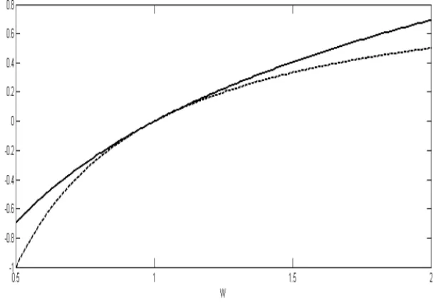
asset allocations. Given an allocation, a wealth level is associated with each outcome. The decision maker has a utility function that maps each potential wealth level to a utility. Each utility function must be increasing (more is preferred to less) and concave (incremental wealth results in decreasing incre-mental utility). We plot two utility functions in Figure 1.1. An investor (we

FIGURE 1.1: Two utility functions from the power family, with κ = 2 (more risk averse, depicted with a dashed curve) andκ= 1 (less risk averse, depicted with a solid curve).

use the terms decision maker and investor interchangeably) with the utility function indicated with the dashed curve is more risk averse than an investor with the utility function indicated with the solid curve, since, for the dashed curve, higher payoffs yield less utility and lower payoffs are more heavily pe-nalized. The two utility functions that we have depicted in this figure are both members of the well-known family of power utility functions

Uκ(W) =

W1−κ

−1

1₋κ →log(W), asκ→1, κ >0. (1.1)

In Figure 1.1, κ = 2 (more risk averse, depicted with a dashed curve) and

κ = 1 (less risk averse, depicted with a solid curve). The utility function

Uκ(W) is known to have constant relative risk aversion κ;4 the higher the

(25)

value of κ, the more risk averse is the investor with that utility function. Sometimes we will refer to a less risk averse investor as a more aggressive investor. For example, an investor with a logarithmic utility function is more aggressive than an investor with a power 2 utility function.

From a practical point of view, perhaps the most important conclusion of utility theory is that, given a probability model, a decision maker who sub-scribes to the axioms of utility theory acts to maximize his expected utility under that model. We illustrate these notions with Example 1.1, which we present in Section 1.6.5

We’d like to emphasize that, given a probability measure, and employing utility theory, there are no single, one-size-fits-all methods for

(i) allocating capital, or

(ii) measuring the performance of allocation strategies.

Rather, the decision maker allocates and assesses the performance of alloca-tion strategies based on his risk preferences. Examples 1.1 and 1.2 in Section 1.6 illustrate these points.

1.2 Model Performance Measurement

In this book we are concerned with situations where a decision maker must select or estimate a probability model. Is there a single, one-size-fits all, best model that all individuals would prefer to use, or do risk preferences enter into the picture when assessing model performance? If risk preferences do indeed enter into model performance measurement, how can we estimate models that maximize performance, given specific risk preferences? We shall address the second question (model estimation) briefly in Section 1.3 of this introduc-tion (and more thoroughly in Chapter 10), and the first (model performance measurement) in this section (and more thoroughly in Chapter 8).

We incorporate risk preferences into model performance measurement by means of utility theory, which, as we have seen in the previous section, allows for the quantification of these risk preferences. In order to derive explicit model performance measures, we will need two more ingredients:

(i) a specific setting, in which actions can be taken and a utility can be associated with the consequences, and

5_{Some of the examples in this introduction are a bit long and serve to carefully illustrate}

(26)

Introduction 5

(ii) a probability measure under which we can compute the expected utility of the decision maker’s actions.

Throughout most of this book, we choose as ingredient (i) a horse race (see Chapter 3 for a detailed discussion of this concept), in which an investor can place bets on specific outcomes that have defined payoffs. We shall also discuss a generalization of this concept to a so-called incomplete market, in which the investor can bet only on certain outcomes or combinations of outcomes. In this section we refer to both settings simply as the market setting.

As ingredient (ii) we choose the empirical measure (frequency distribution) associated with an out-of-sample test dataset. The term out-of-sample refers to a dataset that was not used to build the model. This aspect is important in practical situations, since it protects the model user to some extent from the perils of overfitting, i.e., from models that were built to fit a particular dataset very well, but generalize poorly. Example 1.3 in Section 1.6 illustrates how the problem of overfitting can arise.

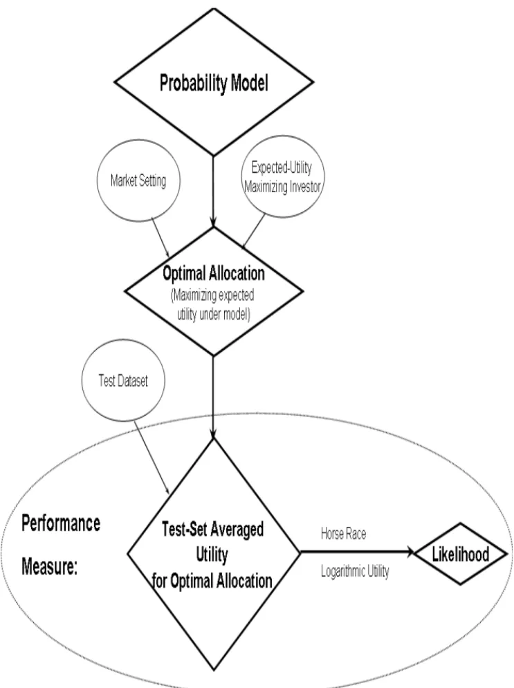
Equipped with utility theory and the above two ingredients, we can state the following model performance measurement principle, which is depicted in Figure 1.2.

Model Performance Measurement Principle:Given

(i) an investor with a utility function, and

(ii) a market setting in which the investor can allocate,

the investor will allocate according to the model (so as to maximize his expected utility under the model).

We will then measure the performance of the candidate model for this in-vestor via the average utility attained by the inin-vestor on an out-of-sample test dataset.

We note that somebody who interprets probabilities from a frequentist point of view might want to replace the test dataset with the “true” probability measure.6 The problem with this approach is that, even if one believed in the existence of such a “true” measure, it is typically not available in practice. In this book, we do not rely on the concept of a “true” measure, although we shall use it occasionally in order to discuss certain links with the frequentist interpretation of probabilities, or to interpret certain quantities under a hy-pothetical “true” measure. The ideas described here are consistent with both a frequentist or a subjective interpretation of probabilities.

The examples in Section 1.6 illustrate how the above principle works in practice. It can be seen from these examples that risk preferences do indeed matter, i.e., that decision makers with different risk preferences may prefer

6_{One can think of the “true” measure as a theoretical construct that fits the relative}

(27)

(28)

Introduction 7

different models.7_{The intuitive reason for this is that different decision makers}

possess

(i) different levels of discomfort with unsuccessful bets, and

(ii) different levels of satisfaction with successful bets.

This point has important practical implications; it implies that there is no single, one-size-fits-all, best model in many practical situations.

1.2.1 Complete versus Incomplete Markets

This section is intended for readers who have a background in financial modeling, or are interested in certain connections between financial model-ing and the approach that we take in this book. Financial theory makes a distinction between

(i) complete markets (where every conceivable payoff function can be repli-cated with traded instruments) — perhaps the simplest example is the horse race, where we can wager on the occurrence of each single state individually, and

(ii) incomplete markets.

In the real world, markets are, in general, incomplete. For example, given a particular stock, it is not, in general, possible to find a trading strategy involving one or more liquid financial instruments that pays $1 only if the stock price is exactly $100.00 in one year’s time, and zero otherwise. Even though real markets are typically incomplete, much financial theory has been based on the idealized complete market case, which is typically more tractable. As we shall see in Chapter 8, the usefulness of the distinction between the complete and incomplete market settings extends beyond financial problems — this distinction proves important with respect to measuring model per-formance. In horse race markets, the allocation problem can be solved via closed-form or nearly closed-form formulas, with an associated simplification of the model performance measure; in incomplete markets, it is necessary to rely to a greater extent on numerical methods to measure model performance.

1.2.2 Logarithmic Utility

We shall see in Chapter 8 that, for investors with utility functions in a logarithmic family, and only for such investors, in the horse race setting, the utility-based model performance measures are equivalent to the likelihood

7_{We shall show later in this book that all decision makers would agree that the “true”}

(29)

from classical statistics, establishing a link between our utility-based formu-lation and classical statistics. This link is depicted in Figure 1.2.

1.3 Model Estimation

As we have seen, different decision makers may prefer different models. This naturally leads to the notion that different decision makers may want to build different models, taking into account different performance measures. In light of this notion, we formulate the following goals:

(i) to discuss how, by starting with the model performance measurement principle of Section 1.2, we are led to robust methods for estimating models appropriate for individual decision makers, and

(ii) to establish links between some traditional information-theoretic and statistical approaches for estimating models and the approach that we take in this book, and

(iii) to briefly compare the problem settings in this book with those typi-cally used in probability model estimation and certain types of financial modeling.

To keep things as simple as possible, we (mostly) confine the discussion in this introduction to discrete, unconditional models.8 _{In the discussion that}

follows, before addressing the main goals of this section, we shall first review some traditional information-theoretic approaches to the probability estima-tion problem.

1.3.1 Review of Some Information-Theoretic Approaches

The problem of estimating a probabilistic model is often articulated in the language of information theory and solved via maximum entropy (ME), mini-mum relative entropy (MRE), or minimini-mum mutual information (MMI) meth-ods. We shall review some relevant classical information theoretic quantities, such as entropy, relative entropy, mutual information, and their properties in Chapter 2; we shall discuss modeling via the ME, MRE, and MMI principles in Chapters 9 and 10. In this introduction, we discuss a few notions informally. LetY be a discrete-valued random variable that can take values,y, in the finite set_Ywith probabilitiespy. The entropy of this random variable is given

8_{We do consider conditional models, where there are explanatory variables with known}

(30)

Introduction 9

by the quantity

H(p)≡ −X

y

pylog(py). (1.2)

It can be shown that the entropy of a random variable can be interpreted as a measure of the uncertainty of the random variable. We note that this measure of uncertainty, unlike, for example, the variance, does not depend on the values,y∈ Y; the entropy depends only on the probabilities,py.

Given another probability measure on the same states, with probabilities, {p0

1, . . . , p0n}, the Kullback-Leibler relative entropy (we often refer to this

quan-tity as, simply, relative entropy) fromptop0is given by

D(p_kp0₎

≡X

y

pylog

_p

y

p0 y

. (1.3)

It can be shown that

(i) D(p_kp0₎

≥0, and

(ii) D(p_kp0_{) = 0 only if}_p₌_p0_.

Thus, relative entropy has some, but not all,9 of the properties associated with a distance. We note that if the measurep0is uniform on the states, i.e., if there arenelements inY, and

p0y=

1

n for ally, (1.4)

then in this special case,

D(p_kp0_{) =}

−H(p)₋log(n), (1.5) so relative entropy can be viewed as a more general quantity than entropy. Moreover, minimizing relative entropy is equivalent, in this special case, where (1.4) holds, to maximizing entropy.

LetX be a discrete-valued random variable that can take values,x, in the finite set_X with probabilitiespx. The mutual information betweenX andY

is given by

I(X;Y) =X

x,y

px,ylogpx,y

pxpy

, (1.6)

where px,y denotes the joint probability that X = xand Y = y. Thus, the

mutual information is also a special case of the relative entropy for the joint random variables X and Y, where p0

x,y = pxpy. It can be shown that the

mutual information can be interpreted as the reduction in the uncertainty of

Y, given the knowledge ofX.

9_{Relative entropy is not symmetric; more importantly, it does not satisfy the triangle}

(31)

Armed with these information-theoretic quantities, we return to the goal of formulating methods to estimate probabilistic models from data; we discuss ME, MRE, and MMI modeling.

(i) ME modeling is governed by the maximum entropy principle, under which we would seek the probability measure that is most uncertain (has maximum entropy), given certain data-consistency constraints,

(ii) MRE modeling is governed by the minimum relative entropy principle, under which we would seek the probability measure satisfying certain data-consistency constraints that is closest (in the sense of relative en-tropy) to apriormeasure, p0_{; this prior measure can be thought of as}

a measure that one might be predisposed to use, based on prior belief, before coming into contact with data, and

(iii) MMI modeling is governed by the minimum mutual information prin-ciple, under which we would seek the probability measure satisfying certain data-consistency constraints, whereX provides the least infor-mation (in the sense of mutual inforinfor-mation) aboutY. If the marginal distributions,px and py, are known, then the MMI principle becomes

an instance of the MRE principle.

For ME, MRE, and MMI modeling, the idea is that the data-consistency constraints reflect the characteristics that we want to incorporate into the model, and that we want to avoid introducing additional (spurious) charac-teristics, with the specific means for avoiding introducing additional (spuri-ous) characteristics described in the previous paragraph. Since entropy and mutual information are special cases of relative entropy, the principles are indeed related, though the interpretations described above might seem a bit disparate.

1.3.1.1 Features

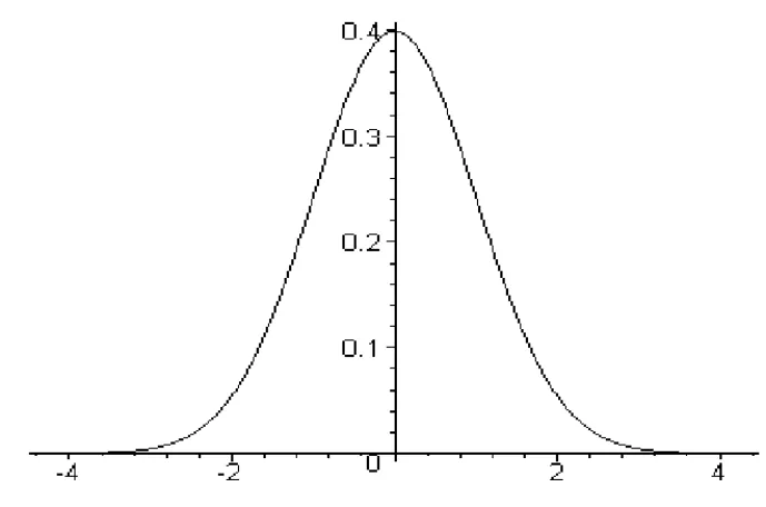
The aforementioned data-consistency constraints are typically expressed in terms of features. Formally, a feature is a function defined on the states, for example, a polynomial feature likef1(y) =y2, or a so-called Gaussian kernel

feature, with centerµand bandwidth,σ

f2(y) =e−

(y−µ)2 2σ2 .

The model,p, can be forced to be consistent with the data, for example via a series ofJ constraints

(32)

Introduction 11

where ˜p denotes the empirical measure.10 _{We can think of the expectation}

under the empirical measure on the right hand side of (1.7) as the sample average of the feature values.

Thus, by taking empirical expectations of features, we garner information about the data, and by enforcing constraints (1.7), we impose consistency of the model with the data.

1.3.1.2 The MRE Problem

The MRE problem formulation is given by

minimizeD(p_kp0_{) with respect to}_{p ,} _(1.8)

subject to data-consistency constraints, for example,

Ep[fj] =Ep˜[fj], j= 1, . . . , J. (1.9)

The solution to this problem is robust, in a sense that we make precise in Section 1.2 and Chapter 10.

1.3.1.3 The ME Problem

The ME problem formulation is given by

maximizeH(p) with respect top , (1.10)

subject to data-consistency constraints, for example,

Ep[fj] =Ep˜[fj], j= 1, . . . , J. (1.11)

As a special case of the MRE problem, the solution of the ME problem inherits the robustness of the MRE problem solution.

1.3.1.4 The MMI Problem

Under the MMI problem formulation, we seek the probability measure that minimizes the mutual information subject to certain expectation con-straints.11

1.3.1.5 Dual Problems

Fortunately, the MRE, ME, and MMI principles all lead to convex optimiza-tion problems. We shall see that each of these problems has a corresponding

dual problem which yields the same solution. In many cases (for example,

10_{Later, we shall relax the equality constraints (1.7).}

(33)

conditional probability model estimation), the dual problem is more tractable than the primal problem.

We shall see that for the MRE and ME problems,

(i) the solutions to the dual problem are members of a parametric expo-nential family, and

(ii) the dual problem objective function can be interpreted as the logarithm of the likelihood function.

These points sometimes, but not always (we shall elaborate in Chapter 10), apply to the MMI problem. Thus, the dual problem is typically interpreted as a search, over an exponential family, for the likelihood maximizing prob-ability measure.12 _{This establishes a connection between information theory}

and statistics.

1.3.2 Approach Based on the Model Performance

Measure-ment Principle of Section 1.2

In this section, we discuss how we might develop a model estimation prin-ciple around the model performance measurement prinprin-ciple of Section 1.2. At first blush, it might seem natural for an investor to choose the model that maximizes the utility-based performance measures, discussed in Section 1.2, on the data available for building the model (the training data). However, it can be shown that this course of action would lead to the selection of the em-pirical measure (the frequency distribution of the training data) — for many interesting applications,13_{a very poor model indeed, if we want our model to}

generalize well on out-of-sample data; we illustrate this idea in Example 1.3 (see Section 1.6).

Though it is, generally speaking, unwise to build a model that adheres too strictly to the individual outcomes that determine the empirical measure, the observed data contain valuable statistical information that can be used for the purpose of model estimation. We incorporate statistical information from the data into a model via data-consistency constraints, expressed in terms of features, as described in Section 1.3.1.1.

12_{Depending on the exact choice of the data-consistency constraints, the objective function}

of this search may contain an additional regularization term. We shall elaborate on this in Chapters 9 and 10.

13_{For some simple applications, for example a biased coin toss with many observations,}

(34)

Introduction 13

1.3.2.1 Robust Outperformance Principle

Armed with the notions of features and data-consistency constraints, we return to our model estimation problem. The empirical measure typically does not generalize well because it is all too precisely attuned to the observed data. We seek a model that is consistent with the observed data, in the sense of conforming to the data-consistency constraints, yet is not too precisely attuned to the data. The question is, which data-consistent measure should we select? We want to select a model that will perform well (in the sense of the model performance measurement principle of Section 1.2), no matter which data-consistent measure might govern a potential out-of-sample test set. To address this question, we consider the following game against nature14 _(which

we assume is adversarial) that occurs in a market setting.

A game against “nature”LetQdenote the set of all probability measures,

K denote the set of data-consistent probability measures, and U∗

q denote the

(random) utility that is realized when allocating (so as to maximize expected utility) under the measureq in this market setting.15

(i) (Our move) We choose a model,q∈Q; then,

(ii) (Nature’s move) given our choice of a model, and, as a consequence, the allocations we would make, “nature” cruelly inflicts on us the worst (in the sense of the model performance measurement principle of Sec-tion 1.2) possible data-consistent measure; that is, “nature” chooses the measure

p∗= arg min

p∈KEp[U

∗

q]. (1.12)

If we want to perform as well as possible in this game we will seek the solution of

q∗= arg max

q∈Q minp∈KEp[U

∗

q]. (1.13)

By solving (1.13), we estimate a measure that (as we shall see later) conforms to the data-consistency constraints, and is robust, in the sense that the ex-pected utility that we can derive from it will be attained, or surpassed, no mat-ter which data-consistent measure “nature” chooses. The resulting estimate therefore, in particular, avoids being too precisely attuned to the individual observations in the training dataset, thereby mitigating overfitting.16

14_{This game is a special case of a game in Gr¨}_{unwald and Dawid (2004), which was preceded}

by the “log loss game” of Good (1952).

15_{We note that we are speaking informally here, since we have not specified the market}

setting or how to calculateU∗

q. We shall discuss these issues more precisely in the remainder

of the book.

16_{This strategy does not guarantee a cure to overfitting, though! If there are too many}

(35)

This game can be further enriched by introducing a rival, who allocates according to the measure q0

∈Q.17 _{In this case, we would seek the solution}

according to the robust outperformance principle:

Robust Outperformance Principle

We seek

q∗= arg max

q∈Qminp∈KEp[U

∗

q −Uq∗0]. (1.14)

Estimatingq∗_{would allow us to to maximize the worst-case outperformance}

over our competitor (who allocates according to the measureq0

∈Q), in the presence of a “nature” that conforms to the data-consistency constraints and tries to minimize our outperformance (in the sense of the model performance measurement principle of Section 1.2) over our rival.

Jaynes (2003), page 431, has pointed out that “this criterion concentrates attention on the worst possible case regardless of the probability of occurrence of this case, and it is thus in a sense too conservative.” In our view, this may be so, given a fixed collection of features. However, by enriching the collection of features, it is always possible to go too far in the other direction, overly constraining the set of measures consistent with the data, and estimating a model that is too aggressive. We shall have more to say about ways to attempt to tune (optimally) the extent to which the data are consistent with the model in Section 1.3.5 and Chapter 10.

We note that this formulation has been cast entirely in the language of utility theory. The model that is produced is therefore specifically tailored to the risk preferences of the model user with utility function U. We also note that we have not made use of the concept of a “true” measure in this formulation.

1.3.2.2 Minimum Market Exploitability Principle

As we shall see in Chapter 10, under certain technical conditions, it is pos-sible to reverse the order of the max and min in the robust outperformance principle. Moreover, as we shall see in Chapter 10, subject to regularity con-ditions, by solving the resulting minimax problem, we obtain the solution to the maxmin problem (1.14) arising from the robust outperformance principle. By reversing the order of the max and min in (1.14), we obtain the minimum market exploitability principle:

Minimum Market Exploitability Principle

can arise. We shall discuss these issues, and countermeasures that can be taken to fur-ther protect against overfitting, at greater length below in this introduction, as well as in Chapters 9 and 10.

(36)

Introduction 15

We seek

p∗_{= arg min}

p∈Kmaxq∈QEp[U

∗

q −Uq∗0]. (1.15)

Here,

Ep[Uq∗−Uq∗0] (1.16)

can be interpreted as the gain in expected utility, for an investor who allocates according to the modelq, rather thanq0_{, when the “true” measure is}_p_{. Under}

the minimum market exploitability principle, we seek the data-consistent mea-sure,p, that minimizes the maximum gain in expected utility over an investor who uses the modelq0_{. After a little reflection, this principle is consistent with}

a desire to avoid overfitting. The intuition here is that the data-consistency constraints completely reflect the characteristics of the model that we want to incorporate, and that we want to avoid introducing additional (spurious) characteristics. Any additional characteristics (beyond the data-consistency constraints) could be exploited by an investor; so, to avoid introducing addi-tional such characteristics, we minimize the exploitability of the market by an investor, given the data-consistency constraints.

Fortunately, as we shall see in Chapter 10, the minimum market exploitabil-ity principle leads to a convex optimization problem with an associated dual problem that can be solved robustly via efficient numerical techniques. More-over, as we shall also see in Chapter 10, this dual problem can be interpreted as a utility maximization problem over a parametric family, and can be solved robustly via efficient numerical techniques.

By virtue of their equivalence, both the minimum market exploitability principle and the robust outperformance principle lead us down the same path; both lead to a tractable approach to estimate statistical models tailor-made to the risk preferences of the end user.

1.3.3 Information-Theoretic Approaches Revisited

As we shall see in Chapter 7, the quantity maxq∈QEp[Uq∗−Uq∗0] in (1.15) is

a generalization of relative entropy, with a clear economic interpretation. In particular, we shall see in Chapter 7, that the relative entropy,D(pkp0_{), can}

be interpreted as the gain in expected utility, for a logarithmic utility investor who allocates in a horse race on the states according to the “true” measure

p, rather than the measurep0_.

We shall also see in Chapter 10 that the minimum market exploitability principle, in fact, includes as special cases the maximum entropy (ME) princi-ple, the minimum relative entropy (MRE) principrinci-ple, and the minimum mutual information (MMI) principle, and that all of these principles can be expressed in economic terms.

(37)

that we want to avoid introducing could be exploited by an investor; so, to avoid introducing additional characteristics beyond the data-consistency constraints, we minimize the exploitability of the market by an investor, given the data-consistency constraints. In particular, as we shall see in Chapter 10,

(i) the ME principle can be viewed as the requirement that, given the data-consistency constraints, our model have as little (spurious) expected logarithmic utility as possible,

(ii) the MRE principle can be viewed as the requirement that, given the data-consistency constraints, our model have as little (spurious) ex-pected logarithmic utility gain as possible over an investor who allocates to maximize his expected utility under the prior measure, and

(iii) the MMI principle can be viewed as the requirement that, given the data-consistency constraints, our model have as little (spurious) expected logarithmic utility gain as possible over an investor who allocates to maximize his expected utility without making use of the information given by the realizations ofX.

We believe that this economic intuition provides a convincing and unifying rationale for the ME, MRE, and MMI principles.

We shall also see that

(i) for the ME, MRE, and certain MMI problems,18 _{the objective function}

of the dual problem can be interpreted as the expected utility of an investor with a logarithmic utility function, so the dual problem can be formulated as the search, over an exponential family of measures, for the measure that maximizes expected (logarithmic) utility, or, equivalently, maximizes the likelihood, and that

(ii) for the ME, MRE, and MMI problems, by construction, the solutions possess the optimality and robustness properties discussed in Section 1.3.2.1 — they provide maximum expected utility with respect to the worst-case measures that conform to the data-consistency constraints.

For more general utility functions, we would obtain more general versions of the ME, MRE, and MMI principles; in this book, when we discuss more general utility functions, we shall concentrate on more general version of the MRE principle, rather than the ME or MMI principles.

1.3.4 Complete versus Incomplete Markets

As indicated in Section 1.2.1, there is an important distinction between the complete horse race setting and the more general incomplete market setting. In

(38)

Introduction 17

the more tractable horse race setting, with data-consistency constraints under which the feature expectations under the model are related to the feature expectations under the empirical measure, the generalized relative entropy principle has an associated dual problem that can be viewed as an expected utility maximization over a parametric family. We are not aware of similar results in incomplete market settings.

1.3.5 A Data-Consistency Tuning Principle

As we have discussed, the above problem formulations bake in a robust out-performance over an investor who allocates according to the prior, or bench-mark model,givena set of data-consistency constraints. But how, given a set of feature functions,19_{can we formulate data-consistency constraints that will}

prove effective?

The simplest (and most analytically tractable) way to generate data-consistency constraints from features is to require that the expectation of the features under the model be exactly the same as the expectation under the empirical measure (the frequency distribution of the training data). How-ever, this requirement does not always lead to effective models. Two of the things that can go wrong with this approach, depending on the number and type of features and the nature of the training data, are

(i) the feature expectation constraints are not sufficiently restrictive, re-sulting in a model that has not “learned enough” from the data, and

(ii) the feature expectation constraints are too restrictive, resulting in a model that has learned “too much” (including noise) from the data.

In case (i), where the features are not sufficiently restrictive, we can add new features. In case (ii), where the features are too restrictive, we can relax them. By controlling the degree of relaxation in the feature expectation constraints, we can control the tradeoff between consistency with the data and the extent to which we can exploit the market, relative to the performance of our rival investor. In the end, in this case, our investor chooses the model that best balances this tradeoff, with respect to the model performance measurement principle of Section 1.2 applied to an out-of-sample dataset, as indicated in the following principle

Data-Consistency Tuning Principle

Given a family of data constraint sets indexed by the parameter α, let q∗(α)

denote the model selected under one of the equivalent principles of Section 1.3.2 as a function of α. We tune the level of data-consistency to maximize

19_{In this book, we do not discuss methods to generate features — we assume that they are}

(39)

(overα) the out-of-sample performance under the performance measurement principle of Section 1.2.

1.3.6 A Summary Diagram for This Model Estimation,

Given a Set of Data-Consistency Constraints

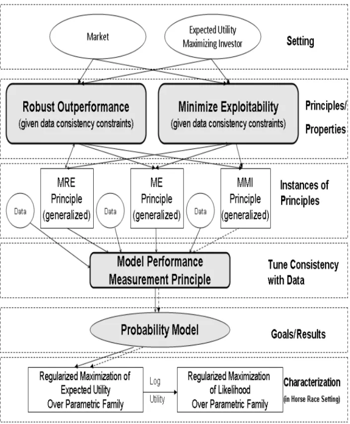
We display some of the relationships discussed above in Figure 1.3, where

(i) we have used a dashed arrow to signify that the MMI principle some-times, but not always (we shall elaborate in Chapter 10), leads to a utility maximization problem over a parametric family, and

(ii) we have used bi-directional arrows between the generalized MRE princi-ple and the robust outperformance and minimum market exploitability principles, since, as we shall see in Chapter 10, all three principles are equivalent.

1.3.7 Problem Settings in Finance, Traditional Statistical

Modeling, and This Book

In this section, which may be of particular interest to readers with a back-ground in financial modeling, we compare the problem settings used in this book with problem settings used in finance and traditional statistical model-ing.

Though we use methods drawn from utility theory, the problems to which we apply these methods are (statistical) probability model estimation prob-lems, rather than more typical financial applications of utility theory. One such application — the least favorable market completion principle (discussed in Section 11.2), which is used in finance to price contingent claims20 _{— is}

quite similar in spirit to our minimum market exploitability principle. As we shall see, (statistical) probability model estimation problems and the pricing problems from finance can be structurally similar.

In the case of contingent claim pricing problems, given the statistical sure on the system (in finance, this measure is often called the physical sure, or the real-world measure) the modeler seeks a different probability mea-sure, a probability measure consistent with known market prices (a so-called pricing measure, or risk-neutral measure).

In the case of traditional probability model estimation problems, outside of finance, the modeler seeks a statistical (real-world) measure consistent with certain data-consistency constraints. Thus, the traditional statistical modeler

20_{Contingent claims are financial instruments with contractually specified payments that}

(40)

Introduction 19

(41)

seeks a statistical (real-world) measure, and is, typically, not at all concerned with pricing measures; the contingent claim modeler assumes that the statis-tical (real-world) measure is known, and seeks a pricing measure.

In particular, in the horse race setting, with payoffs specified for each state,

(i) the contingent claim modeler essentially already has the pricing measure (which can easily be determined from the payoffs) and is able to price any contingent claim by reconstructing its payoff in terms of the horse race payoffs,

(ii) the traditional statistical modeler is, typically, not influenced by the payoffs, and must take whatever steps are necessary to find the statistical measure, and

(iii) we use the payoffs, together with utility theory, as described in the preceding sections, to evaluate model performance and estimate mod-els (given data-consistency constraints) for expected utility maximizing investors.

1.4 The Viewpoint of This Book

As discussed in the preceding sections, we take the viewpoint of a decision maker who uses a probability model to make decisions in an uncertain en-vironment. We believe that this viewpoint is natural, appropriate for many practical problems, and leads to intuitive, desirable, and tractable model per-formance measurement and model construction principles. When taking this point of view, it is relatively straightforward to construct, generalize, and shed light on some well-known principles from information theory, finance, and sta-tistical learning. Moreover, the mindset and language adopted in this book lead to various nontraditional methods that can be brought to bear on prac-tical problems. These nontraditional methods, some of which are discussed in this book, can be used to

(i) relate the performance of probability models to the risk preferences of the model user,

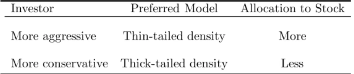
(ii) build robust probability models that are custom-tailored to the model user’s risk preferences (which can, depending on the investor’s risk pref-erences, result in relatively elegant representations of fat-tailed, yet flex-ible distributions),

(42)

Introduction 21

(iv) quantify the impact of information exploitability on the performance of a probability model (measuring model performance in incomplete financial markets), and

(v) derive robust performance measures for regression models.

1.5 Organization of This Book

Chapters 8 and 10 constitute the crux of this book; each of these chapters depends on the chapters that precede it.

In Chapter 2, we review mathematical preliminaries from probability theory, convex optimization (all of the methods for building probabilistic models that we discuss in this book require solution to convex programming problems), and information theory. These are the building blocks that we use in later chapters.

In Chapter 3, we review the horse race setting, which is also known as a complete market. This is a particularly tractable and simple “market” setting — used heavily throughout this book — in which we can consider model performance and model building from a decision-theoretic point of view.

In Chapter 4, we review elements of utility theory. Utility theory provides a framework that we use to describe investor risk preferences. Expected utility maximization (von Neumann and Morgenstern (1944)) allows for plausible and practical model performance measurement and provides a goal for model construction.

In Chapter 5, we discuss an expected utility maximizing investor who bets in a horse race type market. In particular, we introduce the notion of compat-ibility between the utility function, the horse race market, and the probability measure. When the utility function, the market, and the probability measure are compatible, there is always an optimal allocation.

In Chapter 6, we discuss select popular methods for measuring model perfor-mance. In particular, we discuss the likelihood principle, the likelihood ratio, and the Neyman-Pearson Lemma, and draw connections between likelihood and the horse race.

In Chapter 7, we discuss information theory from a decision-theoretic point of view. This chapter starts by observing that there are decision-theoretic interpretations (in terms of an investor with a particular utility function) for fundamental information theoretic quantities. We then note that by gen-eralizing the utility function, we obtain more general information theoretic quantities, which we explore.

(43)

In Chapter 9, we review select methods for learning probabilistic models from data, including maximum likelihood inference and regularized maximum likelihood inference, including the ridge and lasso models. We also discuss Bayesian inference and minimum relative entropy methods.

In Chapter 10, we develop the model learning problem in the horse race context. Based on the general principals introduced in the introduction to this book, we formulate explicit primal and dual problems.

In Chapter 11, we discuss various extensions of the material in earlier chap-ters. We discuss model performance measures for leveraged investors, model performance and estimation in incomplete markets, and model performance measurement for regression models.

In Chapter 12, we discuss applications to four important financial modeling problems, a breast cancer model, and a text categorization problem.

1.6 Examples

Example 1.1 Four gamblers allocate to a coin toss

In this example, we see that given a probability measure, and employing utility theory, there are no single, one-size-fits-all methods for allocating cap-ital.

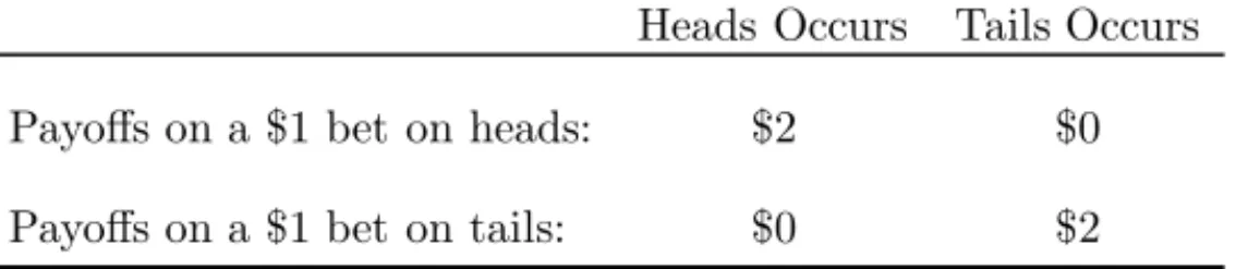
The specific setting, which is summarized in Table 1.1, is as follows.

TABLE 1.1:

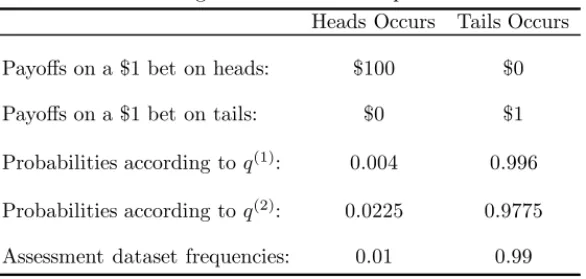
Four gamblers (completely risk averse, expectation maximizing or linear utility, log utility, and power 2 utility) allocate to a coin toss. The probability of heads is.51.

Heads Occurs Tails Occurs

Payoffs on a $1 bet on heads: $2 $0

Payoffs on a $1 bet on tails: $0 $2

The payoff for a $1 bet on heads is $2 if heads occurs and zero otherwise; the payoff for a $1 bet on tails is $2 if tails occurs and zero otherwise. Each gambler must allocate his wealth to heads and/or tails. The probability of heads is known to be .51. How should a gambler allocate his capital? That depends on the gambler’s risk preferences.

(44)

Introduction 23

case, his total payoff will always be exactly $1, no matter whether the coin toss results in heads or tails.

Suppose that, at the other extreme, our second gambler will do whatever it takes to maximize the expected payoff after a single play of the game. If he allocates the fraction,b, of his wealth to heads and the fraction 1₋b to tails, he would allocate his wealth so as to solve the problem

max

{b:0≤b≤1}[0.51∗2b+ 0.49∗2(1−b)]. (1.17)

This expected payoff maximizing gambler will choose b = 1, i.e., he will al-locate his entire wealth to heads, with expected payoff 0.51_∗2 = 1.02. We note that though this strategy maximizes the expected wealth gain on a single play, in the long run, under repeated play, the strategy of allocating all of the wealth to heads is almost surely a recipe for ruin. Eventually, almost surely, a tail will occur and the gambler will lose all of his wealth. This gambler is oblivious to that risk.

If a gambler subscribes to the axioms of utility theory, he would allocate so as to maximize his expected utility. Such a gambler, allocating fraction b of his wealth to heads and the fraction 1−bto tails, would solve the problem

max

{b:0≤b≤1}[0.51∗U(2b) + 0.49U(2(1−b))]. (1.18)

We note that a gambler with the linear utility function, U(W) =W, would formulate precisely the optimization problem (1.17). Thus the expectation maximizing gambler can be characterized by the utility functionU(W) =W. Suppose that our third gambler has the utility function U(W) =log(W). He would solve the problem

max

b [0.51 log(2b) + 0.49 log(2(1−b))]. (1.19)

It is easy to verify, by calculus, that the investor with the utility U(W) =

log(W) will allocate the fractionb∗_{= 0}_._{51 to heads and 0}_._{49 to tails.}

Suppose that our fourth gambler’s utility function is given by the power utility withκ= 2. He would solve the problem

max

b

0.51(2b)

1−2

−1 1₋2 + 0.49

(2(1₋b))1−2

−1 1₋2

. (1.20)

After setting the derivative to zero, solving, and checking the second deriva-tive, we see that this investor will allocate b∗ _{= 0}_._{505 to heads and 0}_.₄₉₅

(45)

wealth growth rate for the completely risk averse decision maker is zero, since his wealth never changes, with no possibility of drawdowns.

Example 1.2 Two of our gamblers rank wealth distributions

In this example, we shall see that different investors may rank wealth dis-tributions differently, depending on their risk preferences.

In the same setting as Example 1.1 (see Table 1.1), after repeated play, with heads occuring 51% of the time, we suppose that each of our decision makers, with log utility and power, withκ= 2, utility functions, respectively, can choose among the wealth distributions generated by the two strategies

b∗ _{= 0}_._{51, and} _b∗ _{= 0}_._{505. We assume that these decision makers measure}

the success of the strategies in a manner consistent with the axioms of util-ity theory — by computing expected utilutil-ity with respect to the probabilities actually experienced. This formulation leads to the quantities that we max-imized in (1.19) and (1.20). As we have already seen from the optimization problems, the log utility investor will prefer the wealth distribution generated by the allocationsb∗_{= 0}_._{51 and the power 2 decision maker prefers the wealth}

distribution generated byb∗_{= 0}_._505.

Example 1.3 An overfit model

In this example, we shall see that the empirical measure can be a very poor model.

Let the random variableX denote the daily return of a stock. We observe the daily stock returnsx1, . . . , x10, over a two week period (10 trading days).

The empirical measure is then

prob(X=x) =

1

10, ifx∈ {x1, . . . , x10}, and

0, otherwise, (1.21)

assuming that each of the returns is unique. This model reflects the train-ing data perfectly, but will fail out-of-sample, since it only attaches nonzero probability to events that have already occurred. If this model is to be be-lieved, then it would make sense to risk all on the bet thatxn∈ {x1, . . . , x10},

for n >10, a strategy doomed to fail when a previously unobserved return (inevitably) occurs.

CRC Press Utility Based Learning from Data 2010 RETAiL EBook pdf

Utility-Based

Learning from Data

Chapman & Hall/CRC

Machine Learning & Pattern Recognition Series

SERIES EDITORS

Ralf Herbrich and Thore Graepel

Microsoft Research Ltd.

Cambridge, UK

AIMS AND SCOPE

This series reflects the latest advances and applications in machine learning

and pattern recognition through the publication of a broad range of reference

works, textbooks, and handbooks. The inclusion of concrete examples,

appli-cations, and methods is highly encouraged. The scope of the series includes,

but is not limited to, titles in the areas of machine learning, pattern

recogni-tion, computational intelligence, robotics, computational/statistical learning

theory, natural language processing, computer vision, game AI, game theory,

neural networks, computational neuroscience, and other relevant topics, such

as machine learning applied to bioinformatics or cognitive science, which

might be proposed by potential contributors.

PUBLISHED TITLES

MACHINE LEARNING: An Algorithmic Perspective

Stephen Marsland

HANDBOOK OF NATURAL LANGUAGE PROCESSING,

Second Edition

Nitin Indurkhya and Fred J. Damerau

UTILITY-BASED LEARNING FROM DATA

Craig Friedman and Sven Sandow

Chapman & Hall/CRC

Machine Learning & Pattern Recognition Series

Utility-Based

Learning from Data

Craig Friedman

Sven Sandow

Chapman & Hall/CRC

Machine Learning & Pattern Recognition Series

SERIES EDITORS

Ralf Herbrich and Thore Graepel

Microsoft Research Ltd.

Cambridge, UK

AIMS AND SCOPE

This series reflects the latest advances and applications in machine learning

and pattern recognition through the publication of a broad range of reference

works, textbooks, and handbooks. The inclusion of concrete examples,

appli-cations, and methods is highly encouraged. The scope of the series includes,

but is not limited to, titles in the areas of machine learning, pattern

recogni-tion, computational intelligence, robotics, computational/statistical learning

theory, natural language processing, computer vision, game AI, game theory,

neural networks, computational neuroscience, and other relevant topics, such

as machine learning applied to bioinformatics or cognitive science, which

might be proposed by potential contributors.

PUBLISHED TITLES

MACHINE LEARNING: An Algorithmic Perspective

Stephen Marsland

HANDBOOK OF NATURAL LANGUAGE PROCESSING,

Second Edition

Nitin Indurkhya and Fred J. Damerau

UTILITY-BASED LEARNING FROM DATA

Craig Friedman and Sven Sandow

Chapman & Hall/CRC

Machine Learning & Pattern Recognition Series

Utility-Based

Learning from Data

Craig Friedman

Sven Sandow

Contents

Preface

Acknowledgments

Disclaimer

Chapter 1

Introduction

1.1

Notions from Utility Theory

1.2

Model Performance Measurement

1.2.1

Complete versus Incomplete Markets

1.2.2

Logarithmic Utility

1.3