5127.pdf

(1)

Analysis and Visualization of Local Phylogenetic Structure

within Species

Jeremy R. Wang

A dissertation submitted to the faculty of the University of North Carolina at Chapel Hill in partial fulfillment of the requirements for the degree of Doctor of Philosophy in the Depart-ment of Computer Science.

Chapel Hill 2013

Approved by:

Leonard McMillan

Wei Wang

Fernando Pardo-Manuel de Villena

Gary Churchill

Vladimir Jojic

(2)

c

(3)

Abstract

JEREMY R. WANG. Analysis and Visualization of Local Phylogenetic Structure within Species.

(Under the direction of Leonard McMillan.)

While it is interesting to examine the evolutionary history and phylogenetic relationship

between species, for example, in a sort of “tree of life”, there is also a great deal to be learned

from examining population structure and relationships within species. A careful

descrip-tion of phylogenetic reladescrip-tionships within species provides insights into causes of phenotypic

variation, including disease susceptibility. The better we are able to understand the patterns

of genotypic variation within species, the better these populations may be used as models to

identify causative variants and possible therapies, for example through targeted genome-wide

association studies (GWAS). My thesis describes a model of local phylogenetic structure,

how it can be effectively derived under various circumstances, and useful applications and

visualizations of this model to aid genetic studies.

I introduce a method for discovering phylogenetic structure among individuals of a

pop-ulation by partitioning the genome into a minimal set of intervals within which there is no

evidence of recombination. I describe two extensions of this basic method. The first allows it

to be applied to heterozygous, in addition to homozygous, genotypes and the second makes

it more robust to errors in the source genotypes.

I demonstrate the predictive power of my local phylogeny model using a novel method

for genome-wide genotype imputation. This imputation method achieves very high accuracy

- on the order of the accuracy rate in the sequencing technology - by imputing genotypes in

(4)

Comparative genomic analysis within species can be greatly aided by appropriate

visual-ization and analysis tools. I developed a framework for web-based visualvisual-ization and analysis

of multiple individuals within a species, with my model of local phylogeny providing the

underlying structure. I will describe the utility of these tools and the applications for which

(5)

Acknowledgments

I would like to thank my advisor, Leonard McMillan, for his constant support and advice, my

parents for encouraging me in my love and pursuit of computers and education, my brilliant

wife for her love and support, and my twin brother for talking about any and every geeky

thing I came up with, and for reading and helping me revise this document. He hates that

(6)

List of Figures

1.1 Tree of life . . . 2

1.2 Murinae phylogenetic tree . . . 3

1.3 Neighbor-joining tree of laboratory mice . . . 4

1.4 Genomic chromosome structure . . . 7

1.5 Reduction of DNA sequences to binary SNPs . . . 8

2.1 CU ber covers . . . 22

2.2 CU ber cores and flagging SNPs . . . 24

2.3 Construction of perfect phylogeny and neighbor-joining trees. . . 27

2.4 Relationship betweenCLR,CRL, andCM ax . . . 29

2.5 Illustration of proofs . . . 34

2.6 Construction ofCM ax . . . 35

2.7 Distribution of cover sizes over genotypes . . . 40

2.8 Interval cover run times . . . 43

2.9 Interval sizes for the CEU population . . . 45

2.10 Max-k run times and statistics . . . 46

3.1 Imputation strain sets . . . 54

3.2 Imputation workflow . . . 56

3.3 Phylogenetic tree construction . . . 57

3.4 Examples of imputation confidence . . . 58

3.5 Leaf/haplotype sharing matrix . . . 64

4.1 Visualization overview . . . 77

(11)

4.3 Subspecific origin and haplotype diversity . . . 80

4.4 Highlight and zoom functionality . . . 80

4.5 Closeup feature selection . . . 81

4.6 Closeup of SNPs and genotypes . . . 83

4.7 Haplotype block mosaic . . . 84

4.8 Haplotype sorting . . . 85

4.9 Subspecific origin with diagnostic SNPs . . . 88

4.10 Heterozygosity track . . . 89

4.11 Compatible interval tracks . . . 90

4.12 Identity by descent track . . . 90

4.13 Intervals, haplotypes, and a tree . . . 92

5.1 Interval detection growth . . . 97

5.2 Simulated interval detection growth . . . 98

5.3 Interval detection by error rate . . . 98

5.4 Multiple least-squares fit of Sanger intervals . . . 99

5.5 SimulatedR5 CM ax−k relaxation . . . 104

5.6 Interval Set Overlap . . . 107

5.7 Rrconcordance results . . . 108

5.8 Accuracy ofRrCM ax in simulation . . . 109

5.9 Real Example ofR5CM ax−krelaxation . . . 110

5.10 Transitions and Transversions . . . 113

5.11 Interval growth rate for transitions and transversions . . . 114

(12)

List of Tables

1.1 Definition of terms . . . 6

3.1 Imputation confidence in 88 strains . . . 69

3.2 Error in leave-one-out imputation . . . 69

3.3 Imputation accuracy of LG/J and SM/J . . . 69

3.4 Imputation method comparison . . . 70

3.5 Strains contributing unrepresented haplotypes . . . 70

3.6 Strains with the highest variation . . . 70

5.1 Imputation results usingRrCM ax−k . . . 111

(13)

Chapter 1 Introduction

Phylogenies describe the genetic relationships between species or individuals. Inferring these

relationships helps us better understand genetic similarities and differences which may drive

phenotypic variation and describe the organism’s history. Inter-species phylogenies -

evo-lutionary trees - describe the derivation of genomes between species. Intra-species

phy-logenetic structure describes the more complex multiple-inheritance relationships between

individuals in an interbreeding population.

Genomic structure can be represented, at a high level, as a mosaic of ancestral genomes.

This representation simplifies genome-wide analyses and is more robust than typical analyses

based on point markers. Relationships between individuals can be used to assess

genome-wide associations. I will first discuss phylogenetics and how my approach is related to

higher-level genomic structure. I will then define the genomic features and events forming the basis

for my model of local phylogenetic structure.

1.1 Phylogenetics

The study of phylogenetics aims to describe the relationships between phyla, species, or

individuals by their shared genetic material. Phylogenetics has been a major area of study

(14)

evolutionary tree of life, with branches implying division between entire groups of organisms.

In a phylogeny among species, these branches indicate “speciation” events where a species

diverged to evolve into two or more different species. Species do not interbreed, so there is

no recombination between their genomes. Figure 1.1 shows an evolutionary tree describing

the phylogenetic structure of a large portion of life on earth.

Figure 1.1: A phylogenetic tree indicating the evolutionary descent of organisms, including the top two taxonomic levels: Domain, including Eukaryotes (red), Bacteria (green), and Archaea (blue), and Kingdom, the most familiar of which will be Animals, Plants, and Fungi. This type of phylogenetic tree is rooted in the center with time progressing outward. Branches indicate the point at which groups diverged, those closer to the outside of the circle indicating more recent developments (on an evolutionary time scale). Viridae not shown. Credit Wikimedia Commons (http://commons.wikimedia.org).

Although there is considerable disagreement among biologists about the appropriate

tax-onomic levels and classifications, the schema for representing phylogenetic structure as an

evolutionary tree down to the level of species or subspecies is widely agreed-upon [93].

The input data used initially were macroscopic or microscopic characteristics (e.g.,

(15)

DNA-based phylogenies became feasible beginning with one or a few genetic markers, and

currently based on hundreds of thousands of genetic markers or full genome sequence.

Al-though the methods I will describe are general, the applications and experimental results have

focused on the laboratory mouse. Figure 1.2 shows a phylogenetic tree of a subset of the

sub-family Murinae (sub-family Muridae) including the speciesMus musculus(the house mouse) and

five known subspecies. It is at this point that we start to see a breakdown of the standard form

of evolutionary trees. Mus musculus molossinusis generally considered a hybrid of M. m.

castaneusandM. m. musculus, and thus not the result of a simple speciation event. As we

begin to consider the phylogenetic structure within species, subspecies, and populations, this

global depiction of phylogeny breaks down.

Figure 1.2: Phylogenetic tree of a subset of the subfamily Murinae (family Muridae) including the species

(16)

Phylogenetic analyses among closely related species or individuals are often determined

by some measure of global genetic similarity. For example, we can line up the genetic

se-quence of two individuals and compare them base-by-base, computing percent identity.

Us-ing a sample (individual) from each of several strains (for our purposes right now, consider

these isolated subpopulations) of common laboratory mice, we can do this kind of

compari-son then construct a phylogenetic tree by recursively merging the “nearest neighbor” - the two

strains with the highest percent identity (this is called neighbor-joining). Figure 1.3 depicts

this type of tree. While this kind and construction of tree is not strictly an evolutionary tree, it

somehow represents a phylogenetic relationship [66]. This is especially true of the placement

of SPRET, CAST, and PWK. These strains are known to predominantly representMus

spre-tus(a different but closely related species), Mus musculus castaneus, andM. m. musculus,

respectively, while the remainder of the strains are predominantly M. m. domesticus. The

tree in Figure 1.3 accurately reflects these species and subspecific divisions.

(17)

In the case of species, this general approach to phylogenetics is appropriate and effective,

mainly based on the constraint that individuals of different species cannot typically interbreed

to produce fertile offspring. The first violation can be seen at the subspecies level. Mus

musculus molossinus introduces an atypical feature into our tree because it is thought to

be a hybrid ofM. m. musculusandM. m. castaneus. In order to consider the phylogenetic

relationships within a species, subspecies, or population, one must allow for the possibility of

interbreeding. Within an interbreeding population, an individual inherits from both parents.

When we attempt to model this, we cannot construct a simple bifurcating tree as we have

done so far. What we end up with is a web of inheritance relationships. I will discuss the

factors affecting genomic inheritance within species and how I derive the local phylogeny

structure under these conditions.

1.1.1 Thesis Statement

I introduce methods for efficiently and accurately identifying compatible genomic intervals

describing local phylogenetic structure within species. These intervals represent unique local

phylogenetic trees. I show how these intervals can be used to perform accurate

genome-wide imputation and to inform genome-genome-wide association studies. I describe the design and

utility of visualization tools using local phylogenetic structure to allow effective and novel

comparative analyses between individuals. Lastly, I introduce an extension of my model of

(18)

Allele One of two or more alternative forms of a gene that arise by mu-tation and are found at the same place on a chromosome

Base-pair (bp) A pair of complementary bases in a double-stranded nucleic acid molecule

Chromosome The distinct molecular units containing all or most of the genetic material of cellular organisms

Diploid Having two sets of homologous chromosomes

Genome The genetic material of an organism

Genotype The genetic constitution of an individual organism

Haploid Having one set of distinct chromosomes, often one of each pair of homologous chromosomes

Haplotype A group of alleles of different genes on a single chromosome Heterozygous Having dissimilar alleles at corresponding chromosomal loci Homozygous Having identical alleles at corresponding chromosomal loci Phylogenetics The study of evolutionary relatedness among groups of

organ-isms

Recombination The rearrangement of genetic material, esp. by crossing over in chromosomes

Single-Nucleotide Polymorphism (SNP)

Genetic variation in DNA where a single nucleotide is altered

Table 1.1: Definition of terms

1.2 Genetic Structure and Inheritance

1.2.1 Genomic Nomenclature

I will introduce a general notion of genetic structure, inheritance, and phenomena which

affect them as it pertains to intraspecific phylogenetic structure. The mouse genome is

ap-proximately 2.5 billion base-pairs long. Each base on the primary strand consists of a single

nucleotide, of which there are four possible choices, adenine (A), cytosine (C), guanine (G),

or thymine (T). Within a species, only a very small fraction of base-pairs vary between

in-dividuals. We call these single-nucleotide polymorphisms, or SNPs. These and other

com-monly used genomic terms are defined in Table 1.1.

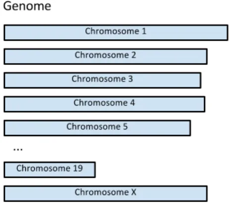
Genetic information is broken into separate functional units called chromosomes. Every

(19)

Figure 1.4:The genome is broken into blocks called chromosomes, each of which has two copies.

inherited from each parent. In mice, there are 20 pairs of chromosomes; 19 of them,

num-bered 1-19, are called autosomes and the last pair are the sex chromosomes, labeled X and Y

(see Figure 1.4). As with humans, females have an XX pair and males have an XY pair. The

collection of chromosomes makes up the genome of an individual. In naturally occurring

sexually-reproducing populations, the two copies of each chromosome are different. One is

transmitted from the mother and the other from the father.

1.2.2 Genetic Variation

One of the primary sources of genetic variation in sexually-reproducing species is mutation

(see Table 1.1). Because mutation is very rare [53], I will make a common simplifying

assumption known as the infinite-sites model [48]. This model states that mutation is

suffi-ciently rare and the genome suffisuffi-ciently long that no single position is likely to ever mutate

more than once. I will evaluate the impact of this assumption and propose a relaxation in

Chapter 5. Under this assumption, no SNP may include more than two alleles. As a result,

I will frequently simplify the representation of a haplotype to include binary alleles, ‘0’ and

‘1’, ‘0’ indicating the majority allele and ‘1’ representing the minority allele or nucleic acid

(see Figure 1.5). The infinite-sites model does not preclude the existence of heterozygosity,

(20)

‘1’. Violations of the infinite-sites model, where there have been multiple mutations at a

single base position, are called homoplasy events. In Chapter 2, I will take further advantage

of the infinite-sites model to make inferences about phylogenetic structure. We also often

ignore everything but SNPs - that is, ignore all non-variable base-pairs - when comparing

individuals.

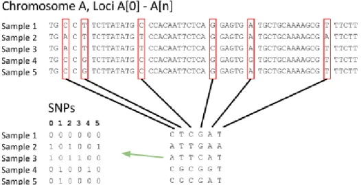
Figure 1.5:Reduction of genome sequences to binary single-nucleotide polymorphisms (SNPs). Most loci in the genome do not vary among individuals of the same species. Those which vary (are polymorphic), are called SNPs. Under the infinite-sites model, each SNP in a haplotype may have only two states, so we represent the majority allele with a ‘0’ and the minority with a ‘1’.

A much more common event introducing genetic variation is recombination.

Recom-bination is often the result of crossing-over during the formation of haploid reproductive

cells. If we have two chromosomes A and B, with nucleotides[A0. . . An]and[B0. . . Bn], a

recombination at locusrwould result in [A0. . . ArBr+1. . . Bn]and[B0. . . BrAr+1. . . An].

Recombinations are the major driving force for mixing heterozygous genotypes during

in-heritance. Recombination events cannot be represented in a simple bifurcating evolutionary

tree since the resulting individual consists, in some part, of both parents’ genotypes.

(21)

regions of the genome show no evidence of historical recombination among a set of

indi-viduals in a species. A set of genotypes admits a ”perfect” phylogeny if a binary tree can

be unambiguously constructed such that each branch represents a single SDP without

ho-moplays. Since we can construct a perfect phylogenetic tree within these intervals, we can

accurately describe the inheritance relationships within small segments of the genome, if not

genome-wide. I demonstrate the utility and biological significance of these intervals along

with useful visualization and analysis tools.

1.3 Compatible Intervals

In Chapter 2, I describe a method by which a set of genomes can be partitioned such that

there is no evidence of historical recombination within each block, that is, they admit a

perfect phylogeny. Although the discovery of perfect phylogenies is not new [71], I introduce

an efficient method which defines an interval set with several desirable properties. This

algorithm constructs an unambiguous set of intervals which is the smallest set necessary to

cover the genome while each interval is maximal in size, called a Maximal-k-cover, or

Max-k intervals. This set provides us with greater power to describe the phylogenetic structure

within these intervals and identify likely inheritance relationships.

To identify regions with no evidence of recombination, I use a method call the

four-gamete test (FGT) [40]. The four-four-gamete test states that, under the infinite-sites model, a pair

of SNPs which are not separated by a recombination breakpoint should exhibit no more than

three of the four possible allele pairs (gametes) among all samples. For example, if we have

two SNP lociA and B, some number of samplesn, where Ai andBi represent the binary

(22)

them “compatible” with the same phylogeny. We can compute a pairwise matrix of

four-gamete compatibility among all SNPs. Violations of the four-four-gamete rule imply a

recombi-nation or homoplasy event.

I describe the basic method - and computational complexity - for computing

compati-ble intervals that can be applied to haplotype data. Haplotypes may be derived either from

homozygous genotypes or heterozygous genotypes in which the component haplotypes are

separated into distinct sequences - a procedure known as phasing. Many genotyping

tech-nologies, like the probe-hybridization microarrays used to generate the SNP data on which

I demonstrate my method, cannot of themselves distinguish between the two copies of a

chromosome. This results in heterozygous loci, ‘H’, where the two copies do not have the

same allele, and it is unknown which haplotype (mother’s copy or father’s copy) contains

which allele. Phasing methods attempt to infer the correct assignment of alleles to the

ap-propriate haplotype, often by evaluating the co-occurrence statistics of nearby alleles within

a population. Phasing methods may result in the two chromosome copies which are likely

contributing to the genotype. In inbred mouse strains, this is often not a problem because

the inbreeding has led to chromosomes which are nearly identical and there is no ambiguity.

In other populations and species of interest, most notably humans, inbred genotypes are not

available. To sidestep the often inaccurate process of phasing, I developed an extension of the

four-gamete test which takes into account heterozygous ‘H’ calls. Due to the inherent

ambi-guity, I construct two sets of intervals depending on whether we take the optimistic view that

all possibly compatible SNP pairs are probably compatible, or the pessimistic view where we

consider all potentially compatible pairs incompatible.

Chapter 5 further extends this model to include a relaxation of the four-gamete rule which

helps reduce the effect of the real-world complication of erroneous input genotypes. An

ap-plication of my compatible intervals model used a probe-hybridization microarray, the Mouse

(23)

represent much of the diversity among classical laboratory mice [97]. This data allows us to

distinguish differences in this mouse population and predict the local phylogenetic structure.

However, with only half a million SNPs, there is an average genotype resolution of only one

SNP every 5,000 bases (5 kb). I can harness a large collection of additional genotype data

representing different technologies and analyses to improve the precision and accuracy of

my phylogeny model. Specifically, I discuss the inclusion of SNPs derived from paired-end

high-throughput short-read sequencing, or next-generation sequencing. These data provide a

far greater density of genotype data than do microarrays. However, misalignments of short

reads, homologous sequences, contamination, and sequencing error can all contribute to

inac-curacies in these data. To include high-throughput sequence and other genotype information

into my model, I introduce a relaxation of the four-gamete rule and the compatible intervals

model that allows for a small fraction of violations (incompatibilities) to be overlooked as

probable errors. Recombination produces an incompatibility signature distinctly different

from other types of error, which my relaxed model is tuned to ignore.

1.4 Imputation using Local Phylogeny

DNA microarrays are an established technology for querying a genome for specific

subse-quences. They are especially effective for detecting the alleles of known single-nucleotide

polymorphisms (SNPs). I describe a method to impute missing SNPs or other features using

the inferred local phylogeny structure derived from microarray-based SNP data over a large

set of individuals of a species. One can treat compatible intervals as regions of shared

ances-tral haplotypes, and their observed variants as alleles. I identified haplotype regions shared

among classical laboratory mouse strains. The collection of haplotypes within an identified

(24)

degree than is possible with individual SNPs. Others have previously used blocks of

contigu-ous SNPs as haplotypes to group samples locally [70]. The strength of our partitioning into

haplotypes is that it is always consistent with a phylogenetic tree.

Haplotype structure can be used to accurately impute missing genotypes among closely

related laboratory mouse strains [86]. I can confidently identify shared haplotype blocks

among related individuals using a relatively low-density set of loci. This allows us to reliably

predict that all intervening features are shared. I imputed 88 classical laboratory strains using

this method and have shown that these imputed genotypes are more accurate than alternative

imputation methods and exhibit an error rate approaching that of the sequencing technology

itself.

1.5 Visualization of genomic structure

Visualization is essential to understanding of the structure and function of genomes.

Genome-wide association relies on comparative analysis of closely related strains or individuals to

determine the relationship between genotype and phenotype. Such analyses are informed

by local haplotypes and phylogenetic structure. I have developed interactive visualization

tools particularly well-suited for comparative analysis of genomic structure [87, 88]. These

tools display SNPs, shared haplotype blocks, and subspecific origin over multiple collinear

genomes, highlighting similarities and differences across the genome.

While existing genome browsers provide an effective interface to analyze genotype

infor-mation and annotation for individuals, they lack the ability to visualize and analyze collinear

genomes in an informative way. The framework I have developed supports the

simultane-ous visualization of multiple collinear genomes (for example, a variety of laboratory msimultane-ouse

strains). I introduce tools to support dynamic interaction and automatic comparison tools

(25)

such that we can use regions of local phylogeny to compare samples based on their local

inheritance structure. This type of interaction makes the phylogeny browser an excellent tool

for analyses such as GWAS in which one would like to discover the relationship between

regions of shared inherited genotypes and the phenotypes of a study sample.

My genome browser is provided as a web-based service, taking advantage of client-side

as well as server-side computation to provide an interactive and widely accessible interface

to this tool. Two instances of my browser have been deployed, one exposing the subspecific

and phylogenetic structure of a large set of classical laboratory mice, the other describing

the structure of the emerging Collaborative Cross [12] population including how the

popula-tion has been derived from eight “founder” strains. These resources have seen effective and

widespread use since their introduction.

1.6 Conclusions

In this thesis, I will describe my development of effective methods for decomposing genomes

into meaningful blocks, referred to as compatible intervals, and placing them within the

context of a local phylogeny. The point at which my approach departs from the classical

model of evolution is that it attempts to infer the history for genomic segments rather than

for an entire organism. The advantage of this approach is that it decouples genomic changes

brought on by recombination from those originating from mutations. In Chapter 2, I describe

my method for efficiently computing compatible intervals which are maximally informative

over both haplotype and genotype data. In Chapter 3, I describe a method for genome-wide

imputation using local phylogenetic structure and show that this method achieves a very high

accuracy. I introduce a visualization tool in Chapter 4 which allows comparative analysis of

multiple individuals within a species based on their local phylogenetic structure. Chapter 5

(26)

data with a higher rate of error. Finally, Chapter 6 discusses additional applications of my

(27)

Chapter 2 Compatible Intervals

I present methods for partitioning a genome into blocks within which there are no apparent

recombinations. This provides parsimonious sets of compatible genome intervals based on

the four-gamete test. My contribution is a thorough analysis of the problem of dividing a

genome into compatible intervals, its computational complexity, and an achievable

lower-bound on the number of intervals required to cover an entire genome [85]. In general, such

minimal interval sets are not unique. However, I identify properties that are common to every

possible solution. I also define the notion of an interval set that achieves the interval

lower-bound, yet maximizes interval overlap. I demonstrate algorithms for partitioning haploid

data, such as that derived from inbred mice. I will then describe how I extend this method to

outbred, heterozygous genotype data using a modification of the standard four-gamete test.

These methods allow our algorithms to be applied to a wide range of genomic data sets.

2.1 Introduction

The local block structure of genotypes within a population sheds light on many biological

questions [19]. Genotype blocks are central to quantifying and localizing recombinations

(both recent and historical) [76, 75, 89], are widely used to identify informative marker sets

(28)

also underlies many genome-wide association methods [100], provides evidence for selection

[32], and offers a tool for ascertaining ancestral origins [18].

The task of decomposing a genome into meaningful blocks, however, has proven to be

ill-defined, inconsistent, and often ambiguous [64, 70]. In part, the problem is due to the ad

hoc definition of what constitutes a genotype block. Genotype blocks are often defined to

serve a specific purpose. Examples include the minimum number of tagging SNPs sufficient

to capture informative genotypes [65, 101], intervals of SNPs that exceed a given threshold

of Linkage Disequilibrium (LD) [68], and maximal regions whose genotype diversity falls

below a threshold [19]. Partitioning genotypes into blocks supporting perfect phylogenies

[76, 31] and, similarly, the selection of blocks lacking evidence for recombination [91] are

also used to construct Ancestral Recombination Graphs (ARGs).

I propose unambiguous definitions for haplotype and genotype blocks and efficient

meth-ods for computing them. Where ambiguity is unavoidable, I provide properties common to

all solutions. My haplotype-block definition directly supports, and has been used for,

asso-ciation mapping [63], construction of genetic maps [103], and determining ancestral origins

within local genomic regions [104]. My proposed genotype blocks can be used in much the

same way.

Dense genotype data sets that are homozygous at every allele are readily available for

many inbred mammal [28] and plant [13, 60] models commonly used for association

map-ping. However, haplotype data is not directly available for use in human studies. Using my

approach, it is unnecessary to phase such data sets. I show how, using heterozygous

geno-types, blocks can be identified for exploring the local phylogenetic structures [8, 46, 59, 61]

and ancestral origins [99]. Like others [31, 91, 89], my blocks are chosen for their lack of

historical recombination evidence.

My methods can be used as an alternative to other block methods such as those in

(29)

phasing [47] and feasibly extend these methods to be applicable to unphased genotype data.

Block association methods such as Blossoc [57] and QBlossoc [6], which utilize small

re-gions that admit perfect phylogenies, could potentially benefit from my methods to compute

regional perfect phylogenies rather than single-marker phylogenies. These tools could also

be extended to unphased genotype data rather than exclusively haplotype data.

I define blocks in terms of SNP compatibility according to the four-gamete test (FGT)

[40]. The FGT is of interest because of its close relation to perfect phylogeny [44].

Specif-ically, a necessary and sufficient condition for a perfect phylogeny is that all pairs of SNPs

satisfy the FGT [37]. For unphased genotype data, I further define the notion of optimistic

and pessimistic compatibility based on if a region ispossiblyornecessarilypasses the FGT. I

partition the genome into a set of potentially overlapping maximal compatible intervals, each

of which admits a perfect phylogeny, and whose union covers the full data set. I address the

question of what is the fewest number of such intervals required and identify suspect SNPs

whose removal reduces the overall complexity of the block structure (perhaps indicating

genotyping errors, homoplasy, or gene conversions).

My contribution is an analysis of the problem of dividing a genome into compatible

intervals based on genotypes and its complexity. I provide an achievable lower-bound on the

number of such intervals. While in general there are numerous ways of dividing a genome

into a minimum number of compatible intervals (a fact overlooked by others [57, 89, 92]),

I also identify non-overlapping core subintervals common to all valid solutions. I define

an interval set that achieves the interval lower-bound, yet maximizes the overlap between

adjacent intervals, thus minimizing the number of perfect phylogeny trees, while providing

(30)

2.2 Related Work

There are three common approaches for partitioning haplotypes into blocks. The first

em-ploys LD measures [30, 68] and assigns blocks to regions with high pairwise LD within,

and low LD between, blocks. A second class assigns blocks to regions of low sequence

di-versity [65]. Lastly, there are approaches that look for direct evidence of recombination, by

either applying the FGT [40] and defining blocks as regions free of apparent recombination

or homoplasy, or during the construction of ARGs, denoting supporting regions’ component

subtrees [76]. Schwartz et al. [70] performed an analysis of approaches and concluded that

the block assignments of various methods differed markedly. Of these methods, the block

boundaries of the FGT were better correlated to both the LD and diversity-based methods

than these two methods were to each other.

My approach partitions the genome into blocks satisfying the FGT. This is not new. The

seminal work of Hudson and Kaplan [40] provides a sketch of a greedy algorithm that

pro-cesses SNPs in sequence order looking for runs of compatible intervals that are broken at

points of incompatibility. This method is widely used [57, 70, 89, 92]. A disconcerting

fea-ture of this approach is that one arrives at a different interval set if the genome is scanned

in the reverse order (Figure 2.4b). Alternative sets of compatibility intervals arise when the

region is grown maximally around each SNP [57]. Moreover, there appear to be many other

possible partitions, begging the question of which block sets have the fewest intervals, and,

of these sets, which minimizes haplotype diversity. In my model, each block is compatible

with a perfect phylogeny (a side effect of the FGT) and overlaps between adjacent intervals

are allowed.

I extend these basic methods to unphased genotype data. Modern genotyping

technolo-gies often cannot distinguish between alleles in the genotypes of diploid individuals. There

(31)

these methods introduce significant inaccuracy [47]. Little work has been done on

partition-ing genotype data without first phaspartition-ing; however, there has been considerable work on the

related topic of phasing by perfect phylogeny [3, 10, 26, 34, 22]. Such methods determine

if a given genotype block admits a perfect phylogeny. My contribution is to apply the basic

insights of these methods to extend the notion of a haplotype “scan” to the genotype case.

Similar work has been done [23] in which local phylogenies are built over unphased

geno-type data to inform association mapping; however, this work does not take full advantage of

compatible blocks, employing a single-marker approach rather than a global block structure.

Past attempts at using perfect phylogeny to analyze genotypes assume they are given a

region which admits a perfect phylogeny or does so within an error model. Most previous

work ([22, 34, 26, 77, 3]) determines if the given set of genotypes does in fact admit a perfect

phylogeny, and then solves the Perfect Phylogeny Haplotyping problem (PPH) [34]. In this

context, “haplotyping” refers to phasing - determining the component haplotypes from a

genotype. Recent extensions allow data to fall within some error model and handle cases

where the data does not fit a perfect phylogeny. Error models include Missing Data (MD)

and Character-Removal (CR), and the algorithms attain a global perfect phylogeny while

dealing with erroneous point cases ([37, 35]).

No previous approach considers the possibility of different PPH solutions as determined

by the choice of block partition. While I do not propose haplotyping by perfect phylogeny,

I use related techniques to partition the genome into blocks which satisfy a perfect

phy-logeny that could, in practice, then be haplotyped using any one of several previous

algo-rithms. Introducing a genome-wide approach to perfect phylogeny rather than filtering out

data as in [37, 35] considers many biological factors previously overlooked. The notion of

recombination-free blocks in the genome is well-documented in humans and mice, as well

(32)

of a recombination point should realistically admit different phylogenies based on

hybridiza-tion between subspecies. Simply removing presumed erroneous data and forcing regions

separated by historical recombination into a global phylogeny ignores their biological

rele-vance and produces a misleading solution. My method of partitioning allows for biologically

meaningful, though limited, regions with which to perform further analyses.

2.3 Definitions

Throughout this discussion, we assume a data set of M SNPs spanning N haplotypes (or

genotypes) that are represented as either a binary data matrixS or a ternary matrixSgwhere

each column corresponds to a SNP, and each row is a haplotype or genotype (Figure 2.1).

Alleles 0 and 1 represent alternative homozygous alleles and 2 represents heterozygous

alle-les.

A compatible interval over a set of haplotypes is a sequence of contiguous SNPs over

S for which there are no violations of the FGT between any SNP pair. A compatible

inter-val, Ix = [bx, ex], includes all SNPs between the beginning SNP sbx and ending SNP, sex.

Figure 2.1a shows a data set of 16 haplotypes and 44 SNPs, together with eight compatible

intervals,{I1. . . I8}. Each interval covers a consecutive set of SNPs. For example,I3covers

from s8 to s26. The triangular matrix above the SNP matrix is the pairwise compatibility

matrix. If two SNPs exhibit four gametes, the corresponding matrix element is marked

in-compatible (red). Darkened triangles indicate sub-matrices corresponding to SNP pairs in

the compatible intervals{I1. . . I8}. Note that no triangles enclose red elements.

Compatible intervals over genotypesSgare less straightforward due to ambiguities caused

by heterozygous alleles. I define the notion of optimistic and pessimistic compatibility,

whether genotypes are possibly or necessarily compatible, respectively. Resolving genotype

(33)

to determine which gametes phasing could produce. In cases of homozygous-homozygous

and homozygous-heterozygous pairs, the possible gametes are trivially determined. For

ex-ample, the 0-0 produces the 0-0 gamete and 0-2 produces the 0-0 and 0-1 gametes. Ambiguity

is caused only by the 2-2 case - when there exist heterozygous alleles in the same sample at

two different loci. These cases can produce two different sets of gametes, either 0-0 and 1-1,

which we callconsistentgametes, or 0-1 and 1-0, which we callinconsistent gametes. The

compatibility between 2-2 pairings can be categorized in three ways according to the

restric-tions necessary to make them compatible. If one of the 0-1 or 1-0 gametes are not present, all

pairs must beconsistent. If one of the 0-0 or 1-1 gametes are not present, all pairs must be

in-consistent. If there are no other gametes present, all 2-2 pairs must simply produce the same

set of gametes since it is always possible to produce four gametes with opposite phasings of

two 2-2 pairs. These three states are indicated by green, orange, and blue, respectively, in the

compatibility matrix (Figure 2.1b).

The optimistic algorithm forms a graph with a vertex representing each locus and an edge

representing the relative phasing (consistent, inconsistent, or ambiguous) between two

ver-tices. An interval is optimistically compatible iff there exists a bipartition of the graph into

two sets A and B such that no edge within A isinconsistent, no edge within B isinconsistent,

no edge between sets A and B isconsistent, and all ambiguous edges are uniquely resolvable

to as either in phase or out of phase. We use an algorithm similar to [26] to partition the

genome into blocks of genotypes which admit a perfect phylogeny. Similar to the haplotype

“scan”, we introduce SNPs one-by-one and test whether the resulting interval is internally

compatible. For haplotypes, this is accomplished by pairwise comparisons of previous SNPs

with every newly introduced SNP. For the genotype case, we define two interval types. For

optimisticintervals, we use the idea of what Eskin et al. [26] refer to asequalandunequal

resolution to create a bipartite graph for each proposed interval. We “scan” SNPs as

(34)

(a)CU bercover over haplotypes

(b)CU bercover over diploid genotypes

(35)

longer realizable, thus ending an interval. Pessimisticintervals are unambiguously

compati-ble regardless of the choice of haplotype phasing. When the scan is performed, an interval is

ended as soon as it reaches a SNP which is possibly incompatible with any previous SNP in

the interval. This is equivalent to considering all non-gray points as incompatible (red) and

performing a haplotype scan to produce the pessimistic genotype intervals.

Figure 2.1b shows a data set of eight genotypes and 44 SNPs, together with four of its

optimistic compatible intervals. It remains true that no interval may enclose an incompatible

SNP pair. However, unlike the haplotype case, intervals are not necessarily bounded by red

elements. As described, SNPs may be implicitly incompatible with a given interval if their

addition forms an unrealizable graph.

A compatible interval is maximal if it cannot be extended in either direction. All intervals

in Figure 2.1a (I1,I2,I3,I4,I5,I6,I7, andI8) are maximal, since further extension includes

one or more incompatible SNP pairs. We denote the set of all maximal compatible intervals

asCU ber. Throughout, we will denote a cover over a genome generically byC. A cover of

a set of haplotypes will be represented byC(h). An optimistic cover of a set of genotypes

will be represented by C(g) and a pessimistic cover by C(p). The darkened triangles in

Figure 2.1a depictC(h)U ber. The two SNPs adjacent to a maximal compatible interval,sbx−1

andsex+1, are the flagging SNPs of the interval (Figure 2.2b). Note that flagging SNPs are

incompatible with at least one SNP of the maximal compatible interval that it flanks.

Acover, Cx,y, is an ordered set of intervals,Cx,y = I1, I2, . . . , Ic, wherebi ≤ bi+1, and

every SNP in the range [x, y] is covered by some interval in C but no SNP outside [x, y]

is covered by any interval in Cx,y. Cx,y also satisfies ei ≤ ei+1, since otherwise Ii+1 is a

fully contained subset of Ii. We call C1,m acomplete cover ofS, and|C| is its cardinality.

I will frequently refer to a cover, C, where |C| = c, as a c-interval cover, or simply as a

c-cover. In addition, I will refer to special instances of complete covers by using descriptive

(36)

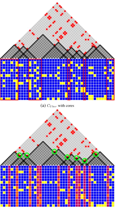
(a)CU berwith cores

(b)Flagging SNPs

Figure 2.2: This figure shows the CU ber intervals. (a) includes the cores, highlighted in red. (b) shows

(37)

I4 is aC(h)1,29cover,{I1, I3, I4, I6, I8}is a complete5-cover. We are particularly interested

in completek-covers, wherek is a reachable lower bound on the number of intervals for the

given SNP set.

In the following sections we provide an effective method for finding minimum-length

complete covers for a given SNP set. This establishesk as a tight lower bound. In general,

the k-cover for a given data set may not be unique. I provide several simple linear-time

algorithms that generate variousk-covers. In addition, we examine features which are

com-mon to allk-covers of a given data set. I then present a linear-time algorithm for finding a

cover composed entirely of maximal compatible intervals from CU ber, where |CU ber| ≥ k.

Finally, I present an algorithm for finding the k-cover with maximal overlap, the

Maximal-k-Cover (CM ax). The coverCM axis of particular interest since it leads to the construction of

a parsimonious set of perfect phylogeny trees where each incorporates maximal information

(i.e. the maximum number of SNPs per tree). Finally, I present an algorithm for finding

critical SNPs inS whose removal reduces|CM ax| fromk to k−1or smaller. This can be

accomplished using a number of tests proportional to|CU ber|rather thanm.

2.3.1 Constructing Phylogenetic Trees from Compatible Intervals

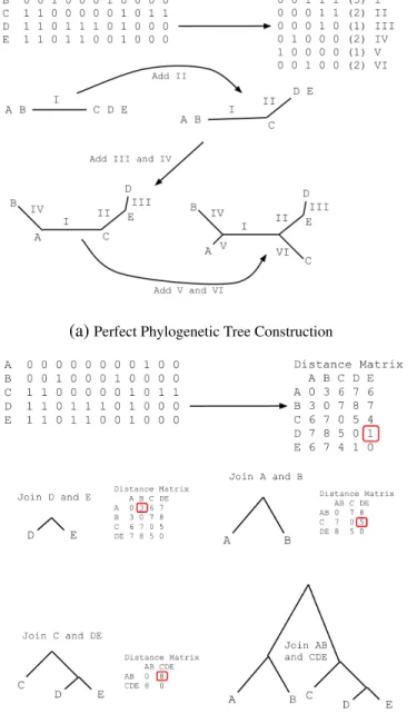
Every compatible interval admits an unambiguous phylogenetic tree, by definition [33].

While we are often concerned only with the haplotypes represented within an interval, we

also often interested in constructing the actual phylogenetic tree which represents the

varia-tion in an interval. This can be done simply and efficiently for binary haplotypes using the

method described in [33]. We wish to construct a perfect phylogeny tree in which each edge

represents an SDP in the compatible intervals. A rooted tree is constructed with the all-zero

haplotype at its root (there may be no actual representative of this haplotype). SDPs are

considered in decreasing order of the number of minority alleles present in all samples. For

(38)

A subtree is added to this leaf containing those samples with 1s (the minority allele).

Fig-ure 2.3a illustrates this tree construction procedFig-ure. When constructing local phylogenetic

trees in this way, the outgroup is most often unknown, so the resulting tree is considered

unrooted after it is fully constructed.

It is not trivial to construct a meaningful tree over genotypes unless they are phased and

the corresponding haplotypes admit a perfect phylogeny. However, when perfect phylogeny

trees are unreasonable or we wish to construct trees over intervals which do not strictly admit

a perfect phylogeny (in some circumstances, I consider the collection of several adjacent

intervals), I use other tree construction methods. The neighbor-joining method [69] allows

the efficient construction of parsimonious phylogenetic trees based on pairwise distances (in

our case, SNPs). Given a population of samples and pairwise distances between them, we

repeatedly merge the samples with the smallest distance (see Figure 2.3b). After merging two

samples, we remove them from further consideration and add a virtual sample with distances

to the remaining samples equal to the average distance from the two merged samples. These

”merges” represent the roots of successive subtrees until all samples are merged into the root.

This method accurately represents the relationships between samples when genotypes do not

admit a perfect phylogeny [69].

2.4 A Lower Bound

2.4.1 LR and RL Covers

We first define two non-overlapping covers, the Left-to-Right cover (C(h)LR), and the

Right-to-Left cover (C(h)RL). A simple greedy algorithm, LRScan (Algorithm 1), which has been

previously described in [89], findsC(h)LRover a set of haplotypes. It begins at the leftmost

SNP (s1), and either extends or terminates the current active interval as it considers each

(39)

(a)Perfect Phylogenetic Tree Construction

(b)Neighbor-Joining Tree Construction

(40)

already in the active interval. If four gametes occur between the SNP under consideration

and a previous SNP found in the interval, the active interval is closed, and a new interval

begins from the candidate, otherwise the SNP is added to the active interval. This continues

until the last SNP is reached, thus closing the final interval (see Figure 2.4a).

The run-time of LRScan depends on the number of SNPs,m, and the number of the FGTs

performed for each SNP. Since the maximum number of distinct compatible SNP patterns

that can be mutually compatible among n haplotypes is2n−3[77], the FGT requires only

O(n)operations per SNP, assuming a constant-time overhead for each FGT. Therefore, the

complexity for LRScan isO(mn), and thus is linear in the size of the data matrix.

Algorithm 1:C(h)LR=LRScan(SN P)

Input:SN P = [snp1, ..., snpm]: an array ofmmarkers

Output:C(h)LR : a list of intervals covering 1 tom

Variables: l: list of unique SNP patterns we have seen for the current interval

s: the start of the current interval

s←1

fori= 1tomdo ifsnpi ∈/ lthen

forj = 1to||l||do

iflj is not compatible withsnpithen

append toC(h)LR interval[s, i−1]

s←i l← ∅ break

addsnpi tol

append toC(h)LR interval[s, m]

returnC(h)LR

A similar greedy Right-to-Left scan algorithm (RLScan) generating C(h)RL can be

de-fined via straightforward modifications to (LRScan). LikewiseC(h)RL can be generated by

merely reversing the input sequence, applying LRScan, and adjusting the indices of the

re-sulting intervals, including their starting and ending positions. Note that a cover’s interval

(41)

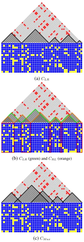
(a)CLR

(b)CLR(green) andCRL(orange)

(c)CM ax

Figure 2.4: This figure shows three covers. (a) depictsCLR created by the LRScan algorithm. (b) shows

CLR (in green) andCRL (in orange) together. The intersection of these two covers creates the set of cores

(42)

direction.

I define a similar notion over a set of genotypes. As described in Section 2.6, the only

difference is the manner in which the FGT is performed. We find an optimistic left-to-right

(C(g)LR) and right-to-left (C(g)RL) cover by closing an interval only when the subsequent

SNP will be definitely and unambiguously incompatible with a SNP in the interval (regardless

of the phasing chosen). Likewise, a pessimistic interval (C(p)LRandC(p)RL) is closed off if

there exists a phasing of the genotype set for which the next SNP will be incompatible with

SNPs already in the interval.

The run time of the pessimistic genotype scan is alsoO(mn). Like the haplotype case,

there is a limit on the number of distinct SNPs that can be compatible amongn genotypes

which is linear inn. So, the adjusted FGT requires onlyO(n)operations per SNP to

deter-mine if there exists any possible incompatibility.

The run time of the optimistic genotype scan is more complex. Eskin et al ([26])

pro-pose an algorithm withO(nm2₎_{complexity to determine if a single region admits a perfect}

phylogeny. I use a similar algorithm, adding SNPs incrementally. Since each interval is

bounded and scan proceeds linearly across the genome, this allows for anO(nm2₎_algorithm

to partition the entire genome.

2.4.2 Properties of

C

LR

and

C

RL

In this section I present properties of compatible intervals and provide proofs. My first

the-orem states that “The covers CLR and CRL have the same number of intervals k, and k

is the minimal number of intervals possible for any complete cover.” A second theorem

identifies certain core subintervals are common to all completek-covers of a given SNP set

(Figure 2.2a). These subintervals are the intersections of corresponding intervals fromCLR

andCRLwhich I have called cores (Figure 2.4b). This implies that ak-cover must containk

(43)

any interval that does not contain an entire core is not part of any completek-cover and the

second is that theith core is only contained within theith interval of anyk-cover. Cores have

several interesting properties worth noting. All SNPs in a core are compatible because each

core is an intersection of two compatible regions. Adjacent cores must contain at least one

pair of incompatible SNPs.

LEMMA 1. Anyc-interval cover covering the range[1, ec], withec≤m, satisfiesec≤eLc,

whereeL

c is the endpoint of thecthinterval ofCLR over the same sequence.

PROOF. By induction, a single-interval cover must end at, or short of, eL

1 (an overage

would indicate LRScan closed the interval prematurely). Assume that the Lemma holds for

ani-interval cover, thus ei ≤ eLi. This implies for any(i+ 1)-interval cover bi+1 ≤ bLi+1.

We now proveei+1 ≤eLi+1. Since there exists a SNP,s, in the(i+ 1)th interval ofCLR(i.e.

within[bL_i₊₁, eL_i₊₁]) wheresis incompatible withs_eL

i+1+1,[bi+1, ei+1]cannot be a compatible

interval ifei+1 > eLi+1. Therefore, we haveei+1 ≤eLi+1.

A symmetric Lemma forCRLstates that anyC-interval cover covering the range[b1, m],

withb1 ≥ 1, satisfies bc ≥ bRc, wherebRc is the start of thecth interval ofCRL over the same

sequence.

THEOREM 1. The coversCLR andCRLhave the same number of intervalsk, andk is the

minimal number of intervals possible for any complete cover.

PROOF. Assume kCLRk = i. According to Lemma 1, for any c-interval cover, C, with

c < iand starting from the left-most SNP, the end of the cover’s rangeec ≤ bLc < bLi =m.

Therefore,C cannot be a complete cover if kCk < kCLRk, implying that a complete cover

must have at leastkCLRkintervals. A similar conclusion can be drawn forkCRLkusing the

symmetric version of Lemma 1. Therefore, we have kCLRk = kCRLk = k, and k is the

(44)

LEMMA 2. For alli= 1. . . k,Corei 6=∅.

PROOF. By induction. Assume CLR = {I1L, . . . , IkL}, and CRL = {I1R, . . . , IkR}. By

definitionCorei is[bLi, eiR]; therefore, it is sufficient to prove bLi ≤ eRi . This is trivially the

case fori = 1;bL

1 ≤ eR1. Assume thatbLi ≤eRi holds fori, we now prove it holds for i+ 1.

From bL

i ≤ eRi , we know bLi < bRi+1. If biL+1 ≤ eRi+1 does not hold, implying eRi+1 ≤ eLi ,

then we knowI_iL ⊃ I_iR₊₁, and SNP s_eR i (∈ I

L

i )must be compatible with all SNPs in IiR+1.

Figure 2.5b illustrates this proof. s_eR

i is outside and adjacent to I

R

i+1. By definition of the

Right-to-Left cover, SNP s_eR

i must be incompatible with at least one SNP in I

R

i+1, which

results in a contradiction.

THEOREM 2. For any completek-coverC1,m={I1, . . . , Ik}, theith interval contains the

entire ith core: Corei ∩ Ii = Corei, and, it does not contain any part of another core

Corej∩Ii =φ,1≤j ≤k, j 6=i.

PROOF. Since Corei = [bLi, eRi ], to prove the ith interval Ii = [bi, ei] contains Corei,

it is sufficient to prove bi ≤ bLi and ei ≥ eRi . Since {I1, . . . , Ii−1} is an (i −1)-cover

covering the range[1, ei−1]starting from the leftmost SNP, according to Lemma 1, we have

ei−1 ≤eLi−1, which meansbi ≤bLi . Similarly, we can proveei ≥eRi (see Fig. 2.5c). To prove

Corej ∩Ii = ∅ for any other coreCorej, it is sufficient to prove ei < bLi+1 and bi > eRi−1.

Since{I1, . . . , Ii} is an i-cover covering the range[1, ei], according to Lemma 1, we have

ei ≤eLi < bLi+1. Similarly, we can provebi > eRi−1.

Stated formally, Corei = IiL ∩ IiR. According to Lemma 1, eRi ≤ eLi and bLi ≥ bRi

(Figure 2.5a), therefore Corei = [bLi, eRi ]. Theorem 2 states, “For any complete k-cover,

C{1, m} = {I1, . . . , Ik}, theith interval contains the entire ith core: Corei∩Ii = Corei,

and, it does not contain any part of another core Corej ∩Ii = Φ,1 ≤ j ≤ k, j 6= i”.

This is due to the interleaving of the non-overlapping intervals of CLR and CRL. Corei

is necessarily compatible with both IL

i and IiR and cannot be extended beyond the outside

(45)

PROPERTY 1. All SNPs in a core are compatible, since each core is an intersection of two

compatible intervals

PROPERTY 2. Adjacent cores must contain at least one pair of incompatible SNPs

PROOF. This can be demonstrated by contradiction. Assume that two adjacent cores,corei

andcorei+1, are compatible. By definition,corei = [bLi , eRi ]. Since corei ⊆ IiL = [bLi, eLi],

corei is compatible with [eRi + 1, eLi ]. Similarly, corei+1 is compatible with [eRi + 1, eLi].

Therefore,corei∪[eRi + 1, eLi]∪corei+1 = [bLi , eRi+1]is a compatible interval containing both

cores and contradicting Theorem 2 (Fig. 2.5d).

2.5 Max-

k

Interval Set

First we introduce UberScan, which generates the set of all the maximal compatible intervals,

CU ber. UberScan, shown in Algorithm 2, is similar to the LRScan. Whenever a compatible

interval ends at SNPsi, instead of starting the next interval from si + 1 as LRScan does,

UberScan finds the nearest SNP sj(j < i + 1) that is incompatible with si + 1, and the

following SNP, sj + 1, begins the next interval. Note that si + 1 is a flagging SNP of the

previous maximal compatible interval andsj is a flagging SNP of the next maximal

compat-ible interval. UberScan is a simple modification of LRScan with added bookkeeping to track

of the index of the last occurrence of each unique SNP pattern. Recall that the maximum

number of distinct SNP patterns within a compatible interval is2n−3, orO(n). An analysis similar to that of LRScan shows that UberScan also takesO(mn)time. UberScan generates

CU ber, containing all maximal intervals of S, and generally, |CU ber| k. CU ber contains

all candidates for the Maximal-k-cover,CM ax, since a cover with maximal overlap must be

(46)

(a)Shows the definition of core (Corei=IiL∩I R i )

(b)Illustration of the proof for Lemma 2

(c)Illustration of the proof for Theorem 2

(d)Illustration of the proof for Property 2

(47)

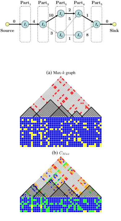
(a)Max-kgraph

(b)CM ax

(c)C(g)M ax

Figure 2.6:(a) shows thek-partite graph used to findCM axfor the running example. The node represents the

interval, and the edge connects intervals which overlap, with weight representing the number of shared SNPs. The longest path (bold) is computed from source to sink which isCM ax. It contains intervalsI1,I3,I5,I6, and I8fromCU ber, with a total overlap of 17. (b) is the Maximum-k-cover of the set of haplotypes,C(h)M ax. (c)

(48)

Algorithm 2:CU ber=UberScan(SN P)

Input:SN P = [snp1, ..., snpm]: an array ofmmarkers

Output:CU ber : a list of intervals covering 1 tom

Variables: l: sorted list of (position, SNP) tuples for the SNPs we have seen for the current interval

s: the start of the current interval

s←1

fori= 1tomdo

forj =||l||downto1do

iflj is not compatible withsnpithen

append toCU ber interval[s, i−1]

s←ljposition + 1

removel1tolj froml

break

appendsnpitol

append toCU ber interval[s, m]

returnCU ber

2.5.1 Finding the Maximal-k-cover

A Maximal-k-cover, CM ax, is of particular interest as it covers the entire SNP set using the

fewest,k, maximal intervals. While,CM ax is not necessarily unique, alternate solutions are

generally similar. Next we provide a fast graph algorithm to compute all Maximal-k-covers.

We consider only those maximal intervals inCU ber that entirely enclose a single core and

no part of a second core. According to Theorem 2, these intervals are the candidates for

Maximal-k-covers. Next, we organize the candidates into k groups according to the core

it contains. Each core is contained within at least one maximal interval, thus, no group is

empty. We then examine the overlap between groups. A candidate interval in group ican

only overlap candidates from groupsi−1or i+ 1, because, if any two candidates enclose non-adjacent cores (say Corex and Corey), at least one of them contains part of the core

betweenCorexandCorey, contradicting Theorem 2.

The Maximal-k-cover problem is solved by recasting it as finding the longest path in a

(49)

to a node and each group as a part, with particontaining all the candidates coveringCorei.

An edge connects nodes corresponding to overlapping candidates. Each edge’s weight is the

amount of overlap between the two intervals. The edge is directed towards the candidate that

contains the next core in the sequence. Because intervals only overlap adjacent groups, edges

only exist between adjacent parts. A source is added with edges to all nodes in part1and a

sink with edges from all the nodes in part k; both types of edges have weight0. Finding a

CM ax solution corresponds to finding the longest path in this directed graph withk+ 1edges

from source to sink. Note that the greedy approach of taking the largest interval that encloses

each core does not always yield a correct answer, as shown in the fourth core of our running

example (compare Figure 2.2a and Figure 2.4c).

The problem is a single-source shortest path problem for a weighted directed acyclic

graph (DAG), except that we search for longest path (maximizing instead of minimizing the

sum of weight on the path) with a constraint on the number of steps. The constraint can be

ignored since all edges lead from one part to the next, thus any path from source to sink will

havek+ 1steps. The problem can be solved using dynamic programming and requires only

Θ(|V|+|E|)time, whereV is the set of nodes, andEis the set of edges [15].

2.5.2 Critical SNPs

A critical SNP is any SNP whose removal reducesk, the minimum number of intervals

re-quired to cover the given SNP set. To check whether a SNP is critical, one could simply

remove each SNP and recalculatekby either a LRScan or an RLScan. This naive approach

requiresmscans, and takes O(nm2₎_{time. However, it is unnecessary to test every SNP. In}

fact, only flagging SNPs of maximal compatible intervals need to be considered. A flagging

SNP bounds an interval on one side and prevents the interval from growing toward an

adja-cent interval on that side, therefore a flagging SNP must be removed to allow any interval to

(50)

THEOREM 3. Critical SNPs are flagging SNPs ofCU berintervals.

PROOF. Consider two adjacent maximal compatible intervals,I_iU ber andI_iU ber₊₁ . Their

flag-ging SNPss_eU ber

i +1 andsbU beri+1 −1 must be incompatible (see Fig. 2.2b for an example). This

incompatibility makes it infeasible for eU ber

i to be larger and bU beri+1 to be smaller. Without

removing at least one of these two flagging SNPs, it is impossible for either of these two

in-tervals to grow towards each other. SinceCM ax ⊆CU ber, a necessary condition of reduction

inkis that at least one interval inCU bergrows in size. Therefore, being a flagging SNP is a

necessary condition for being a critical SNP.

Since each maximal compatible interval has two flagging SNPs, one on each side of the

interval, the total number of flagging SNPs isO(|CU ber|). The running-time for computing

critical SNPs isO(nm|CU ber|).

2.6 Genotypes

Determining four-gamete compatibility and compatible intervals over unphased genotype

data is ambiguous in that there are many possible interpretations (phasings) of a set of

geno-types as haplogeno-types. I define two approaches for determining compatibility among genogeno-types

without explicitly phasing. The optimistic method determines intervals for which there might

exist a phasing such that the interval is four-gamete compatible. The pessimistic method

de-termines intervals by choosing a phasing which introduces the maximum possible

incompat-ibility.

I compared the haplotype and genotype intervals on three data sets. First, I created

simu-lated genotype data using a simple infinite-sites model of mutation with cross-over

recombi-nation - this served as a data source devoid of confounding factors such as experimental error

and homoplasy. Second, I used real data from F1 crosses between isogenic mouse strains.

(51)

2.6.1 Relating Genotype and Haplotype Covers

In simulated data, one can explore relationships between the compatible intervals of

geno-types and the compatible intervals of their “source” haplogeno-types. These haplotyeps can be

used as ground truth for the corresponding set of genotypes. The number of intervals in an

optimistic genotype cover,||C(g)LR||, is less than or equal to the number of ground truth

in-tervals (Theorem 4) and the size of the pessimistic genotype cover,||C(p)LR||, is greater than

or equal to the number of ground truth intervals (Theorem 5). Thus, the number of intervals

in an optimistic and pessimistic genotype scan are lower and upper bounds, respectively, on

the true number of intervals.

THEOREM 4. kC(g)LRk ≤ kC(h)LRk

PROOF. By contradiction. Assume C(h)LR exists such that kC(h)LRk < kC(g)LRk.

There must exist some incompatibility in Sg not in S. By definition, it must be

impossi-ble to phaseSgto makeS. Therefore,Smust not be a true phasing ofSg.

THEOREM 5. kC(h)LRk ≤ kC(p)LRk

PROOF. By contradiction. Assume C(h)LR exists such that kC(p)LRk < kC(h)LRk.

There must exist some incompatibility in S not in Sp. By definition, it must be

impossi-ble to phaseSto makeSp. Therefore,Sp must not be a true phasing ofS.

COROLLARY 1. kC(g)LRk ≤ kC(h)LRk ≤ kC(p)LRk

In Figure 2.7, ‘a’ represents the distribution of the set of all possible genotype “pairings”

of a fixed haplotype set into genotypes. The “ground truth”, or the number of intervals

required to form a cover using the source haplotypes, is 5. Notice that the covers resulting

from every optimistic genotype scan fall closer to the “ground truth” than those from every

(52)

Figure 2.7:The distribution of cover sizes for genotypes resulting from all pairings of a set of haplotypes. For ‘a’ distributions, data was simulated using the infinite sites model and recombination. The source haplotypes cover size (the “ground truth”) is represented by the solid black line. For ‘b’ distributions, a contrived haplotype set was made by phasing a pessimistic genotype result of ‘a’. The source haplotypes cover size is the dashed black line.

In contrast, ‘b’ represents the same plot for a contrived, non-biologically-based,

haplo-type data set. The distribution of the cover size of all genohaplo-types can be formed by pairings

of the haplotype set that achieves one of the pessimistic covers from ‘a’ (this can always be

achieved, as discussed in Section 2.6.2). Specifically, the “true” cover size for this contrived

set is 23. Notice that the distribution is different from the biology-based model. In

particu-lar, the optimistic and pessimistic distributions are closer together and the “ground truth” is

nearer the pessimistic estimations.

2.6.2 Achieving Genotype Covers by Phasing

In many circumstances, it is useful to determine if a particular genotype cover or interval set

is achievable by phasing. Pessimistic genotype covers can always be achieved (see

Algo-rithm 3). However, there does not always exist a phasing to accomplish a given optimistic

5127.pdf

Analysis and Visualization of Local Phylogenetic Structure

within Species

Abstract

Acknowledgments

Table of Contents

List of Figures

List of Tables

Chapter 1

Introduction

1.1

Phylogenetics

1.1.1

Thesis Statement

1.2

Genetic Structure and Inheritance

1.2.1

Genomic Nomenclature

1.2.2

Genetic Variation

1.3

Compatible Intervals

1.4

Imputation using Local Phylogeny

1.5

Visualization of genomic structure

1.6

Conclusions

Chapter 2

Compatible Intervals

2.1

Introduction

2.2

Related Work

2.3

Definitions

2.3.1

Constructing Phylogenetic Trees from Compatible Intervals

2.4

A Lower Bound

2.4.1

LR and RL Covers

2.4.2

Properties of

C

and

C

2.5

Max-

k

Interval Set

2.5.1

Finding the Maximal-k-cover

2.5.2

Critical SNPs

2.6

Genotypes

2.6.1

Relating Genotype and Haplotype Covers

2.6.2

Achieving Genotype Covers by Phasing