Challenges in the automated classification of variable stars in
large databases
MatthewGraham1,2,,AndrewDrake1,S. G.Djorgovski1,AshishMahabal1, andCiroDonalek1
1California Institute of Technology, Pasadena, CA 91125, USA
2National Optical Astronomy Observatory, 950 N. Cherry Ave, Tucson, AZ 85000, USA
Abstract.With ever-increasing numbers of astrophysical transient surveys, new facili-ties and archives of astronomical time series, time domain astronomy is emerging as a mainstream discipline. However, the sheer volume of data alone - hundreds of obser-vations for hundreds of millions of sources – necessitates advanced statistical and ma-chine learning methodologies for scientific discovery: characterization, categorization, and classification. Whilst these techniques are slowly entering the astronomer’s toolkit, their application to astronomical problems is not without its issues. In this paper, we will review some of the challenges posed by trying to identify variable stars in large data collections, including appropriate feature representations, dealing with uncertainties, es-tablishing ground truths, and simple discrete classes.
1 Introduction
Time domain astronomy is now entering a golden age with an ever-increasing number of new instru-ments and facilities dedicated to repeated observations of large swathes of sky every few nights or so. This is not just limited to optical astronomy but extends right across the electromagnetic spectrum from radio to gamma-ray wavelengths and now to even more exotic physical domains with the emer-gence of neutrino (IceCUBE) and gravitational wave (LIGO) observatories. Even though many of these are dedicated to looking for real-time transients (things changing significantly from past obser-vations, if any), they can quickly generate substantial archives of data. Systematic searches of these for particular types of astrophysical source or phenomena require new approaches and in recent years, there have been a number of studies attempting automated classification and outlier detection using machine learning-based techniques (see Table 1). Obviously, these are all with an eye to the next generation of synoptic sky surveys, e.g., Gaia ([1]), ZTF ([2]), and LSST ([3]), which will increase the amount of available data by several orders of magnitude and mandate such approaches.
These types of analyses are not necessarily straightforward, though, and can present a number of issues related to how time series are represented (characterization), what groupings are present (categorization), and how individual time series are assigned to these (classification). The challenges are not just technical but also sociological: the Astronomer’s Telegram1(ATels) is a popular
mech-anism for distributing transient alerts but 50% of optical surveys mentioned in them have no public
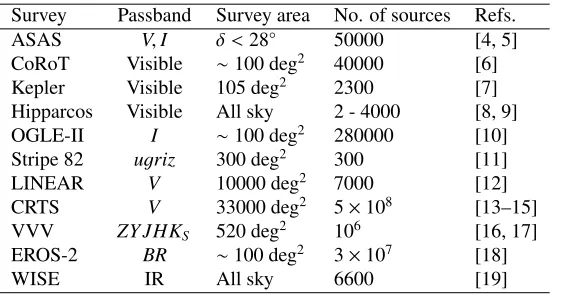
Table 1.A sample of automated classifications of various time domain surveys.
Survey Passband Survey area No. of sources Refs.
ASAS V,I δ <28◦ 50000 [4, 5]
CoRoT Visible ∼100 deg2 40000 [6] Kepler Visible 105 deg2 2300 [7] Hipparcos Visible All sky 2 - 4000 [8, 9] OGLE-II I ∼100 deg2 280000 [10]
Stripe 82 ugriz 300 deg2 300 [11]
LINEAR V 10000 deg2 7000 [12]
CRTS V 33000 deg2 5×10⁸ [13–15]
VVV ZY JHKS 520 deg2 106 [16, 17]
EROS-2 BR ∼100 deg2 3×10⁷ [18]
WISE IR All sky 6600 [19]
interface to their data holdings. These are also the larger surveys and one wonders how many smaller collections of astronomical observations and time series remain in the private domain. The success of automated classification relies on having access to the greatest amount of information and in this era of data-intensive astronomy, there is no lack of science exploration and discovery to do.
In the paper, we will review the mechanics of automated classification and associated issues that one attempting such an analysis should be cognizant of.
2 How to automatedly classify a data set
Most automated classification work follows the same basic workflow:
1. Astronomical time series are typically irregularly sampled, noisy, and gappy, and even within the same survey, they can vary in terms of number of observations, sampling, signal-to-noise ratios, etc., due to such factors as differing night-to-night observing conditions. These diff er-ences obviously make any analysis that is looking for similarities between these time series non-trivial, i.e., it is not just a case of computing a Euclidean distance between them. One way to handle irregular sampling is to interpolate the time series onto a regular temporal grid but this can also introduce additional errors and there may still be issues with missing values or large gaps. A more general approach is to convert the inhomogeneous raw data representation into a homogeneous one through the use of characterizing statistical features. For example, a set of 10,000 light curves, each consisting of between 10 and 50 observations with varying measurement errors can be replaced by a set of 10,000 measurements of median magnitude, in-terquartile range, and linear trend, say. This can also reduce the dimensionality of the problem: in the example, the raw parameter space is 50-dimensional whereas the feature parameter space has just three dimensions.
3. A classifier or set of classifiers are trained using the training set. Popular classifiers include ran-dom forest, support vector machines, and convolutional neural networks – the latter are a type of deep learning algorithm, which is regarded as the current state-of-the-art for image-based work.
Ensembleclassification methods, such as bagging, boosting, and stacking, use multiple classi-fiers to improve performance over individual classiclassi-fiers and generate more certain, precise, and accurate results.
4. A trained classifier is validated on atestdata set, which is independent from the training set, to assess its strength and utility. Validation using the training set will just result in an over-fitted classifier. Performance characteristics such as false negative and positive rates and their ratios to the true positive and negative rates, and summary measures, such as the F-score and Matthews correlation coefficient, are determined from the test set. For binary classifiers, ROC (receiver operating characteristic) curves show the classifier performance as its discrimination threshold is varied and allow optimal models to be selected. If a test data set is not available thencross validation can be employed: the training set is partitioned into subsets, which are iteratively used as training and validation sets. Performance characteristics are then calculated by averaging over the subsets.
5. The classifier is applied to the full data set. Population statistics can be determined for each class and outliers identified by poor class membership.
3 Characterizing astronomical time series
The challenge with time series characterization is to represent the time series in such a way that those which are interesting are easily distinguishable from the more run-of-the-mill ones. The most commonly-used discriminative features can be grouped in terms of the type of aspect they try to capture:
• Location: Mean, median
• Scale: Variance, median absolute deviation
• Variability: Stetson JHK indices, von Neumann index
• Morphology: Skew, kurtosis, interquartile region, cumulative sum index, ratio of magnitudes brighter/fainter than the mean
• Timescales: Lomb-Scargle derived period
• Trends: Phase folded slope percentiles, linear regression
• Model-based: Fourier amplitude ratios, phase differences, and amplitudes; Shapiro-Wilk normality test
The hope is that such features extracted from the data are informative and non-redundant, although there is a tendency in analyses to employ many features that all aim to broadly capture the same type of information. Unless the time series under analysis are densely sampled, the information content across such features will essentially be uniform.
3.1 Unstated assumptions
• Heteroskedasticity: Observations are taken on different nights with different seeing, weather con-ditions, instrumental settings, etc. It is therefore inappropriate to draw measurement errors on flux from the same underlying statistical distribution over the full temporal range of a time series (homoskedasticity), i.e.,σ(fi) ∼ N(0, σ2). Features involving errors are instead to be based on
σ(fi)∼ N(0, σ2i).
• Non-iid: Successive data points in a time series cannot be assumed to independently and identically distributed (iid) in the same way that spatial data might be. Temporal data is sequential and so there is an inherent dependence between observations. If the time difference between successive points is small enough then the error measurements can be correlated. Residuals will also carry some correlations, particularly if the time difference is small.
• Stationarity: The generating distribution of the time series and its statistical moments, i.e., mean, variance, etc., are assumed to be time independent. There are known astronomical sources for which this is not true: GRS 1915+215 has at least twenty variability states ([20]). Certain classes of time series models can deal with this, for example, generalized autoregressive conditional heteroskedas-tic (GARCH) models, which are used to describe financial time series, have a variance which is a stochastic function of time. There is also no requirement for nonstationary time series to be sta-tionary in any particular limit. Time series can be made weakly stasta-tionary locally by considering first-order differences instead of raw measurements.
• Ergodicity: It is assumed that the time average for one sequence is the same as the ensemble average:
ˆ
f(x)=lim
n→∞
1
n
n−1
k=0
fTkx.
Observations that are sufficiently far apart in time are assumed to be uncorrelated and new observa-tions therefore give extra information about the underlying process.
3.2 Not all features are equal
Feature relevanceis an aspect of machine learning which determines which features contribute the most information to a class label. Several automated classifications ([5, 8, 17, 21, 22]) have analyzed their results in this regard using a number of different techniques: for example, random forest has a feature importance measure or specific iterative approaches successively add/remove the most in-formative features based on some particular measure, such as class variance or mutual information. These analyses make it clear that most commonly-used features have little importance and are redun-dant, in part because many of them are highly correlated (all capturing the same information) and so do not offer much discriminative power between them. A practical upshot of this is that only a handful of relevant features need to be derived for a set of time series rather than a bucketful. Which features will, however, depend on the relative classes trying to be identified: there is (as yet) no silver bullet feature that distinguishes all possible classes.
3.3 The most important feature: period
0:01 0:1 1 10 100 1000 1e4 log10(period)(days)
0 1e4 2e4 3e4 4e4 5e4
F
requency
Figure 1.The distribution of 290,000 periods from the Variable Star Index (version 2017-03-20; [24]).
a sizable effect on classification: for example, [8] found a 22% misclassification error rate for non-eclipsing variable stars with a wrong period. Periodic feature routines also account for around 75% of computing time used in feature extraction ([21]) and so a wrong starting value can mean a waste of resources.
More generally, there is the issue of whether one quantity can capture the cyclical aspects of stellar variability. Kepler observations of RR Lyrae stars have shown that about 30% exhibit some form of Blazhko behavior – period and amplitude variation associated with mode switching – and there are also small amplitude cycle-to-cycle modulations in many RRabs. Close binary systems and long period variables are known to have cyclic period changes over multidecade baselines. Semi-regular variable stars commonly exhibit double periods and multiperiodicity. Finally, any variable source that can be described by a (C)ARMA (autoregressive moving average) process can expect to show quasi-periodicity (associated with peaks in the power spectrum).
Of the few hundred thousand periodic variable stars known, we typically have (sparse) temporal data for about a decade or two of coverage. For the majority of sources with periods on the order of a few days or shorter (see Fig. 1), this amounts to at least a couple of thousand cycles (though a much smaller fraction of these will actually have associated data). However, we have very limited information on how stable the measured periods are over these timescales. For decadal length surveys now under way/being planned, this could require a regular retraining of the classifier as class periods drift.
category (it uses a least-squares fit of a set of trigonometric functions to the data) as do wavelet-based methods. The latter category includes phase dispersion minimization (PDM; uses means), analysis of variance (AoV; use variance), Lafler-Kinman (uses string length), and entropy-based methods. Other methods employ rank ordering of the time series, Bayesian modeling, neural networks, Gaussian process regression with a periodic kernel, and convolutions.
To understand which period-finding algorithm might be optimal, we undertook an investigation ([23]) into the dependencies of the nine most popular algorithms on signal-to-noise ratio, number of observations, sampling strategy, and variable star class type. We were also interested in the perfor-mance characteristics of the algorithms since one that might take 30 s on average to find a period would require 100 CPU years to deal with a 100 million source data set. Our test data set consisted of 67,000 light curves with representation across the eruptive, pulsating, rotating, cataclysmic, and eclipsing classes of variable stars.
We found that no single algorithm was generally better than∼60% accurate across the full data set (we assumed that the ground truth was at most a few percent inaccurate – the quoted periods had all been verified by visual inspection by at least three of the authors). All methods are dependent on the quality of the time series and show a decline in period recovery with lower quality time series as a consequence of fewer observations, fainter magnitudes, and noisier data, and an increase in period recovery with higher source variability. The algorithms were stable with a minimum bin occupancy in the phase-folded space of 10 for a bin width ofΔφ=0.1. A bimodal observing strategy consisting of pairs (or more) of close-separated observations (shortΔt) per night and normal repeat visits (every few nights or so) was better than just regular single visits. The algorithms worked best with pulsating and eclipsing variable classes, perhaps unsurprisingly as these tend to have the most sinusoidal wave-forms. Lomb-Scargle (and its variants) was strongly effected by the “half-period issue”: for eclipsing binaries, the algorithm tends to return half the true period value. Finally, specific algorithms worked better irregular sampling, bright magnitudes (containing saturated values), or with performance
For a choice of single algorithm, the recommendation was AoV.
3.4 Are we using the best features
As mentioned above, a lot of the standard features used in the literature are correlated, e.g., variance, median absolute deviation, and interquartile range are all estimates of scale. They also focus on cap-turing morphological aspects of the time series for discriminative purposes - the aim is to create groups of time series that look similar. However, the shape of a time series does not necessarily correlate in any simple way with the underlying physical process(es) that generated it. An alternate approach is to draw on domain knowledge to define phenomenologically motivated features that might be able to group time series based on common physics. For example, chaotic processes can be quantified by the Lyapunov exponent, autocorrelation identified by the Durbin-Watson statistic, and nonlinearity by the Teraesvirta measure.
4 Which classifier?
Most individual classifiers will give broadly the same results for the same feature set in terms of performance characteristics such as precision and recall. The errors on the characteristics are typically at the few percent level, particularly for classifiers with a strong stochastic element, e.g., random forest, and so there really is no difference between a classifier that is 88% accurate and one that is 90% accurate. As with period finding algorithms, certain classifiers may have slight preferences for certain classes where the discriminating hyperplane has some particular form. The state of the art classifier is random forest (although see also support vector machines, Bayesian networks, and self-organizing maps). Better results can be obtained with an ensemble classifier which incorporates the relative strengths of each individual classifier and thus obtains better predictive performance than any of them (typically accuracy will go from 85-90% to 95-99%) . In general, there are two types of such ensemble methods: averaging methods, such as bagging where the combined (averaged) prediction of the independent constituent methods has reduced variance (random forest actually works along these lines with decision trees as the base classifier); and boosting methods, in which weak component methods are combined incrementally to create a strong method with reduced bias. There are also hierarchical ensemble methods where the class outputs of a base layer of classifiers are used as inputs to a secondary (or subsequent) layer(s).
4.1 Dealing with uncertainties
There are many sources of uncertainty: time series have observation errors in flux (and time, although we rarely consider these); regularization and imputation to deal with irregular sampling and missing values add interpolation uncertainties; and model parameters and hyperparameters have their own uncertainties. Feature representations do not traditionally deal with these (and alternate data repre-sentations will also introduce their own uncertainties). Probabilistic classifiers tend only to simulate the effect of observation errors through the choice of priors or parameter space coverage in training sets.
Ideally, though, a full probability density function should be given for any classification: for example, a source is not longer classed as an RR Lyrae or eclipsing binary but has a 62% change of being an RR Lyrae, a 28% change of being an eclipsing binary and a 10% chance of something else. Uncertainty quantification (UQ) formally considers this through both forward UQ with simulations and expansions methods and inverse UQ via Bayesian techniques.
4.2 A word about automated classification
4.3 Establishing ground truths
It can almost be guaranteed that the assumed ground truth will not be 100% correct and this has a number of consequences. The (automated) classifier will be mistrained and this will raise the false positive/false negative rates in data to which it is applied. It should be noted that a 1% misclassifica-tion rate is highly significant when dealing with large data sets, for example, containing 100 million sources.
Currently, there is a lack of a (comprehensive) community-agreed training set for stellar classifi-cation, particularly at fainter magnitudes (V >16). Compiled catalogs, such as the General Catalog of Variable Stars (GCVS), the Variable Star Index (VSX), or even SIMBAD, are known to be hetero-geneous and have varying inaccuracies in the class flags. The respective population sizes of different classes of objects within these catalogs is also biased towards specific classes, e.g., RR Lyrae and eclipsing binaries, rather than being representative of the true astrophysical populations. For example, MACC ([5]) has∼20% of sources as semiregular variables and∼20% as small amplitude red giants.
4.4 Class distinctions
The question of exactly how many classes there may in a data set is essentially unanswerable. It will always be dependent on the both the objective state of domain knowledge at the time of classification and subjective choices made by the domain scientist carrying out the classification. There can also be different levels of classification employed, particularly when using a hierarchical system: for example, according to [4] stellar variability may be regarded at a high level as intrinsic or extrinsic to the source in origin or at a lower level originating from eruptive, pulsating, rotating, cataclysmic, or eclipsing processes.
Most classification schemes assume mutually exclusive classes, e.g., a source is either a RR Lyrae or an eclipsing binary but not both.Fuzzyclustering employs overlapping class boundaries, described by membership functions, and so multiple class memberships are possible, Sources can thus be des-ignated as 80% RR Lyrae and 20% eclipsing binary, say. This treats class as much of a continuum quantity than a complete discrete one.
Unsupervised learning can determine clusters through different cluster paradigms: partitional, hierarchical, density-based, grid-based, correlation, spectral, gravitational, herd, etc. These all have different assumptions, for example, partitional clustering places all clusters on the same level rather than in a taxonomy, say, and density-based clustering will associate different classes with peaks in the density field of the characterizing feature space. It is also arguable whether classes associated with clusters from an algorithm are physically realistic: does division of a feature space naturally map to a structured view of domain knowledge?
An often overlooked possibility in classification is an “other” class which holds sources that do not fit well into any of the prescribed classes. 60% of objects in MACC [5] are in the “MISC” class and the most accurately classified sources in the CRTS periodic variable catalog ([13]) belong to the aperiodic noise class.
4.5 Extremes
However, there is no reason why the characterized variability of every type of astronomical source in the observable universe over a decadal baseline should follow a Gaussian distribution. For a generic heavy-tailed distribution, defined by
lim
x→∞P[|X|>x]x −α=λ,
λandαcannot be estimated from data and so the general statistical significance of a source known. A specific choice has to be made about the distribution, e.g., it is Cauchy or Weibull, for a numerical significance to be evaluated.
There is no formal statistical definition for an outlier but it can be shown that the presence of outliers has no connection with either the existence of heavy tails of an underlying distribution or with experimental errors ([28]). From a topological perspective, a significant outlier is also not necessarily related to an underdensity in any distribution but rather has high persistence over a range of scales and marginal connectivity to the general population.
5 Summary and future work
Automated classification is a necessity when working with large data sets; there are, however, a num-ber of caveats to be aware of. Astronomical time series need to be represented in terms of features but the choice of features is not simple and each feature comes with inherent (statistical) assumptions and dependencies. It needs to be understood how errors in these representations propagate through and combine with others in the classification process to the final class assignment, which should also have an error model associated with it rather than being categorical. The actual choice of classifica-tion algorithm is not necessarily as important as is sometimes made out but the choice of training set used with it is. The ground truth associated with it needs to be researched as it it reflects a particular set of assumptions. The available set of class assignments also needs to be looked at and the reality of them considered in terms of current domain knowledge. Finally, if one is interested in outliers, consideration must be given to what an outlier actually is.
These issues are not unsurmountable and the promise of automated classification is the generation of statistically significant samples of rare phenomena: a 100 million object data set will contain 10,000 examples of a 1 in 10,000 source and a hundred of a one-in-a-million. The challenge then becomes to understand these.
Acknowledgments: This work was supported in part by the NSF grants AST-1413600 and AST-1518308.
References
[1] Mignard, F., MmSAI,83, 918 (2012)
[2] Bellm, E., inThe Third Hot-wiring the Transient Universe Workshop, ed. P. R. Wozniak et al., p. 27 (2014)
[3] Ivezic, Z., et al.,arXiv:0805.2366(2011) [4] Eyer, L., & Blake, C., MNRAS,358, 30 (2005)
[5] Richards, J., Starr, D., Miller, A., Bloom, J., Butler, N., Brink, H., & Crellin-Quick, A., ApJS,
203, 32, (2012)
[6] Debosscher, J., Sarro, L.M., Lopez, M., et al., A&A,506, 1 (2009) [7] Blomme J., Debosscher, J., De Ridder, J., et al., ApJL,713, 204 (2010) [8] Dubath, P., Rimoldini, L., Süveges, M., et al., MNRAS,414, 2602 (2011) [9] Rimoldini, L., Dubath, P., Süveges, M., et al., MNRAS,427, 2917 (2013) [10] Sarro, L. M., Debosscher, J., Aerts, C., & Lopez, M., A&A,506, 535 (2009) [11] Süveges, M., Sesar, B., Varadi, M., et al., MNRAS,424, 2528 (2012) [12] Palaversa, L., Ivezic, Z., Eyer, L., et al., AJ,146, 101 (2013)
[13] Drake, A.J., Graham, M.J., Djorgovski, S.G., et al., ApJ,790, 3 (2014) [14] Torrealba, G., Catelan, M., Drake, A.J., et al., MNRAS,446, 2251 (2015) [15] Drake, A.J., Djorgovski, S.G., Catelan, M., et al., MNRAS, submitted (2017) [16] Catelan, M., Minniti, D., Lucas, P.W., et al.,arXiv:1310.1996(2013)
[17] Elorrieta, F., Eyheramendy, S., Jordan, A., et al., A&A,595, 11 (2016)
[18] Kim, D.-W., Protopapas, P., Bailer-Jones, C. A. L., Byun, Y.-I., Chang, S.-W., Marquette, J.-.B., & Shin, M.-S., A&A,566, 43 (2014)
[19] Masci, F., Hoffman, D., Grillmair, C., & Cutri, R., AJ,148, 21 (2014) [20] Hannikainen, D. C., et al., A&A,435, 995 (2005)
[21] Richards, J. W., Starr, D. L., Butler, N. R., Bloom, J. S., Brewer, J. M., Crellin-Quick, A., Higgins, J., Kennedy, R., & Riscahrd, M., ApJ,733, 10 (2011)
[22] D’Isanto, A., Cavuoti, S., Brescia, M., Donalek, C., Longo, G., Riccio, G., & Djorgovski, S. G., MNRAS,457, 3119 (2016)
[23] Graham, M. J., Drake, A. J., Djorgovski, S. G., Mahabal, A. A., Donalek, C., Duan, V., & Maker, A., MNRAS,434, 3423 (2013)
[24] Watson, C., Henden, A. A., & Price, A., SASS,25, 47 (2006)
[25] Huppenkothen, D., Heil, L. M., Hogg, D. W., & Mueller, A., MNRAS,466, 2634 (2017) [26] Soszynski, I., Udalski, A., Szymanski, M. K., et al., AcA,66, 131 (2016)
![Figure 1. The distribution of 290,000 periods from the Variable Star Index (version 2017-03-20; [24]).](https://thumb-us.123doks.com/thumbv2/123dok_us/8133347.1355505/5.482.102.374.82.303/figure-distribution-periods-variable-star-index-version.webp)
