Simulation-Based Joint Estimation of Body
Deformation and Elasticity Parameters for Medical
Image Analysis
Huai-Ping Lee
A dissertation submitted to the faculty of the University of North Carolina at Chapel Hill in partial fulfillment of the requirements for the degree of Doctor of Philosophy in the Department of Computer Science.
Chapel Hill 2012
Approved by: Ming C. Lin Mark Foskey Marc Niethammer Ed Chaney
c
2012 Huai-Ping Lee ALL RIGHTS RESERVED
Abstract
HUAI-PING LEE: Simulation-Based Joint Estimation of Body Deformation and Elasticity Parameters for Medical Image Analysis.
(Under the direction of Ming C. Lin.)
Elasticity parameter estimation is essential for generating accurate and controlled simulation results for computer animation and medical image analysis. However, finding the optimal parameters for a particular simulation often requires iterations of simulation, assessment, and adjustment and can become a tedious process. Elasticity values are especially important in medical image analysis, since cancerous tissues tend to be stiffer. Elastography is a popular type of method for finding stiffness values by reconstructing a dense displacement field from medical images taken during the application of forces or vibrations. These methods, however, are limited by the imaging modality and the force exertion or vibration actuation mechanisms, which can be complicated for deep-seated organs.
In this thesis, I present a novel method for reconstructing elasticity parameters with-out requiring a dense displacement field or a force exertion device. The method makes use of natural deformations within the patient and relies on surface information from segmented images taken on different days. The elasticity value of the target organ and boundary forces acting on surrounding organs are optimized with an iterative optimizer, within which the deformation is always generated by a physically-based simulator. Ex-perimental results on real patient data are presented to show the positive correlation between recovered elasticity values and clinical prostate cancer stages.
Dedication
To my parents and Chen-Yi.
Acknowledgments
The past six years at UNC-Chapel Hill has been an exciting journey, and I was very lucky to be able to work with the best minds in the world. First and foremost, I would like to thank my advisor, Prof. Ming Lin, who guided and encouraged me through the PhD process. I also thank my committee members; Prof. Mark Foskey, who led me into the world of medical imaging and paper writing, and had been co-advising me until he took his talent to Morphormics (now part of Accuray); Prof. Marc Niethammer, who kept my math and logic as clean as possible; Prof. Ed Chaney, who gave me a lot of insights in cancer treatment and staging; and Prof. Ron Alterovitz, who provided discussions and comments about medical simulations.
I thank previous and present members of GAMMA group and MIDAG for discussion and feedback on my work, in particular, Dr. Vivek Kwatra, Rahul Narain, Yero Yeh, Prof. Stephen Pizer, Prof. Steve Marron, Josh Levy, Rohit Saboo, and Chen-Rui Chou. My presentations would not have the same quality without the feedback and criticism from group meetings and discussions, especially from Sean Curtis. I also thank people at Department of Radiation Oncology, especially Sue Xu, Gregg Tracton, Graham Gash, and Dr. Ron Chen, for providing prostate patient data and technical support.
It would be impossible for me to study abroad without support from my parents, who put my education above everything else. I am also grateful to my friends in Taiwan, in Chapel Hill, and around the world, for sharing laughs and keeping me motivated throughout the years.
Table of Contents
List of Tables . . . x
List of Figures . . . xii
1 Introduction . . . 1
1.1 Elastography . . . 4
1.2 Deformable Registration . . . 5
1.3 Parameter Estimation in Computer Graphics . . . 6
1.4 Joint Estimation of Deformation and Elasticity Parameters . . . 6
1.5 Thesis Statement . . . 8
1.6 Main Results . . . 9
1.6.1 Elasticity Estimation for Noninvasive Cancer Stage Assessment . 9 1.6.2 Applications in Medical Image Analysis for Radiotherapy . . . 11
1.6.3 Application in Physically-Based Animation . . . 13
1.6.4 Acceleration of Optimization Framework Using Reduced-Dimension Finite Element Modeling . . . 14
1.7 Organization . . . 16
2 Previous Work . . . 18
2.1 Elastography . . . 18
2.1.1 Displacement Field Estimation . . . 19
2.1.2 Inverse Modeling of Elastic Deformation . . . 20
2.1.3 Other Elasticity Estimation Methods . . . 20
2.2 Deformable Image Registration . . . 21
2.2.1 Image-Based Methods . . . 22
2.2.2 Landmark-Based Methods . . . 23
2.2.3 Simulation-Based Methods . . . 23
2.3 Parameter Estimation in Computer Graphics . . . 24
2.3.1 Directing Simulations . . . 24
2.3.2 Estimating Material Properties . . . 25
3 Simulation-Based Joint Estimation of Deformation and Elasticity Pa-rameters . . . 26
3.1 Introduction . . . 27
3.2 Method . . . 30
3.2.1 Linear Elasticity Model and Finite Element Modeling . . . 30
3.2.2 Sensitivity Study . . . 32
3.2.3 Distance-Based Objective Function . . . 34
3.2.4 Numerical Optimization . . . 36
3.2.5 Initial Guess of Parameters . . . 37
3.3 Experiments . . . 38
3.3.1 Synthetic Scene with Multiple Organs . . . 40
3.3.2 Noninvasive Assessment of Prostate Cancer Stage . . . 42
3.3.3 Study: Inhomogeneous Materials . . . 48
3.3.4 Application: Registration of Segmented CT Images . . . 51
3.3.5 Extension: Nonlinear FEM . . . 52
3.4 Conclusion and Future Work . . . 54
4 Treatment Image Estimation Based on Marker Locations for Dose Calculation . . . 58
4.2 Deformation Estimation Based on M-reps . . . 62
4.2.1 M-reps . . . 62
4.2.2 Rotational Flows and Deformation Field Generation . . . 64
4.3 Simulation-Based Estimation of Deformation . . . 65
4.3.1 Finite Element Modeling . . . 65
4.3.2 Optimization . . . 66
4.4 Dose Calculation . . . 67
4.5 Experiments . . . 68
4.5.1 Comparison of Organ Surfaces . . . 68
4.5.2 Comparison of Calculated Dose . . . 69
4.6 Summary . . . 71
5 Fast Optimization-Based Elasticity Parameter Estimation Using Re-duced Models . . . 76
5.1 Introduction . . . 77
5.2 Previous Work . . . 79
5.3 Method . . . 83
5.3.1 Optimization-Based Framework with Finite Element Modeling . 84 5.3.2 Acceleration using Reduced-Dimension Modeling . . . 85
5.4 Implementation and Results . . . 88
5.4.1 Physically-Based 2D Shape Deformation . . . 88
5.4.2 3D Elastography using Reduced Modeling . . . 89
5.5 Conclusion . . . 95
6 Discussion . . . 97
6.1 Summary of Results . . . 97
6.2 Future Work . . . 99
List of Tables
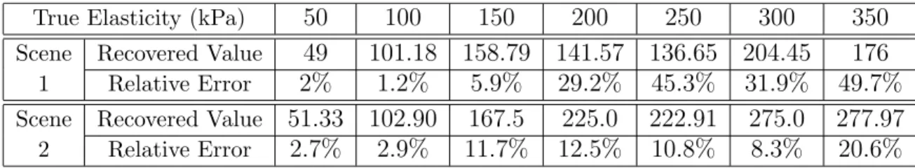
3.1 Error in recovered modulus of elasticity in two synthetic multi-organ scenes; note that the error becomes much larger for elasticity values greater than 150 kPa. . . 41 3.2 Average and standard deviation of elasticity values for the prostate
re-covered from the patient data sets; the last column is the clinical cancer staging for the tumor for each patient. . . 45 3.3 Definition of clinical T-stages for prostate cancer . . . 46 3.4 The recovered elasticity values for the prostate as a homogeneous
mate-rial, when the organ contains a synthetic tumor of different sizes and a normal tissue; elasticity values are set to 100 kPa for the tumor and 50 kPa for normal prostate tissue. . . 48 3.5 Average error in landmark positions (distance in cm) inside the prostate,
computed with the Demons method and my method; t-tests show that my method performs statistically significantly better in three of the five data sets. (If Bonferroni correction is used, my method is significantly better only for Patient 3.) . . . 52 3.6 Error in recovered nonlinear modulus of elasticity in two synthetic
multi-organ scenes. . . 53 3.7 Error in recovered nonlinear modulus of elasticity in two synthetic
multi-organ scenes where the elasticity of surrounding tissue is doubled (20 kPa) when generating the synthetic data. The surrounding tissue elasticity is still set to 10 kPa in the optimization process, and I expect to see recovered values for the prostate to be half of the true values. . . 54 3.8 Average and standard deviation of elasticity values for the prostate
re-covered from the patient data sets using nonlinear FEM; the last column is the clinical cancer staging for the tumor for each patient. . . 55
4.1 Average errors in prostate surface and volume for the four patient data sets. The surface error is measured with average distance between two sets of sample points (D), and the volume overlap is measured with the ratio of intersection and union of the two volumes (IntersectionUnion ). . . 69
4.2 Comparison of equivalent uniform dose of the dose-volume histograms for the prostate for the four patient data sets; the errors resulted from estimated images (using m-rep and FE simulation) are relative to the values given by the IGRT (using real treatment images). Each patient is experimented on using five target volume margins around the prostate. . 73 4.3 Comparison of equivalent uniform dose of the dose-volume histograms for
the anterior rectal wall for the four patient data sets; the errors resulted from estimated images (using m-rep and FE simulation) are relative to the values given by the IGRT (using real treatment images). Each patient is experimented on using five target volume margins around the prostate. 74
List of Figures
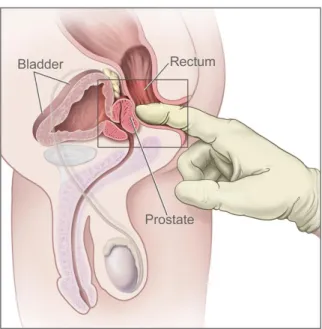
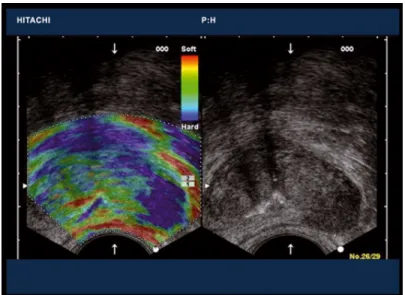
1.1 Digital rectal exam (DRE); the doctor inserts a gloved, lubricated finger into the rectum to feel and check the prostate. Courtesy of National Cancer Institute. . . 2 1.2 An example elastography result for the prostate using a rectal probe. Left:
overlaid colormap represents recovered elasticity. Right: corresponding ultrasound image. Courtesy of Hitachi Medical Systems. . . 3 1.3 Example 2D shape deformations showing different results with different
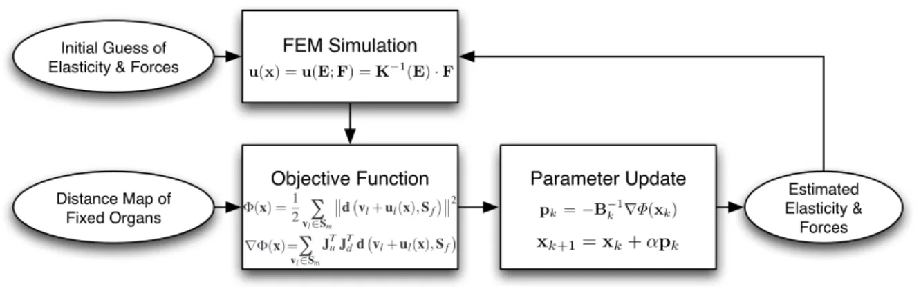
Poisson’s ratiosν; the boundary conditions are the same for both sets of objects (the gravity). . . 7 1.4 Overview of the optimization framework; the simulation parameters are
updated according to the current error in deformed surface and fed into the simulator for the next iteration. . . 7 1.5 A typical scene of the male pelvis region: the movement of the bladder and
rectum deforms the prostate. Left: a 3D rendering of the organ surfaces; the white surface represents the target surface of the prostate. Right: a slice of a CT image of the area; the red contour shows the segmentations of the reference image, and the blue contour shows the prostate in the target image. . . 9 1.6 Box plot showing the range of recovered elasticity values (Y axis) for
patients within each cancer stage (X axis), where the top and bottom of the boxes show the 25th and 75th quartiles, and top and bottom lines show the maximum and minimum values; the data shows significant positive correlation between the two values (the estimated p-value is 0.024 using Spearman’s rank correlation). . . 10 1.7 A typical setting of the Calypso system. Left: three transponders are
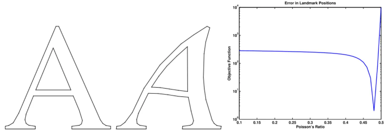
implanted into the prostate to provide localization; courtesy of Calypso. Right: a CT image slice showing the prostate and two of the transponders. 12 1.8 The initial shape (left), target shape (middle), and the plot of error versus
Poisson’s ratio (right), where the error is based on the distance between corresponding vertices; the recovered value is 0.48 (ground truth is 0.49). 14 1.9 Visualization of the first two principal components (reduced bases) found
by the statistical training of surface deformation. . . 15
1.10 The trade-off between speed and accuracy is achieved by using a different number of bases for representing nodal displacements in the FE model. . 16
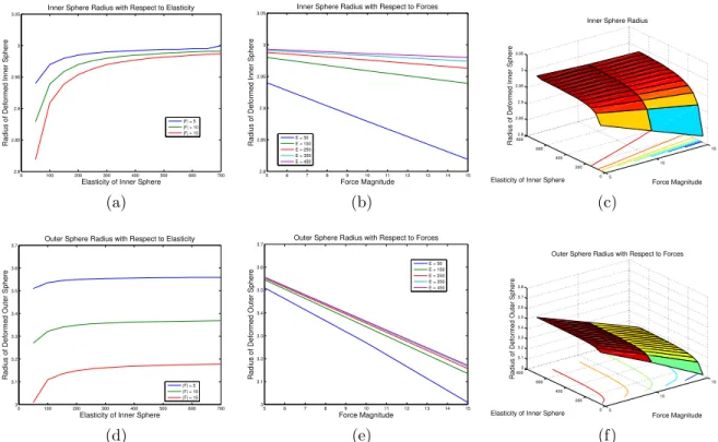
3.1 A sliced view of the synthetic scene, which consists of two concentric spheres; the inner (red) and outer (green) regions have different stiffness values (blue triangles represent outer surface, which is considered part of the green region). . . 32 3.2 The plots of the radius of the inner sphere (in cm) after deformation:
(a) inner radius versus elasticity value (in kPa) of the inner region; (b) inner radius versus magnitude of forces (in N) acting on the outer surface; (c) inner radius (z-coordinate) versus elasticity and force magnitude with isocontours of inner radius onxy-plane; (d) outer radius versus elasticity; (e) outer radius versus magnitude of forces; (f) outer radius (z-coordinate) versus elasticity and force magnitude with isocontours of outer radius on
xy-plane. The radii before deformation are 3 cm and 3.75 cm for two spheres, respectively, and the elasticity for the outer region is 10 kPa. The Poisson’s ratios are fixed to 0.40 and 0.35 for the two regions, respectively. 33 3.3 Input to my algorithm: (a) a sliced view of the tetrahedral model of the
moving image (light-blue triangles represent surfaces, not FEM regions; bladder and rectum are hollow); (b) a slice of the distance map of the prostate surface in the reference image. . . 36 3.4 Plot of Φ and E (in kPa) with several sample values for finding an
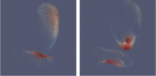
ini-tial guess of elasticity value in a synthetic multi-organ scene. The plot suggests that the best initial guess is 50 kPa. . . 38 3.5 The moving surfaces and ground-truth boundary conditions in the two
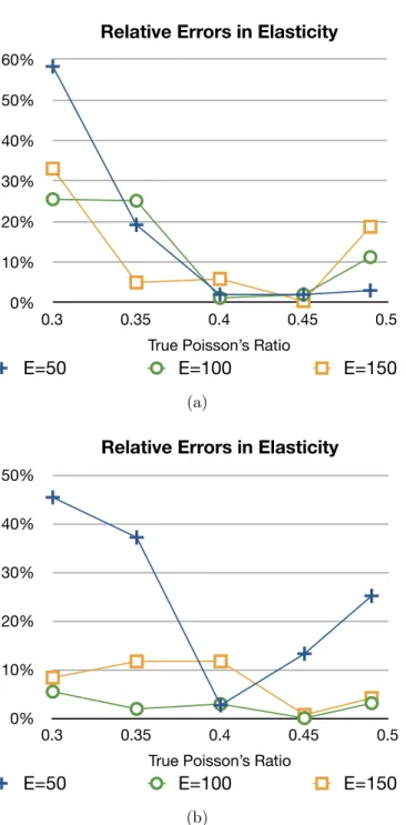
synthetic multi-organ scenes: the arrows shows Dirichlet boundary con-ditions applied to surfaces of bladder and rectum; the scaling of arrows are according to the magnitude of displacements. . . 41 3.6 Plots of relative errors in recovered elasticity vs. different Poisson’s ratios
for the prostate (0.3, 0.35, 0.4, 0.45, and 0.49) used for generating the synthetic surface data; each plot shows the result from one test scene, and each curve represents a true elasticity value (50, 100, and 150 kPa) used in the synthetic case. During the optimization process, the assumed Poisson’s ratio is always fixed to 0.4. . . 43 3.7 Histogram of distances between the pairs of corresponding reference and
3.8 Convergence graphs (plot of Φ andk∇Φk versus iteration number) for a pair of CT image data: (left) convergence of the external forces; (right) convergence of the elasticity. . . 45 3.9 Box plot of average recovered elasticity value and cancer T stage for each
patient data set shown in Table 3.2. . . 47 3.10 A sliced view of the tetrahedral mesh with a tumor (yellow) embedded
in the prostate (red); the mesh is used to generate the synthetic target surface, while the prostate is still considered homogeneous in the opti-mization process. . . 49 3.11 Close-up view of the surfaces before (left) and after (right) deformation;
the transparent white surface shown is the target surface of the prostate. Notice how the prostate surface move towards the white surface. Bladder and rectum surfaces are those with external forces applied. . . 49 3.12 Registration results for a pair of test images: (a) axial and sagittal views
of the moving image, and a 4x4 checkerboard comparison with the plan-ning image, before registration; (b) the two views of the registered image, along with a checkerboard comparison with the planning image; super-imposed by segmentations of the reference image, shown in red, and the segmentation of the prostate in the daily image, shown in blue; notice that the image deforms towards the red contours. . . 50 3.13 Box plot of average recovered nonlinear elasticity value and cancer T stage
for each patient data set shown in Table 3.8. . . 55
4.1 The Calypso System; three electromagnetic transponders are implanted in the prostate (left) prior to the treatment planning and are tracked in real time during each treatment fraction to provide localization (right). Courtesy of Calypso. . . 60 4.2 A simple 3×4 m-rep. A single shape is represented by the locations of
the hubs and the lengths and directions of the spokes. The boundary of the object (not shown) passes through the ends of the spokes. . . 63 4.3 3D rotational flow between two oriented points (x0,E0) and (x1,E1) lies
on a helix whose axis is the rotation axis between E0 and E1. Courtesy
of Levy et al. [2008]. . . 64 4.4 A finite element mesh used for estimating the deformation using the
simulation-based approach. The red elements represent the prostate. . . 66
4.5 Two examples of nodal displacement field resulted from the simulation-based optimization framework; the white transparent surface is the prostate.
. . . 67 4.6 Axial (left), coronal (center), and sagittal (right) views of an example
m-rep comparison; blue contour: m-m-rep fitted to Calypso marker locations during the treatment fraction; green contour: surface deformed by the simulation-based scheme; red contour: m-rep created with real treatment image; the green crosshairs show the Calypso origin, which also serves as the isocenter of the treatment plan; (a, c) CT images estimated using fitted m-reps and the simulation-based scheme, respectively; (b, d) 4×4 checkerboard images comparing (a) and (c) to the real treatment image, respectively. . . 70 4.7 Differential (a) and cumulative (b) dose-volume histograms for the prostate
(left) and anterior rectal wall (right); blue lines represent results with real treatment images, green lines represent results with images estimated us-ing m-rep fittus-ing, and red lines represent results with images estimated using FE simulation. . . 72
5.1 Flow chart of the optimization loop; the displacement field generated by the simulator is used in the objective function for the optimizer to update the parameters; updated parameters are fed back into the simulator, and so on. . . 83 5.2 The process of generating the the node correspondence and example
de-formations for one source surface; this procedure is repeated for multiple source meshes, and the resulting reduced basis can be applied to other FE meshes using the same node correspondence procedure. . . 88 5.3 Example 2D shape deformations showing different results with different
Poisson’s ratiosν(each column results from the same first-type boundary conditions); top: ν = 0.1; middle: ν = 0.49; bottom: comparison by overlaying the two results. . . 89 5.4 Flow chart of Poisson’s ratio estimation given source and target 2D shapes;
an FE model is built according to the source shape, and the distance be-tween the deformed source shape and the target shape is minimized. The red cross marks the nodes with boundary conditions applied. . . 90 5.5 Test of accuracy of the recovered Poisson’s ratiosν; the four target shapes
are generated using four differentν values; for each subfigure, on the left is the target shape, and on the right is the plot of surface errors versus ν
5.6 The tetrahedral mesh of the bladder-prostate-rectum area (left) and a close-up view of the three organs (right), where the white surface is the target prostate surface. . . 92 5.7 The first two principal components (visualized as nodal displacements on
bladder and rectum surfaces) resulted from a PCA using 108 example deformations. . . 93 5.8 The number of reduced basis vectors provides a means of trade-off between
optimizer performance and accuracy of recovered elasticity values; the error (blue) decreases and the number of optimization iterations (green) increases with the number of basis vectors used. The slight increase in error with 139 basis vectors is likely the result of optimizer sticking to a local minimum. . . 94
Chapter 1
Introduction
Figure 1.1: Digital rectal exam (DRE); the doctor inserts a gloved, lubricated finger into the rectum to feel and check the prostate. Courtesy of National Cancer Institute.
color for each pixel represents elasticity values recovered from the displacement and the forces.
Elastic body simulation is also useful in cancer treatment methods such as image-guided radiotherapy (IGRT) and image-image-guided surgery. In an IGRT, the treatment plan is made according to the planning image, and a treatment image is taken before each treatment fraction to align the patient with the plan. Therefore, there is a need for finding the rigid and non-rigid transformation from the treatment image to the planning image to perform the alignment. An image registration method aims to find such a pixel-wise correspondence between the two images. Besides methods based on directly minimizing intensity errors and segmented surface distances, a physically-based simula-tion can also be used to find such a correspondence. The boundary condisimula-tions (prescribed nodal displacement or forces) need to be chosen carefully to match the deformed surfaces or image intensities, and the material properties are usually chosen according to ex vivo
experiments on human tissues [Krouskop et al., 1998; Umut Ozcan et al., 2011]. In image guided surgery, it is also important to register the preoperative image to intra-operative
Figure 1.2: An example elastography result for the prostate using a rectal probe. Left: overlaid colormap represents recovered elasticity. Right: corresponding ultrasound im-age. Courtesy of Hitachi Medical Systems.
anatomy (landmarks) in order to compensate for the deformation during the surgery. The finite element method (FEM) [Zienkiewicz and Taylor, 2005] has been applied to model the biomechanics of the organ of interest, and the boundary conditions based on landmark matching is the key to a successful registration [Cash et al., 2005].
1.1
Elastography
The elastography can be illustrated using a linear static finite element method. The basic idea of the FEM is to discretize a continuous domain with discrete elements and nodes, and only the values at the nodes are considered in the discretized equations. The linear static isotropic elasticity model and FEM gives the linear equation
Ku=f,
where u is the vector of nodal displacements, f is the vector of external forces, and K
is the stiffness matrix determined by node connectivities and material properties. A forward FEM-based simulation uses a volumetric mesh, a set of material properties, and boundary conditions to build the matrix Kand vectorf and solve for the displacement
u. An elastography is the inverse problem of the forward simulation and aims to solve for the elasticity by finding nodal displacements and external forces.
Existing elastography methods usually requires a dense (pixel-wise) displacement field and a force exertion/measurement device. The displacements and external forces are considered as known values, and the elasticity can be computed directly as an inverse problem of the linear FEM [Zhu et al., 2003] or by iteratively minimizing errors in the displacement field [Kallel and Bertrand, 1996]. Since the effect of a static compression is usually limited to superficial tissues, more recent methods use vibrations instead to cause the displacement [Chopra et al., 2009]. In order to reach deep-seated organs such as the prostate, the vibration actuator needs to be inserted into the rectum or urethra. For other internal organs such as the liver, however, the ability to apply vibration could be limited by the patient’s fat tissues. Moreover, the modality of the images is also limited: in images where the intensity is almost constant, the dense displacement field can only be approximated, and these elastography methods may not be as reliable.
1.2
Deformable Registration
The result of a deformable registration is usually represented as a pixel-wise displacement field. A popular registration method is to minimize pixel-wise intensity errors by treating the displacement vectors as the parameters to the optimization [Thirion, 1998]. The image-based method is likely to stick to a local minimum because the displacement for each vector is decided using only local intensity information. A regularization term is therefore needed to resolve ambiguities for uniform regions and to enforce some quality measures of the displacement field, such as the smoothness. Moreover, the intensity values are ambiguous — a particular value could represent different tissues in an image. If landmarks (local feature points) can be found in the two images, the matching of corresponding landmarks can provide more robust registration than matching intensities [Shen and Davatzikos, 2002]. However, it is often impossible to find a very dense set of landmarks, and displacement vectors for most pixels are affected by both the landmark matching and the interpolation method.
methods using regularization terms based on elastic energy (computed with derivatives of the deformation field), and these “elastic” methods does not utilize simulations of elastic bodies.
1.3
Parameter Estimation in Computer Graphics
In computer animation, physically-based simulations can help generate realistic effects such as smoke, liquid, and elastic deformation, without low-level manipulations. In many cases, however, the animator would like high-level control of the physical effect through adjusting simulation parameters. For example, particular shapes of fluid can be achieved by adding artificial forces while keeping physical plausibility [Treuille et al., 2003; Mc-Namara et al., 2004]. 2D animations can also be controlled by simulation parameters. Fig. 1.3 shows 2D shapes resulted from simulations using different Poisson’s ratios (com-pressibility). The look and feel of simulated cloth and soft objects, on the other hand, depend on the physical properties rather than the exerted forces. In order to achieve a certain effect, the material properties need to be estimated through tedious cycles of adjustment, simulation, and evaluation. Optimization-based methods have been pro-posed to automatically estimate material properties based on captured images/videos and measured forces [Bhat et al., 2003; Syllebranque and Boivin, 2008; Bickel et al., 2009]. Most of these methods require special image/video capturing systems and force measuring devices, which may limit their applicability.
1.4
Joint Estimation of Deformation and Elasticity
Parameters
In this thesis, I aim to simultaneously solve the two main problems, elastography and deformable registration, by presenting a general deformation and elasticity parameter
Figure 1.3: Example 2D shape deformations showing different results with different Poisson’s ratios ν; the boundary conditions are the same for both sets of objects (the gravity).
Estimated Elasticity & Forces Initial Guess of
Elasticity & Forces
FEM Simulation
u(x) =u(E;F) =K−1(E)·F
Parameter Update
andpk=−B−k1∇Φ(xk), where
xk+1=xk+αpk Distance Map of
Fixed Organs
Objective Function
Φ(x) =1
2vl∑∈Sm
!
!d"vl+ul(x),Sf#!!2
∇Φ(x) = ! "
∑
vl∈Sm
JTuJTdd#vl+ul(x),Sf$
=
Figure 1.4: Overview of the optimization framework; the simulation parameters are updated according to the current error in deformed surface and fed into the simulator for the next iteration.
My method has two main advantage over previous elastography methods. Firstly, since only surface information is used, any image that can be segmented can be used in my framework. This also means that the resolution of the resulting elastogram is limited to organ boundaries, but I argue that the recovered “average” stiffness of an organ also reflects the combination of tissues of different elasticities in it. Second, the problem of force exertion or vibration actuation is avoided since I do not actively generate the displacements but only observe the movements from the images. Although the absolute elasticity values cannot be recovered due to the lack of force measurements, I am able to find the ratio of elasticity values when there is more than one material.
1.5
Thesis Statement
Physically-based modeling and numerical optimization can be applied to simultaneously
estimate deformation and material properties efficiently from deformed surfaces for
elas-tography and deformable registration.
To support this thesis, I present a general framework for estimating elasticity parame-ters and boundary forces based on surface information without knowing the deformation field or external forces. The feasibility of the framework is examined by showing a signif-icant positive correlation between recovered elasticity values and clinical prostate cancer stages. To show potential applications of the framework to assessment of a radiotherapy, I apply the optimization scheme to the deformable image registration problem, as well as the estimation of treatment images for dose calculation in the setting of a marker tracking system. The application in physically-based animation is shown with an ex-ample parameter estimation for 2D elastic body animation, where the Poisson’s ratio is recovered from the source and target shapes. Finally, to address the performance issue due to high dimensionality of external forces, I introduce an acceleration method using reduced-dimension finite element modeling, where the reduced basis is trained
Figure 1.5: A typical scene of the male pelvis region: the movement of the bladder and rectum deforms the prostate. Left: a 3D rendering of the organ surfaces; the white surface represents the target surface of the prostate. Right: a slice of a CT image of the area; the red contour shows the segmentations of the reference image, and the blue contour shows the prostate in the target image.
statistically across multiple patient data sets.
1.6
Main Results
1.6.1
Elasticity Estimation for Noninvasive Cancer Stage
As-sessment
1 2 3
40
45
50
55
60
65
70
Recovered Elasticity vs. Cancer Stage
Cancer T Stage
A
v
er
age Y
oung's Modulus (kP
a)
Figure 1.6: Box plot showing the range of recovered elasticity values (Y axis) for patients within each cancer stage (X axis), where the top and bottom of the boxes show the 25th and 75th quartiles, and top and bottom lines show the maximum and minimum values; the data shows significant positive correlation between the two values (the estimated p-value is 0.024 using Spearman’s rank correlation).
Fig. 1.6. I also analyze the effect of inaccurate Poisson’s ratio and different combination of normal and cancerous tissues within the prostate. Furthermore, a nonlinear FEM can be integrated with my framework. These results were published in [Lee et al., 2012] and are presented in Chapter 3.
1.6.2
Applications in Medical Image Analysis for Radiotherapy
In an image-guided radiotherapy of prostate cancer, a CT image is taken before the treatment, and the treatment plan is made according to this CT image (planning im-age). On a predetermined subset of treatment fractions, in order to align the patient with the plan, another CT image (treatment image) is taken, and the patient is moved accordingly. A treatment CT images also provides an estimation of the radiation dose delivered to each part of the tissue, since the X-ray intensity represents the absorbed radiation. If the delivered dose deviates too much from the treatment plan, the plan can be modified accordingly. Therefore, finding the transformation (rigid and non-rigid) from the treatment space to the planning space is essential in evaluating delivered dose in a radiotherapy. The process of finding a transformation that matches two images is called image registration. Details are given in Chapter 2.
1.6.2.1 Physically-Based Image Registration
!"#$%&'()*'+,,"-"&).'/0.$(."&).'1#$%().(."2)'342-&*04&
!"#$%&'()*+)+%,*$,-$+"#$.#)/,*$#(#/+0,&)1*#+%/$+0)*2',*3#02$%2$)$2%&'(#$)*3$#--%/%#*+$ ,4+')+%#*+$'0,/#340#5$!"0##$.#)/,*$+0)*2',*3#02$)0#$%&'()*+#3$%*$+"#$'0,2+)+#$2%&%()0$+,$ 1,(3$&)06#0$%&'()*+)+%,*5$!"%2$%&'()*+)+%,*$'0,/#340#$")2$#2+)7(%2"#3$89!:$/,3#25$!"#$ 8)(;'2,$<;2+#&$=,062$=%+"$+"#$%&'()*+#3$.#)/,*$#(#/+0,&)1*#+%/$+0)*2',*3#02$+,$'0,>%3#$ /,*+%*4,42?$0#)(@+%&#$,7A#/+%>#$+0)/6%*1?$)((,=%*1$+"#0)';$3#(%>#0;$+,$7#$&)*)1#3$&,0#$ #--#/+%>#(;5$ $ $ $ Bladder Prostate Bladder Prostate !"0##$%&'()*+#3$.#)/,*$ #(#/+0,&)1*#+%/$ +0)*2',*3#02$=%+"%*$+"#$ '0,2+)+#5$
!"#$%&'()*+,*%#*-%#.%,)/0/1/*2#'.#%)*/&,*/(3#/(*+,4*+%,*&%(*#56#/&,3%)#02#7'&8,+/(3#*-%#8+')*,*%#1'7,*/'(9#
8')%#,(:#)-,8%#/(#*-%#%)*/&,*%:#56#/&,3%)#,(:#,7*;,1#56#/&,3%)#,7<;/+%:#/&&%:/,*%12#0%.'+%#*-%#),&%#
*+%,*&%(*#)%))/'()=#
>"#$%&'()*+,*%#*-%#.%,)/0/1/*2#'.#;)/(3#%)*/&,*%:#8+%4*+%,*&%(*#56#/&,3%)#.'+#7,17;1,*/(3#:%1/?%+%:#:')%#02#
7'&8,+/(3#:')%#7,17;1,*/'()#.+'&#%)*/&,*%:#,(:#,7*;,1#56#/&,3%)"#
6-%)%#,/&)#/&812#*@'#,));&8*/'()A#BC#6-%#?'1;&%#'.#*-%#31,(:#:'%)#('*#7-,(3%#8%+7%8*/012#'?%+#*-%#
7';+)%#'.#*+%,*&%(*"#DE7%8*#/(#7,)%)#'.#)/3(/./7,(*#%:%&,9#,11#8;01/)-%:#%?/:%(7%#);88'+*)#*-/)#,));&8*/'(9#
%"3"9#$%;+1''#F!GGHI"#6-/)#,));&8*/'(#/)#;)%:#*'#7'()*+,/(#7-,(3%)#/(#&4+%8#?'1;&%#:;+/(3#)%3&%(*,*/'(#'.#
*+%,*&%(*#/&,3%)#,(:#:%.'+&,*/'(#/(*'#5,128)'#7''+:/(,*%)#,)#:%)7+/0%:#0%1'@"#J-/1%#)'&%#&/1:#%:%&,#
+%);1*)#.+'&#/&81,(*/(3#*-%#&,+K%+)9#)%?%+,1#:,2)#,+%#,11'@%:#.'+#*-%#%:%&,#*'#+%)'1?%#0%.'+%#81,((/(3#,(:#
*+%,*&%(*=#!C#$,24*'4:,2#,(:#&'&%(*4*'4&'&%(*#7-,(3%)#/(#*-%#+%1,*/?%#8')/*/'()#'.#*-%#&,+K%+)#+%);1*#.+'&#
&%7-,(/7,1#:%.'+&,*/'()#'.#*-%#8+')*,*%"#6-/)#,));&8*/'(#/)#%E8%7*%:#*'#-'1:#%E7%8*#.'+#+,+%#7,)%)#'.#&,+K%+#
&/3+,*/'("##
6-%#LMN4,88+'?%:#)*;:2#/(?'1?%:#*-%#+%7+;/*&%(*#'.#8,*/%(*)#@/*-#8+')*,*%#7,(7%+#@-'#;(:%+@%(*#%E*%+(,1#
0%,&#+,:/,*/'(#*-%+,82#@/*-#/&81,(*%:#5,128)'#*+,()8'(:%+)#,)#8,+*#'.#+';*/(%#*+%,*&%(*"#6-%#8,*/%(*)#)/3(%:#
7'()%(*#.'+&)#,3+%%/(3#*'#/(*+,4*+%,*&%(*#56#/&,3/(3#)*;:/%)#*-,*#@';1:#('*#('+&,112#0%#8%+.'+&%:#/(#
7'(O;(7*/'(#@/*-#*-%#5,128)'#*+,7K/(3#)2)*%&"#6-%#'+/3/(,1#81,()#7,11%:#.'+#+%7+;/*&%(*#'.#P#8,*/%(*)#@-'#@';1:#
-,?%#;8#*'#BG#/(*+,4*+%,*&%(*#/&,3/(3#)*;:/%)#8%+.'+&%:#'(#:/..%+%(*#:,2)#@/*-#,#Q/%&%()#564'(4+,/1)#1'7,*%:#
/(#*-%#),&%#*+%,*&%(*#+''&#,)#*-%#5,128)'#)2)*%&"#M%7+;/*&%(*#@,)#/(*%++;8*%:#('*#1'(3#,.*%+#*-%#)*;:2#
0%3,(#:;%#*'#+%1'7,*/'(#'.#*-%#:%8,+*&%(*#/(*'#*-%#(%@#R'+*-#5,+'1/(,#5,(7%+#S')8/*,1"#T)#,#+%);1*#'.#*-/)#
+%1'7,*/'(9#*-%#5,128)'#,(:#564'(4+,/1)#)2)*%&)#@%+%#/()*,11%:#/(#:/..%+%(*#+''&)"#6-%#)*;:2#@,)#+%:%)/3(%:#*'#
8%+.'+&#/(*+,4*+%,*&%(*#/&,3/(3#;)/(3#,#U-/1/8)#564)/&;1,*'+9#1'7,*%:#,7+'))#*-%#-,11#.+'&#*-%#5,128)'#
*+%,*&%(*#+''&9#/&&%:/,*%12#0%.'+%#*+%,*&%(*"#T.*%+#%,7-#/&,3/(3#)%))/'(9#*-%#8,*/%(*#@,)#*+,().%++%:#:/+%7*12#
.+'&#*-%#56#*,01%#'(*'#,#*+,()8'+*%+9#@-%%1%:#/(*'#*-%#*+%,*&%(*#+''&9#,(:#*+,().%++%:#:/+%7*12#*'#*-%#*+%,*&%(*#
7';7-"#6'#-%18#,11%?/,*%#8,*/%(*#/(7'(?%(/%(7%#,(:#*-%#1,+3%+#0;+:%(#/&8')%:#'(#71/(/7,1#8%+)'((%1#7,;)%:#02#
*-%#7-,(3%#/(#8+'*'7'19#*-%#&,E/&;&#(;&0%+#'.#/(*+,4*+%,*&%(*#/&,3%)#@,)#)%*#,*#V"#T*#*-%#*/&%#'.#*-/)#
,881/7,*/'(9#*-+%%#8,*/%(*)#-,:#7'&81%*%:#*-%#8+'*'7'1#,(:#*-%#.';+*-#@,)#/(#8+'3+%))"##
$;+/(3#+,:/,*/'(#:%1/?%+2#*-%#5,128)'#)2)*%&#+%7'+:)#*-%#WUQ43%(%+,*%:#)*+%,&#'.#7''+:/(,*%)#+%1,*/?%#*'#
*-%#*+%,*&%(*#&,7-/(%#/)'7%(*%+#.'+#%,7-#*+,()8'(:%+"#T77%))#*'#*-/)#:,*,#@,)#3,/(%:#*-+';3-#,#+%)%,+7-#
,3+%%&%(*#@/*-#5,128)'"#T11#/&,3%)#,(:#5,128)'#:,*,#@%+%#,('(2&/X%:#,(:#8+'7%))%:#'..41/(%#.'11'@/(3#*-%#
)*%8)#';*1/(%:#0%1'@"#$%?%1'8&%(*#'.#*-%#7':%#*'#8%+.'+&#*-%#7'&8;*,*/'()#/(#*-%)%#)*%8)#.;1./11)#T/&#B"#Y')*#
'.#*-%)%#)*%8)#+%<;/+%:#-;&,(#/(*%+,7*/'(#/(#*-%#U-,)%#L#8+'O%7*"#R'*#,11#)*%8)#,+%#+%<;/+%:#.'+#*-%#%(:#8+':;7*#
0;*#*-')%#*-,*#,+%#+%<;/+%:#@/11#0%#7'&81%*%12#,;*'&,*%:#/(#U-,)%#LL"#
Q*%8#B"#6-%#7%(*%+)#'.#*-%#5,128)'#*+,()8'(:%+)#/(#*-%#81,((/(3#56#
/&,3%#,+%#7'&8;*%:#,)#*-%#7%(*%+#'.#&,))#'.#*-%#0+/3-*#?'E%1)#71;)*%+%:#
,+';(:#%,7-#*+,()8'(:%+#Z[/3"#PC"#
Q*%8#!"#6-%#8+')*,*%#/(#*-%#81,((/(3#/&,3%#/)#)%3&%(*%:#;)/(3#,#
)*,*/)*/7,112#*+,/(%:#8+')*,*%#&4+%8"#6-%#)-,8%#)8,7%#.'+#)%3&%(*/(3#*-%#
81,((/(3#/&,3%#@,)#*+,/(%:#.+'&#%E8%+*#-;&,(#7'(*';+)#:+,@(#'(#56#
)7,()#.'+#,88+'E/&,*%12#BGG#8,*/%(*)#FY%+7K#!GG\I"#L(/*/,1/X,*/'(#'.#*-%#
&%,(#&':%1#/(#*-%#81,((/(3#/&,3%#/)#,))/)*%:#02#BG4BP#8'/(*)#'(#*-%#
);+.,7%#'.#*-%#8+')*,*%#/(*%+,7*/?%12#)%1%7*%:#02#*-%#;)%+#F[/3#PI"#6-%#
/(/*/,1/X,*/'(#)*%8#/3('+%)#/&,3%#:,*,#,(:#./(:)#*-%#8+')*,*%#)-,8%#
71')%)*#*'#*-%#&%,(#*-,*#&/(/&/X%)#*-%#);&#'.#*-%#&%,(#)<;,+%:#
:/)*,(7%)#.+'&#*-%#&4+%8#);+.,7%#*'#*-%#;)%+#/(/*/,1/X,*/'(#8'/(*)"##
6-%+%#/)#('#7'&&;(/*2#)*,(:,+:#3%'&%*+/7#:%./(/*/'(#'.#*-%#,(*%+/'+#
+%7*,1#@,119#,(:#&'+%'?%+#*-%#)-,8%#,(:#:/&%()/'()#'.#,(2#)%7*/'(#'.#
*-%#@,11#7,(#7-,(3%#&'&%(*4*'4&'&%(*#,(:#:,24*'4:,2#:%8%(:/(3#'(#+%7*,1#7'(*%(*)"#6-/)#8+'8%+*2#/)#
7'&81/7,*%:#02#*-%#8+%)%(7%#'.#*-%#+%7*,1#?,1?%)9#@-/7-#7,;)%#*-%#3%'&%*+29#,(:#8%+-,8)#&%7-,(/7,1#
8+'8%+*/%)9#'.#*-%#+%7*,1#@,11#*'#:%?/,*%#.+'&#*-%#@,11#'.#,#+;00%+41/K%#*;0%"#J/*-#('#)*,(:,+:#:%./(/*/'(#,(:#
('#8+'?%(#@,2#*'#&%7-,(/7,112#&':%1#7-,(3%)#:;%#*'#)*+%*7-/(3#,(:#7'(*+,7*/'(9#@%#,:'8*%:#,#)-,8%#*-,*#
-,)#*-%#),&%#?'1;&%#,(:#8')/*/'(#+%1,*/?%#*'#*-%#8+')*,*%#:,24*'4:,2#/(#*-%#81,((/(3#,(:#,7*;,1#*+%,*&%(*#
/&,3%)#*'#,));+%#)%1.47'()/)*%(72#/(#*-%#:')%4?'1;&%#&%*+/7)"#T1)'9#@%#0%1/%?%#*-/)#,88+',7-#/)#
7'()%+?,*/?%#.'+#:')%#7,17;1,*/'(#8;+8')%)#0%7,;)%#';+#:%./(/*/'(#%(.'+7%)#*/));%4?'E%1#7'++%)8'(:%(7%#
,7+'))#,11#:,2)9#%1/&/(,*/(3#*-%#:')%4)&%,+/(3#%..%7*#7,;)%:#02#&'?/(3#*/));%#?'1;&%)"#
Q*%8#>"#6-%#*+,()8'(:%+)#,+%#%&0%::%:#/(#*-%#/(*%+(,1#7''+:/(,*%#)2)*%&#'.#*-%#8+')*,*%#&4+%8"#
Fig 4.
#]%.*A#TE/,1#)1/7%#)-'@/(3#
*-+';3-#,#8+')*,*%#&4+%8#Z+%:C#
)-'@/(3#/(/*/,1/X,*/'(#8'/(*)#,)#+%:#
^_`)#,(:#0+/3-*#?'E%1)#,))'7/,*%:#@/*-#
*+,()8'(:%+)"#]%.*A#>$#+%(:%+/(3#'.#,#
8+')*,*%#&4+%8#@/*-#%&0%::%:#
&,+K%+)#)-'@(#,)#+%:#:'*)"#
Figure 1.7: A typical setting of the Calypso system. Left: three transponders are implanted into the prostate to provide localization; courtesy of Calypso. Right: a CT image slice showing the prostate and two of the transponders.
quality of deformation since it is always generated by an FE simulator, assuming the FE model is suitable for the patient. In contrast to existing FEM-based methods, mine does not require hand picking the material properties. I experimented with CT images of the male pelvis region and compared the results with a popular image-based method. The results were published in [Lee et al., 2010b] and are presented in Chapter 3.
1.6.2.2 Treatment Image Estimation by Matching Implanted Markers
Instead of treatment images, a GPS-like system [Langen et al., 2008; Balter et al., 2005] can also be used to track a few markers implanted into the target organ. Fig. 1.7 shows a typical setting of such a system, where three electromagnetic transponders are implanted into the prostate. With such a tracking system, the target organ can be located without taking a treatment image. Such a system not only provide a more accurate localization than a CT image but also provide localizationduring the treatment fraction. However, since the treatment images are missing, there is no way to estimate the delivered dose.
I propose two methods to estimate the treatment image according to the planning image and the marker locations. One is based on m-reps [Pizer et al., 2003] fitted to the marker locations, providing displacements at the sample points on the surface. The
m-reps provide a coordinate system that represents any location within or near the surface of the object, including the marker locations. By fitting the planning m-rep to the marker locations in the treatment space, displacements on the surface sample points can be estimated. The dense deformation field is then interpolated for the entire region of interest, and the planning image warped using the resulting deformation serves as the estimated treatment image.
The other proposed method is based on the simulation-based optimization frame-work: I find the optimal external forces that minimize the error in marker locations. In this case, the parameters to the optimizer are the external forces acting on the surface nodes of the prostate, and the objective function is based on distance between deformed marker locations and the target locations. The optimal external forces gives the defor-mation field that matches the marker locations in the planning and treatment spaces and is used to generate the estimated treatment image. The simulation-based approach results in more physically accurate deformations for pixels far from sample points (in this work, the organ surface), since the entire 3D domain is considered in the FEM. On the other hand, the deformation generated by m-reps depends on the interpolation algorithm because only the deformation at sample points is given by the m-reps correspondence.
I assess the effectiveness of the estimated treatment image by comparing the deformed planning models (fitted to treatment marker locations) with the segmentation from real treatment image. Dose calculation results using the real and estimated treatment images are used to show the feasibility of the image estimation scheme. These results were published in [Lee et al., 2010a] and described in detail in Chapter 4.
1.6.3
Application in Physically-Based Animation
0.1 0.15 0.2 0.25 0.3 0.35 0.4 0.45 0.5 100
101 102
103
104 Error in Landmark Positions
Poisson’s Ratio
Objective Function
Figure 1.8: The initial shape (left), target shape (middle), and the plot of error versus Poisson’s ratio (right), where the error is based on the distance between corresponding vertices; the recovered value is 0.48 (ground truth is 0.49).
still much more popular than simulating animated objects as elastic bodies. I apply my optimization framework to 2D shape animation using the FEM. The simulation parameters to be optimized are boundary conditions of a few points and the Poisson’s ratio of the material (for a single object, Young’s modulus is irrelevant). Fig. 1.8 shows an example of recovering the Poisson’s ratio given the initial and target shapes. These results were published in [Lee and Lin, 2012] and presented in Chapter 5.
1.6.4
Acceleration of Optimization Framework Using
Reduced-Dimension Finite Element Modeling
Reduced-dimension finite element modeling [Krysl et al., 2001] has been used to reduce the computational complexity of the nonlinear FEM. A linear basis representing the nodal displacements is computed by training a statistical model using sample displace-ments generated by example simulations [Krysl et al., 2001] or user-provided keyframes [Barbiˇc et al., 2009]. Each of the bases can be viewed as nodal displacements, and the displacements solved by the FEM is always a linear combination of the bases used. Fig. 1.9 shows the first two bases for the surface displacements of the bladder and the rectum.
I apply the idea to my FEM-based elasticity optimization, since the high
Figure 1.9: Visualization of the first two principal components (reduced bases) found by the statistical training of surface deformation.
sionality of external forces hurts the performance of the optimizer. In my case, the example displacements for the statistical training are computed by matching surfaces from segmented images. The main difference between my method and previous appli-cations of the reduced dimension modeling is in the cross-model training: I train for a reduced set of basis elements to be used for multiple FE models. The cross-model training also means that example displacements generated using different models can all be used in the statistical training and thus the reduced basis captures the statistics of multiple patients. The reduced basis can also be applied to any new patient data without re-training.
In order to achieve the basis sharing, all patient-specific FE models must be con-structed in a way that they share the same set of boundary nodes (which have force applied), and only the dimensions for these nodes are reduced. I use a set of atlas
surfaces consisting of the boundary nodes to build each specific FE model: the atlas
surfaces are iteratively deformed to fit the specific surfaces, and the FE model is built on the fitted surfaces. As a result, the nodes on the atlas surface is shared among all specific FE models, and the reduced basis can be shared among these FE models.
40 60 80 100 120 140 160 180 200
0 10 20 30 40
Number of Bases
Relative Error in Elasticity (%)
Trade−off betwen Accuracy and Performance
40 60 80 100 120 140 160 180 2000
100 200 300 400
Number of Iterations
Number of Iterations Error in Elasticity (%)
Figure 1.10: The trade-off between speed and accuracy is achieved by using a different number of bases for representing nodal displacements in the FE model.
reduced dimension of its parameter space (boundary forces). I present experiments on synthetic patient data to show the trade-off between the speed (number of basis vectors used) and accuracy in recovered elasticity, as shown in Fig. 1.10. These results were published in [Lee and Lin, 2012] and presented in Chapter 5.
1.7
Organization
The remainder of this dissertation is organized as follows.
Chapter 2 reviews previous work and basic concepts related to the thesis work, including medical image analysis and elasticity reconstruction.
Chapter 3 presents the core framework of the thesis for estimating deformation and elasticity parameters. The sensitivity of deformation to the elasticity is studied, and experiments on real patient data is presented. A clinical application complementary to traditional elastography is also presented, followed by examples in physically-based
medical image registration.
Chapter 4 discusses the problem of estimating treatment images for dose calculation when marker locations instead of CT images are used to localize the patient during treatment. A method based on fitted m-reps as well as the simulation-based approach is proposed and experimental results in dose calculation are presented.
Chapter 5 introduces the acceleration method for the optimizers using reduced-dimension FE modeling. An application of the optimization framework on physically-based 2D animation is also presented.
Chapter 2
Previous Work
In this chapter, I survey some related work on elasticity and deformation estimation in the fields of medical image analysis (elastography and image registration) and computer graphics (physically-based animation).
2.1
Elastography
Material properties are important in medical applications such as surgical simulation, motion compensation, and cancer detection. The most direct and accurate approach of material property estimation is measuring them ex vivo, where the tissue is extracted from the patient or the animal, and the deformation and forces are measured in a con-trolled environment [Krouskop et al., 1998; Zhang et al., 2008; Umut Ozcan et al., 2011]. In many cases, however,ex vivo experiments with the tissue are not feasible for live pa-tients, and medical images have been used for noninvasive elasticity reconstruction.
(usually ultrasound images) and the measured forces.
2.1.1
Displacement Field Estimation
Based on how the external forces are applied, elastography methods can be roughly divided into two groups: one using quasi-static compression (also calledstatic elastogra-phy), and the other using low-frequency vibrations (also called dynamic elastography). A common component in most methods of both groups is the use of a dense displace-ment field for estimation elasticity parameters. Once the displacedisplace-ment field is known, the elasticity can be computed using a direct or iterative optimization method.
2.1.1.1 Static Elastography
This type of methods estimate the dense displacement field using two images, one taken at the rest state, and the other taken when the tissue is compressed. Most of the meth-ods use ultrasound images because the displacement field can be computed from the time delays between pre- and post-compression echo signals, assuming that speckle mo-tion represents the underlying tissue movement for small, uniaxial compressions [Ophir et al., 1999]. Ultrasound elastography is usually only two dimensional, since the image resolution is highest on the plane perpendicular to the transducer face, and therefore it requires a sweeping of the transducer to produce a 3D elastogram [Lindop et al., 2006]. Another disadvantage is that the amount of compression is still limited to regions close to the skin, unless some probe is inserted into the body [Egorov et al., 2006].
2.1.1.2 Dynamic Elastography
[Manduca et al., 2001; Salcudean et al., 2006]. When the target tissue is deep-seated, the vibration actuation mechanism may become sophisticated. For example, for an elas-tography of the prostate, the vibrator can be inserted into the rectum or the urethra [Chopra et al., 2009].
2.1.2
Inverse Modeling of Elastic Deformation
Once the displacement field is known, the elasticity can be computed by solving a least squares problem [Zhu et al., 2003; Becker and Teschner, 2007; Eskandari et al., 2011], if the algebraic equation resulting from the numerical solver is linear. Notice that the elasticity can be computed only if the force is also measured during the static compression or vibration actuation, and otherwise only the relative values can be found.
Alternatively, the error in the displacement field can be minimized by updating the elasticities iteratively [Kallel and Bertrand, 1996]. This type of methods use numerical optimization algorithms and are usually slower than direct methods. However, the optimization scheme does not depend on the linearity of the deformation model and is more general.
2.1.3
Other Elasticity Estimation Methods
The modality-independent elastography (MIE) [Washington and Miga, 2004] uses 3D medical images such as the CT or MR images and maximizes image similarity measures instead of finding the displacement field. The modality does not depend on the force exertion scheme, but a number of landmarks within the tissue is required. Therefore, the method is not suitable for organs with near-constant image intensities, such as the prostate.
Risholm et al. [2010] proposed a Bayesian image registration framework, where the physically-based registration problem is modeled with posterior probabilities, and a Markov Chain Monte Carlo sampling technique is used to characterize the posterior
distributions over deformation and elastic parameters. However, the high dimension-ality requires a large number of samples to characterize the distribution and therefore limits the number of degrees of freedom of the problem.
In cardiac function estimation, sequential data assimilation [Sermesant et al., 2006; Moireau et al., 2008] has been applied to estimate the simulation parameters and predict the state (displacements) jointly. The parameters and states are modeled with proba-bility density functions conditioned on the observed states, and a filtering procedure is applied over time to estimate the states. The accurate representation of the probabil-ity densprobabil-ity function also suffers from high computational complexprobabil-ity, and therefore the dimension of the dynamic system is limited in practice.
2.2
Deformable Image Registration
The goal of an image registration is to find a voxel-to-voxel correspondence between two images (2- or 3-dimensional). Mathematically, an image can be defined as an N -dimensional real-valued function which maps a point x in the N-dimensional space to the intensity value. The correspondence between two images If (fixed or target image)
and Im (moving or source image) can be represented as a function mapping a point to
another point, and the goal of an image registration is to find the transformationT such that If(x) is as close to Im(T(x)) as possible.
A simple example of such a transformation is a rigid transformation, which is essential during a radiation therapy in order to position the patient correctly with respect to the radiation beam, since the treatment table may be located differently on each treatment day. For most medical applications, however, a nonrigid registration is also desired since human organs are always deforming. In this thesis, I assume that a rigid registration is done as a preprocessing step [Foskey et al., 2005].
algorithm: the form of the transformationT and the way of measuring image similarities of If(x) and Im(T(x)). I discuss two image similarity measures in Sections 2.2.1 and
2.2.2. Section 2.2.3 introduces the type of methods using a physically-based simulation to generate the non-rigid transformation. See [Sotiras et al., 2012] for a survey on non-rigid image registration.
2.2.1
Image-Based Methods
Thirion [1998] proposed using a simple optical flow method with intensity difference as the similarity measure. The registration process is considered as an iterative process of moving each voxel in the reference image If, until the voxel intensities of the deformed
reference image and moving image agree. Beginning with the initialIf, in each iteration
t, a voxelxinIt
f is moved in the direction of the image gradient∇Ift(x) with the distance
decided by the intensity difference
vt(x) = Im(x)−Ift(x)
∇Ift(x)
∇It
f(x)
. (2.1)
Althoughvt(x) is computed by moving pixels in the reference image, the resulting
non-rigid transformation is applied to the moving image implicitly. Notice that Eq. 2.1 is equivalent to a gradient descent optimization scheme using the sum of squared intensity differences as the objective function. Even with matched intensity, however, the result-ing displacement field may not be smooth since each voxel is moved independently. To cope with the high dimensionality of the parameter space (displacement field), regular-ization terms such as image smoothness can be added in the process of minimizing the intensity difference. More sophisticated regularization terms based on compressible fluid [Christensen et al., 1996; Foskey et al., 2005] and linear elasticity model [Bajcsy et al., 1983; Holden, 2008] have also been used in the literature.
2.2.2
Landmark-Based Methods
A major drawback of image-based methods is that the displacement field for regions with nearly constant intensities (very low gradient) is inconclusive. It therefore can be desirable to make use of salient feature points (landmarks) in the images to compute displacements and interpolate the displacement field for the regions without features using some radial basis functions such as the thin plate spline [Rohr et al., 2001]. For organs with complex structures, landmarks may be found inside the organ, and a coarse-to-fine approach based on the number of landmarks can be used [Shen and Davatzikos, 2002]. For most organs, however, only smooth edges can be found, and the the landmarks could be vertices in the tessellation of surfaces of organs [Kaus et al., 2007], but the distribution of vertices may be different for the two surfaces. Another solution is to make use of sample points on the two m-reps [Pizer et al., 2003] from the two images. The sample points with the samefigural coordinates on the two m-reps provides a natural correspondence and can be utilized for computing displacements [Levy et al., 2008].
2.2.3
Simulation-Based Methods
only to 2D images with a low-resolution triangular mesh. My method aims to solve the parameter estimation problem automatically using an FEM simulator combined within a numerical optimization method.
2.3
Parameter Estimation in Computer Graphics
Physically-based simulation is a popular method of generating realistic animations of natural phenomena. In order to achieve artistic control of these phenomena, artificial forces can be added into a simulated domain, or material properties can be adjusted to achieve a certain look and feel.
2.3.1
Directing Simulations
Recent advances in physically-based fluid [Stam, 1999; Fedkiw et al., 2001; Foster and Fedkiw, 2001; Enright et al., 2002] and deformable [Nealen et al., 2006; Teschner et al., 2005] modeling have greatly enhanced physical realism in computer animations. How-ever, in many cases, artistic control is also desired to achieve a certain effect. For example, the artist may want to control the shape of the smoke while retaining the physical realism. Such an effect could be achieved by controlling the wind forces, but the process of adjusting parameters, simulating, and assessing the result is prohibitively tedious. Treuille et al. [2003] proposed a nonlinear optimization scheme to minimize the difference in density fields in order to achieve a keyframe-based control of the shape of smoke. The work is further improved with the adjoint method and applied to liq-uids as well [McNamara et al., 2004]. My method, on the other hand, solves an even harder problem because material properties are also taken into account. And since both the moving and reference models are acquired from real medical data, the accuracy requirement is higher than that in computer animations.
Another approach to address the direction of simulation is by adding physical details
to a rough animation. For example, wrinkles can be added to the skin of an animated character with physically-based simulations. Bergou et al. [2007] used constrained La-grangian mechanics approach to simulate thin shells to add details to an animated object. Their work is different from mine in that I match simulated results rather than adding
simulated details to an existing animation.
2.3.2
Estimating Material Properties
Chapter 3
Simulation-Based Joint Estimation of
Deformation and Elasticity Parameters
3.1
Introduction
Material property estimation has been an important topic in noninvasive cancer diagno-sis, since cancerous tissues tend to be stiffer than normal tissues. Traditional physical examination methods, such as palpation, are limited to detecting lesions close to the skin, and reproducible measurements are hard to achieve. With the advance of medical imaging technologies, it becomes possible to quantitatively study the material properties using noninvasive procedures.
Computer vision methods in combination with force or pressure sensing devices have been proposed to find material properties of tissues [Kauer et al., 2002; Syllebranque and Boivin, 2008]. These methods require a controlled environment in order to capture the video and force (pressure), and therefore the experiments are usually done ex vivo. Kauer et al. [2002] combined the video and pressure capturing components into a single device to simplify the measurement process, so that it can be performed in vivo during a surgical intervention. However, the device still needs to be in direct contact with the tissue, and only a small portion of the tissue can be measured due to the size of the device.
Elasticity reconstruction, or elastography, is a noninvasive method for acquiring strain or stiffness images using known external forces and a known displacement field [Ophir et al., 1999; Manduca et al., 2001]. The reconstruction is usually formulated as an inverse problem of a physically-based simulation of elastic bodies, and a popular choice of the simulator is based on a linear elasticity model solved with the finite el-ement method (FEM) [Zienkiewicz and Taylor, 2005], where the domain of the image is subdivided into tetrahedrons or hexahedrons called elements, with vertices known as
nodes. Boundary conditions (displacement vectors or forces) on some of the nodes must
only relative elasticity values can be recovered. Most existing elastography methods rely on pixel-wise correspondence or a dense set of image features, along with known bound-ary conditions, for reconstructing the elasticity. See Section 2.1 for a survey. While these methods are instrumental in their respective fields of interest, they are less well suited for a more general, multi-organ case where the image intensity may be almost constant within an organ, such as the prostate, and the lack of image details within the object makes it impossible to rely on pixel-wise correspondence. Moreover, the force exertion or vibration actuation mechanism can become complicated when the target tissues are deep inside the body.
I propose an entirely passive analysis of a pair of images that only uses information about the boundaries of corresponding internal objects. I assume the images have al-ready been segmented, that is, the organ boundaries have been found. Since I do not assume a good correspondence for pixels inside an object, the resolution of the resulting elastogram is limited to the object boundaries. Namely, I assume that the elasticity is fixed within each object whose boundary can be identified. Natural movements inside the body provide the deformation of the organs, and I do not need an additional force ex-ertion or vibration actuating mechanism. I minimize the distance between the deformed reference surface and the target surface and optimize for the elasticities and boundary forces. Currently, as a simplification, I consider only Young’s modulus (which measures the stiffness or elasticity of the material). It is the simplest parameter to work with, and it is also important in noninvasive cancer detection techniques. The general optimization framework extends naturally to the inclusion of other parameters such as Poisson’s ratio (which measures compressibility of the material), and in fact is suitable for a variety of physical models. In my experiments, the images are obtained from a prostate radiother-apy case, where there is one reference (planning) CT image and multiple target (daily) images for each patient, and the Young’s moduli of the prostate recovered from the pairs of images are averaged. My initial investigation involving 10 patient data sets shows
that the recovered elasticity values positively correlate with the clinical tumor stages, which demonstrates its potential as a means of cancer stage assessment complementary to existing elastography methods. Furthermore, compared broadly to other work on simulation parameter estimation, my method does not require the inclusion of forces as part of the input and can therefore avoid the process of measuring the external forces (at the cost of only providing relative force information in my results).
My method also produces an image registration [Maintz and Viergever, 1998; Holden, 2008] (pixel-wise correspondence between images) since the distance between the pair of surfaces (segmentations) is minimized. The FEM has been applied to image reg-istration, given that the images are segmented [Ferrant et al., 1999, 2000; Bharatha et al., 2001; Cash et al., 2005; Hensel et al., 2007; Wittek et al., 2007; Crouch et al., 2007]. Material properties, however, are not trivial to find from the images, and most authors use ex vivo experimental results to set up the materials. Moreover, due to the patient-to-patient differences, these material properties sometimes need hand adjust-ments. Alterovitz et al. [2006] incorporated an optimization of Young’s modulus and Poisson’s ratio into an FEM-based registration, but the method has only been imple-mented for coarse 2D meshes. As a non-rigid image registration method, mine improves over previous simulation-based methods by providing an automatic means of finding the parameters that are missing in the images. My current implementation uses both standard linear and nonlinear material models, but the optimization framework should be applicable to tissues with more advanced and complex physical models.
3.2
Method
The idea of the algorithm is to optimize a function based on the separation between corresponding organ boundaries. In each iteration, the objective function is computed by first simulating and deforming the surface using the current set of parameters, and then computing surface distances. I consider only the elasticity value (Young’s modulus), with Poisson’s ratios being chosen according to previous work on simulation-based medical image registration [Hensel et al., 2007].
The inputs to the correspondence problem are two segmented images: a fixed (target) image with segmentation Sf and a moving (source) image with segmentation Sm. The
bones are already aligned using a rigid registration method described in [Foskey et al., 2005]. Each segmentation is represented as a set of closed triangulated surfaces, one for each segmented object. I construct a tetrahedralization of the moving volume such that each face of Sm is a face in the tetrahedralization, so that Sm is characterized entirely
by its set of nodes. My optimization framework is built on a physically-based simulator that generates deformation fields with n unknown parameters x = [x1,· · ·, xn]T, and
a numerical optimizer to minimize an objective function Φ(x) : Rn → R defined by
the deformation and surface matching metrics. During the optimization process, the physical model is refined in terms of more accurate parameters and converges to a model describing the deformation needed for the particular surface matching problem. Here I use the linear FEM to illustrate the optimization scheme, although the framework can also be incorporated with a nonlinear FEM. A flow chart of my algorithm is shown in Fig. 1.4 and will be explained in detail in this section.
3.2.1
Linear Elasticity Model and Finite Element Modeling
In the optimization loop, the displacement field u= [u, v, w]T is always generated by a physically-based simulation, where the FEM is used to solve the constitutive equations
of the linear elasticity model. Assuming isotropic linear elasticity, I can write σ = Dε, whereσis the stress vector induced by thesurface forces,εis the strain vector defined by the spatial derivatives of the displacement u, andD is a matrix defined by the material properties (assuming an isotropic material, the properties are Young’s modulus E and Poisson’s ratio ν). To solve the equations numerically, I approximate the derivatives of the deformation with the FEM, where the domain is subdivided into a finite set of elements, and each element consists of several nodes. Fig. 3.3a shows the finite element model used in one of my experiments, where four-node tetrahedral elements are used. The deformation field uel for any point p within an element is approximated with a
piecewise linear function uˆel(p) = P4
j=1u
el
j Njel(p), where uelj is the deformation of the
j-th node of the element, and Nel
j (p) is the linear shape function that has value one at
node j and is zero at all other nodes and outside of the element. After combining the approximated piecewise linear equation for each element, the resulting linear system is
Ku=f, (3.1)
whereKis called the stiffness matrix, which depends on the material properties (Young’s modulus and Poisson’s ratio) and the geometry of the elements; f is a vector of external forces. For a 3D domain with Nn nodes, K is a 3Nn×3Nn matrix. Notice that since
bothKandf are unknown, they can be scaled by the same factor without changing the output deformation field. Therefore, unless I know the exact values of the forces, only the relative values of the material properties can be recovered.
Figure 3.1: A sliced view of the synthetic scene, which consists of two concentric spheres; the inner (red) and outer (green) regions have different stiffness values (blue triangles represent outer surface, which is considered part of the green region).
which I do not know the target positions. Therefore the elasticity cannot be recovered. Instead, I only assign boundary conditions to a part of the surface nodes, and other surface nodes without boundary conditions will be affected by the relative elasticities. For example, in a simulation of the male pelvis region, the bladder and the rectum are usually the organs that drive the deformation of the prostate, while the pelvic bone is considered static. An intuitive choice is to apply boundary conditions on boundary nodes of the bladder, the rectum, and the pelvic bone, and set all other entries in the force vector to zero (no external forces), as proposed in [Hensel et al., 2007].
3.2.2
Sensitivity Study
Since my method is based on the assumption that the deformed surface depends on both the elasticity and the external forces, I first conduct an experiment of forward simulations using different parameter values to see how sensitive the surface is to these parameters. The synthetic scene consists of two concentric spheres that form two regions, one inside the inner sphere, and the other between the two spheres, as shown in Fig. 3.1.
I fix the elasticity of the outer region and alter the elasticity of the inner sphere, as only the ratio of the two elasticity values matters. A force with a specified magnitude