Small amplitude oscillatory flows of nematic liquid crystal polymers

Small Amplitude Oscillatory Flows of Nematic Liquid Crystal Polymers

by Eric P. Choate

A dissertation submitted to the faculty of the University of North Carolina at Chapel Hill in partial fulfillment of the requirements for the degree of Doctor of Philosophy in the Department of Mathematics.

Chapel Hill 2007

Approved by:

M. Gregory Forest

David Adalsteinsson

Richard M. McLaughlin

Peter J. Mucha

ABSTRACT

ERIC P. CHOATE: Small Amplitude Oscillatory Flows of Nematic Liquid

Crystal Polymers.

(Under the direction of M. Gregory Forest)

This dissertation presents two theoretical predictions of the behavior of solutions of nematic

liquid crystal polymers when subjected to small amplitude flows that are oscillatory in time.

First, we review theoretical models for predicting the behavior of nematic liquid crystals,

in-cluding Leslie-Ericksen theory, which only attempts to capture the mean direction of molecular

orientation, and Doi-Hess kinetic theory, which defines a probability density function on the

unit sphere for the molecular orientation and also the mesocscopic orientation tensor models

derived from it, which are the models that we will examine. In Chapter 2, we examine shear

flow in the monodomain limit, in which there are no spatial gradients in molecular orientation,

and we use multiple timescale perturbation analysis to capture very slowly developing effects

in the dynamic moduli, similar to experimental observations. Then, in Chapter 3, we relax the

monodomain restriction and examine the effect of heterogeneity in the molecular orientation

and the choice of two special anchoring conditions for the orientation at the plates. We

re-cover a Leslie-Ericksen-type prediction, formally connect imposed stress and imposed velocity

boundary conditions in shear flow, and establish an equivalence at the level of the storage and

ACKNOWLEDGMENTS

I am greatly indebted to my parents, Phil and Janice Choate. While there was very little higher

mathematics that my father could teach me, he definitely instilled in me a curiosity and also

a love of science. I am also thankful for my eighth grade algebra teach/football coach/track

coach David Morris for teaching me that the study of math could be both interesting and

enjoyable and something that I could do well. Also, Gary Hall’s friendship and guidance during

my undergraduate days are also very important to me, especially the time when on one of the

tests he took off points because I failed to address the nonphysical solution to the differential

equation used to model the system. “But you asked us to model this real-world situation, not

solve a system of equations,” I protested. He responded, “Why are you complaining, it was the

only thing you missed on the test? In the long run, it won’t matter, and you’ll forget about

this by next week.” Well, Gary, it’s been nearly ten years, and I still have not forgotten, and I

still feel this is an important issue.

During my graduate school career, I have been greatly blessed by the guidance and

encour-agement of my advisor Greg Forest. Also, I am thankful for Zhenlu Cui for his collaboration in

the work in Chapter 3. Additionally, I am grateful to Ruhai Zhou, Qi Wang, and Bill Mullins

for helping me to deepen my understanding of modeling of nematic polymers. I am also grateful

for the support of my research by the grants AFSOR FA9550-06-1-0063, NSF DMS 0604891,

ARO W911NF-04-D-0004, and NASA BIMAT NCC-1-02037.

TABLE OF CONTENTS

LIST OF FIGURES vi

1 Theory of Nematic Liquid Crystal Polymers 1

1.1 What are nematic liquid crystals? . . . 1

1.2 Small amplitude oscillatory shear and Poiseuille flows . . . 3

1.3 Leslie-Ericksen Theory . . . 4

1.4 Kinetic theory . . . 6

1.5 Mesoscopic Tensor Models . . . 7

1.6 Stress Tensor . . . 8

1.7 In-plane Subspace and Spectral Representation . . . 10

1.8 Rheological Properties . . . 14

1.8.1 Storage and Loss Moduli . . . 14

1.8.2 Normal Stress Differences . . . 16

2 Shear flow in the monodomain Limit 17 2.1 Monodomain limit and nondimensionalization . . . 17

2.2 Degenerate quiescent equilibrium . . . 18

2.3 Weak steady shear flow . . . 20

2.4 Weak Oscillatory Shear Flow . . . 25

2.4.1 Leslie-Ericksen for weak oscillatory shear flow . . . 25

2.4.2 Failure of the two-timing argument used for steady shear . . . 26

2.4.3 A third slower timescale . . . 27

2.4.4 Summary . . . 36

2.5 Analysis and comparison to numerical solution . . . 39

2.5.2 Frequency dependency of the slow decay rate . . . 44

2.5.3 Order parameters . . . 45

2.5.4 Order parameter period halving . . . 47

2.6 Rheological properties . . . 49

2.6.1 Shear stress and storage and loss moduli . . . 50

2.6.2 Comparison to experiments . . . 53

2.6.3 First and second normal stress differences . . . 54

2.7 Concluding remarks . . . 57

2.7.1 An alternative derivation . . . 57

2.7.2 Other closure approximations . . . 57

2.7.3 Conclusion . . . 57

3 One-dimensional heterogeneity in small amplitude oscillatory flow 59 3.1 Dimensional analysis and boundary conditions . . . 59

3.2 Normal and tangential anchoring . . . 64

3.2.1 Decoupling of order parameters from director angle and velocity . . . 65

3.2.2 Effect of anisotropic elasticity . . . 66

3.3 Linear viscoelasticity moduli for shear flow . . . 67

3.4 Comparison to monodomains . . . 71

3.5 Equivalence of flows . . . 72

3.5.1 Poiseuille Flows . . . 74

3.5.2 Heterogeneity of shear and Poiseuille flows . . . 76

3.6 Conclusion . . . 77

Bibliography 79

LIST OF FIGURES

1.1 A cartoon illustrating the difference between the isotropic and nematic phases. . 2

1.2 The geometries of our flows. . . 3

1.3 The range of the order parameters . . . 11

2.1 Director angle response to steady shear for rods . . . 23

2.2 Director angle response to steady shear for disks . . . 23

2.3 Comparison of Leslie-Ericksen prediction to numerical solution of tensor model . 26 2.4 Predicted director angle envelope vs. numerical solution for tumbling rods . . . . 41

2.5 Predicted director angle envelope vs. numerical solution for flow-aligning rods . . 41

2.6 Predicted director angle envelope vs. numerical solution for tumbling disks . . . 42

2.7 Predicted director angle envelope vs. numerical solution for flow-aligning disks . 42 2.8 Pinching of the director angle envelope for flow-aligning rods . . . 44

2.9 Addition of the second order term near the pinching of the envelope . . . 44

2.10 Frequency dependence of the decay rateB1 . . . 45

2.11 Numerical solutions for order parameter phase space . . . 46

2.12 Dependence upon Ψ0 of the director angle and the order parameters . . . 46

2.13 Order parameter period halving . . . 48

2.14 Storage and loss moduli as a function of frequency . . . 52

2.15 Storage and loss moduli dependence on the initial angle . . . 52

2.16 Storage and loss moduli comparison to experimental results . . . 54

2.17 First normal stress difference . . . 55

2.18 Second normal stress difference . . . 56

3.1 Effect of normal and tangential anchoring on the storage and loss moduli . . . . 70

3.2 Response of the upper plate velocity to imposed stress boundary conditions . . . 73

3.3 Macroscopic response of the angle and velocity to imposed stress . . . 74

3.4 Velocity profiles across the gap . . . 77

Chapter 1

Theory of Nematic Liquid Crystal Polymers

In this chapter, we define different types of models that are used to predict the behavior of a

solution of nematic liquid crystal polymers in response to a fluid flow. The specific flows of

interest are small amplitude oscillator shear flow and Poiseuille flow. Also, we will discuss some

important orientation-dependent rheological properties that can be measured experimentally

and also predicted once we have solved for the molecular orientation.

1.1

What are nematic liquid crystals?

In elementary school science classes, we learn that there are three distinct states of matter:

solid, liquid, and gas. As is often the case with elementary school descriptions, later in life,

we learn that the division of matter is somewhat more complicated. The example that we will

examine in this dissertation is that of liquid crystals. These substances do not have the simple

melting transition from solid to liquid of a substance like water, but instead they have distinct

intermediate states in between the “solid” and “liquid” states. Specifically, liquid crystals are

observed to “melt” from solid to the liquid crystal phase, and then “melt” again at a higher

temperature to an isotropic liquid phase. In this intermediate liquid crystal state, called the

ne-matic phase, the molecules lose their positional order making them liquid-like and allowing them

to flow, but the molecules, which are roughly shaped like either long, thin rods or flat disks, still

retain some degree of the orientational order found in a crystal.1 _{Then at higher temperatures,}

in the isotropic state, this orientational order is also lost. Figure 1.1 shows a cartoon of the

isotropic and nematic phases. Transitions from the isotropic phase back to the nematic phase

1_{There are other types of liquid crystal phases called smectic or cholesteric phases that retain a partial}

Figure 1.1: A cartoon illustrating the difference between solutions in the isotropic and nematic phases. In the nematic phase, the major director n1 represents the preferred direction of

molecular alignment.

can be driven by decreasing the temperature, a thermotropic transition, or by increasing the

concentration of a (usually dilute) solution of liquid crystals in a Newtonian solvent, alyotropic

transition. Some examples of nematic liquid crystals include N-(p-methoxybenzylidene)-p

-butylaniline (MBBA), poly-γ-benzyl-L-glutamate (PBLG) inm-cresol, and the tobacco mosaic

virus in an aqueous solution.

In this chapter, we will review theoretical models used to predict when a substance is in

the nematic phase and the nature of the molecular orientation of that phase. First,

Leslie-Ericksen theory only attempts to describe the preferred direction of the molecules, and then

the later kinetic theory of Doi and Hess attempts to refine this preferred orientation and provide

a measure of the strength of this preference.

We will idealize these molecules as monodisperse rigid spheroids with an axis of symmetry

with length l and the transverse axis of length d. The aspect ratio is R= _dl, but it enters the

theory mainly through the molecular geometry parameter

a= R2−1

R2_{+ 1}. (1.1)

Infinitely thin rods correspond to the limit a → 1, spheres to a= 0, and infinitely thin disks

x

y

2h

p

Poiseuille flow

y

x

Shear flow

h

Figure 1.2: The geometries of our flows.

a = 0.8 or a = 0.9 . For disks, we use either a = −0.8 or a = −0.9. These spheroids are

assumed to be uniformly dispersed in a dilute solution in a viscous solvent.

1.2

Small amplitude oscillatory shear and Poiseuille flows

In this dissertation, we will discuss two different types of flow between two parallel plates. In

the shear flow studied in Chapters 2 and 3, the plates are moved parallel to each other in the

x-direction, driven with either an imposed stress or an imposed velocity and inducing a flow by

drag forces. In Chapter 3, we also examine Poiseuille flow in which the plates remain stationary

and flow is induced by an oscillatory pressure gradient in thex-direction.

For both flow types, we center our coordinate axes at the midpoint between the plates,

but for reasons discussed in Chapter 3, we will choose the gap separation to be h for shear

flow but 2h for Poiseuille flow, as depicted in Figure 1.2. We will choose h = 10−4_{m as our}

characteristic length scale. By choosing uniform boundary conditions on both plates, we will

assume throughout this dissertation that the fluid velocity takes the form

v= (vx(y),0,0)T (1.2)

and also that the nematic orientation is constant in the x- and z-directions. This allows us to

focus on the one-dimensional structures that develop across the gap.

For the velocityv, we define the velocity gradient as (∇v)ij =vi,j = _∂x∂vi_j. The rate-of-strain

tensor D = 1₂¡∇v+∇vT¢ and the vorticity tensor Ω = 1₂¡∇v− ∇vT¢ are respectively the

symmetric and antisymmetric parts the velocity gradient. Under the geometrical restrictions

above, we have

D= 1 2

∂vx

∂y 

    

0 1 0

1 0 0

0 0 0 

   

 and Ω=

1 2

∂vx

∂y 

    

0 1 0

−1 0 0

0 0 0



   

 . (1.3)

1.3

Leslie-Ericksen Theory

An early theory for modeling a flowing nematic liquid crystal solution was developed by Leslie

and Ericksen. Leslie-Ericksen (LE) theory attempts to provide only the major director, or

the mean direction of the orientation of the molecules. For small-molecule nematics, when

orientation is assumed to be instantaneous on the laboratory time scale, LE theory generally

works well; however for slower molecular orientation times of larger polymeric nematics, LE

theory begins to break down. (Larson, 1999)

First, Ericksen proposed atransversely isotropic fluid(TIF), which treats the major director

n as the axis of symmetry of a rigid spheroid which is rotated by the surrounding flow, which

results in the Jeffery orbit equation

˙

n=Ω·n+λL(D·n−D:nnn), (1.4)

where λL is known as the Leslie tumbling parameterfor reasons outlined below. The D:nnn

term is included so thatn remains a unit vector. This is coupled to the fluid velocity through

a Navier-Stokes equation with the stress tensor

τ = 2µD+ 2µ1D:nnnn+µ2(nn·D+D·nn), (1.5)

Leslie took Ericksen’s TIF and added a molecular fieldhto account for the Frank distortional

stresses generated by spatial variations in n. In the absence of an electromagnetic field, h is

written as the sum of three different types of distortional stresses—splay, twist, and bend:

hS =K1∇(∇ ·n),

h_T =−K₂(A∇ ×n+∇ ×(An)),

hB =K3(B×(∇ ×n) +∇ ×(∇ ×B)),

(1.6)

whereA=n·(∇ ×n) and B=n×(∇ ×n). Often, the single-constant approximation

K=K₁=K₂ =K₃ (1.7)

is used so thath simplifies to

h=K∆n. (1.8)

Using this field, Leslie transformed (1.4) into

γ1N=−γ2(D·n−D:nnn) +h−h·nn, (1.9)

forN= ˙n−Ω·n, and wrote the stress tensor in the form

τ =α₁D:nnnn+α₂nN+α₃Nn+α₄D+α₅nn·D+α₆D·nn, (1.10)

where the coefficientsαi are called the Leslie viscosities, and

γ1 =α3−α2, and γ2=α6−α5. (1.11)

Additionally, the Parodi relationship gives the constraint

α6=α2+α3+α5. (1.12)

Ifh=0, then (1.9) reduces to (1.4) with the identification of the Leslie tumbling parameter as

λL=−γ_γ2₁ = _αα₂2+₋α_α3₃.

1.4

Kinetic theory

A more complicated theory was developed later by Doi and Hess (cf. (Doi and Edwards, 1986;

Hess, 1976; Wang, 2002)) to account for variability in the degree of orientation of the molecules.

In this kinetic theory, f(m,x, t) denotes the probability density function corresponding to the

probability that the axis of symmetry of a spheroidal molecule at locationxis aligned with the

direction m(||m||= 1) at time t. The Smoluchowski equation for f(m,x, t) is given by (Doi

and Edwards, 1986):

df

dt = R ·[ ˆDr(m)(Rf+kB1TfRV)]− R ·[m×m˙ f], (1.13)

whereR=m×_∂∂_m is the rotational gradient operator,kB is the Boltzmann constant,T is the

absolute temperature, andV is an excluded volume potential. Foragiven by (1.1),

˙

m=Ω·m+a[D·m−D:mmm] (1.14)

is the Jeffery orbit for a single molecule subjected to flow. The rotational diffusion coefficient ˆ

D_r(m) is given by

ˆ

Dr(m) =

  

 

Dr, for constant rotary diffusivity,

Dr

³R

km0k=1km×m0kf(m0,t)dm0

´2 , otherwise, (1.15)

=  



Dr, for constant rotary diffusivity,

Dr

(1−mm:M)2 , otherwise,

(1.16)

withDrthe averaged rotational diffusion rate. In this dissertation, we will use only the constant

rotary model. The averaged rotational diffusion rate for a rod in a dilute solution is given by

where β = 104_{,ν is the polymer number density, and the D}

r0 is the dilute-solution rotational

diffusion rate, which is given by the Kirkwood-Auer formula

D_r0 = 3kBT(ln(l/d)−γ)

πηsl3

, (1.18)

whereγ is a constant usually taken to be 0.8, and ηs is the solvent viscosity (Larson, 1999).

For the excluded volume potential, we will use a modified version of the Marrucci-Greco

potential (Wang, 2002)

V = −3₂N kBT

h ³

1 +L₂₄2∆ ´

M:mm+L₄₈2¡∇∇M::mmmm+ (∇∇:M4) :mm

¢i

. (1.19)

The overall strength of the potential is characterized by the dimensionless polymer concentration

parameterN. The two polymer interaction length scales introduced here,LandL, respectively

represent strength of the isotropic and anisotropic distortional elastic stresses (Wang, 2002). In

this context,isotropic means that there is no preferred mode of distortion in the splay, blend,

or twist sense of (1.6). We define the nondimensional parameter θ = L_L22 to characterize the

relative strength of the anisotropic distortional elasticity so thatθ= 0 corresponds to the single

Frank constant approximation of Leslie-Ericksen theory (1.7). Despite the notation,θcan take

values in [−1,∞), being negative for disk-shaped molecules and positive for rods.

The potential (1.19) depends onf through the second moment tensor

M=hmmi= Z

kmk=1

mmf(m, t)dm, (1.20)

and the fourth moment M4 = hmmmmi. Note that M is symmetric and that since m is a

unit vector,M has trace 1.

1.5

Mesoscopic Tensor Models

One way to attack the Smoluchowski equation (1.13) is by expandingf in spherical harmonics

(cf. (Forestet al., 2005)); however in this dissertation we will approach (1.13) from a different

direction and get information about f through its second moment tensorM, or the traceless

mesoscopic orientational tensor

Q=M− I

3. (1.21)

By multiplying (1.13) by mmand then integrating with respect tom, we can get an equation

forM

d

dtM= Ω·M−M·Ω+a(D·M+M·D−2D:M4)

−6Dr

h

Q−N(M·M−M:M4)−NL 2

48 (∆M·M+M·∆M−2∆M:M4)

−N L₉₆2£(∇∇M)...M4+ (M4...∇∇M)T +M·(∇∇:M4−4M6 ::∇∇M)

+((∇∇M)...M4)T +M4...∇∇M+ (∇∇:M4)·M−2M4 : (∇∇:M4)

¤i ,

(1.22)

where M6 =hmmmmmmi is sixth moment of f. In order to close the system forM and v,

we apply the Doi approximations

M4 ≈ MM, (1.23)

M6 ≈ MMM. (1.24)

A discussion of other closure models is found in (Forest and Wang, 2003).

1.6

Stress Tensor

For our stress tensor, we use that of (Wang, 2002). We write the extra stress as the sum of four

parts:

τ =τV is+τN E+τIE+τAE. (1.25)

Isotropic stresses will be lumped in with the pressure p. The viscous stress is represented by

The elastic and viscous parts of the stress are respectively given by

τV is_{= 2η}

where

ζ1=ζ(0)

³

1

I3 − 1

I1

´

, ζ2 =ζ(0)

³

J1

I1J3 + 1

I1 − 2

I3

´

, ζ3= ζ (0)

I1 ,

I1= 2R

R_∞

0 _(1+x)3dx√_R2_+x, I3=R(R2+ 1)

R_∞

0 _(1+x)2dx_(R2_+x)32,

J₁=RR₀∞ xdx

(1+x)3√_(R2_+x), J3 =R

R_∞

0 _(1+x)2xdx_(R2_+x)32,

(1.27)

where ζ(0) _{is a free parameter with units of time to be experimentally characterized. In this}

dissertation we will use ζ(0) _{= 0.01 s.}

The three remaining stresses are elastic in nature. The nematic elastic stress

τN E _{= 3aνk}

BT[Q−N(M·M−M:M4)] (1.28)

arises from molecular orientation being locally out of nematic equilibrium. The isotropic

dis-tortional elastic stress is

τIE ₌ νkBT NL2

32

£

2(1−a)M·∆M−2(1 +a)∆M·M

+4a∆M:M4−Mkl,iMkl,j+M:∇∇M)

¤ ,

(1.29)

and the anisotropic distortional elastic stress is

τAE = νkBT N L2

32

£

−(1 +a)(∇∇M...M4+ (M4...∇∇M)T + (∇∇:M4)·M)

+(1−a)((∇∇M...M4)T +M4...∇∇M+M·(∇∇:M4))

+a(4M6 ::∇∇M+ 2M4: (∇∇:M4))

¤ .

(1.30)

The dimensionless linear momentum balance is

dv

dt = ρ1∇ ·(−pI+τ), (1.31)

whereρ is the fluid density.

1.7

In-plane Subspace and Spectral Representation

The orientation tensor Q is symmetric and has trace 0, and so it has five independent

com-ponents. However, the system (1.22) and (1.31) has a reflection symmetry with respect to the

x-y plane, and so it possesses an “in-plane” subspace in which there are only three degrees of

freedom in the orientation. In this dissertation, we will restrict to this subspace in whichQ is

forced to have the eigenvector n3 = (0,0,1), which is equivalent to imposing Qxz = Qyz = 0.

A result of this restriction is that if the major director n₁ and the minor director n₂ start in

the flow-flow gradient plane, they remain in that plane.

We choose to represent these three degrees of freedom (two in the eigenvalues and one in

the eigenvectors ofQ) in terms of thein-plane director angleψand the scalarorder parameters

sand β as

Q=s¡n1n1− I₃

¢

+β¡n2n2−₃I

¢

, (1.32)

n1 = (cosψ,sinψ,0), n2= (−sinψ,cosψ,0). (1.33)

This is a standard “spectral representation” of the orientation tensor, where n1 and n2 are

eigenvectors, and s = d1 −d2 and β = d2 −d3 are differences of the eigenvalues di of M

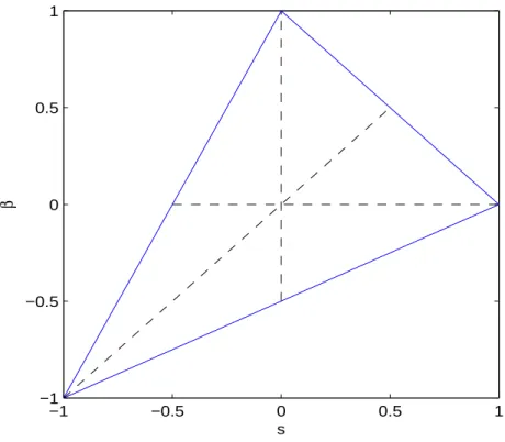
corresponding to the eigenvectorsni. The restrictions that 0≤di ≤1 and thatd1+d2+d3 = 1

place restrictions on the allowable values of sand β, as illustrated in Figure 1.3.

In calling n1 the major director, we have assumed that d1 is the unique largest eigenvalue

ofM. (This corresponds tos > β ands >0.) However, there are situations in which this is not

true. In a sense, ifd2 is the unique largest eigenvalue (This corresponds toβ > s,0.) then we

have simply chosen the wrong alignment for which to assignψ= 0, and there are no significant

physical differences between these cases. However, if d3 is the unique largest eigenvalue (or

s, β < 0), then the major director is n3 = (0,0,1), which corresponds to a logrolling state.

This means that the molecules are on average aligned orthogonal to thex-y plane rather than

parallel to it.

Additionally, there are special states in which there are repeated eigenvalues. The state

d1 = d2 = d3 = 1₃, that is s= β = 0, corresponds to the isotropic state of the fluid because

the pdf f(m) ≡ 1

−1 −0.5 0 0.5 1 −1

−0.5 0 0.5 1

s

β

Figure 1.3: The allowable values of the order parameters lie inside a triangle ins-β space. The dashed lines represent the uniaxial states.

there are only two distinct eigenvalues ofQare calleduniaxial states, in contrast to thebiaxial

states in which there are three distinct eigenvalues. These are depicted by the dashed lines in

Figure 1.3. The logrolling uniaxial stated3 > d1=d2 (s=β <0) is not significantly different

than a biaxial logrolling state. However, whend1 =d2 > d3 (s=β >0), the major director is

not well-defined, a degenerate situation that we will call adefect. The main feature of a defect

alignment is not that the molecules are on averageparallel to a special vector, but instead the

best that can be said is that on average, they areorthogonalto a special vector, in this casen3.

In other words, there is not one “favored” direction, but instead the molecules only agree to

reject one direction without reaching a consensus favorite. The two other uniaxial states with

defects are s= 0 withβ <0 and β = 0 withs <0, and they are aligned orthogonal to n₂ and

n1, respectively.

In terms of the probability density function f, in a biaxial state f(m) is an ellipsoid, but

at a uniaxial state,f is a spheroid. The defect states correspond tof being a oblate spheroid.

The alignments of remaining non-defect uniaxial statess= 0 withβ >0 andβ = 0 withs >0,

in whichf is an prolate spheroid, are not significantly different from those biaxial states nearby

ins-β space.

The system fors, β, ψ, and vx that we will analyze in this dissertation is

∂s

∂t = a3∂v∂yxg0(s, β) sin 2ψ−6Dr

¡

U(s) +2N sβ₃ (1−s+β)¢

−DrNL2

6

µ

(s−β)g0(s, β)

³

∂ψ ∂y

´₂ +1

2g1(s, β)∂ 2_s

∂y2 +1₂g2(s, β)∂ 2_β

∂y2

¶

+DrN L2

48

h

g3(s, β, ψ)∂ 2_ψ

∂y2 + (g4(s, β) +g5(s, β) cos 2ψ)∂ 2_s

∂y2

+(g6(s, β) +g7(s, β) cos 2ψ)∂ 2_β

∂y2 + (g8(s, β) +g9(s, β) cos 2ψ)

¡_∂ψ

∂y

¢₂

+2

3(−1 + 3 cos 2ψ)g1(s, β)

³

∂s ∂y

´₂

−2

3(1 + 3 cos 2ψ)g2(s, β)

³

∂β ∂y

´₂

+ sin 2ψ¡g10(s, β)_∂y∂s +g11(s, β)∂β_∂y

¢_∂ψ

∂y

+2 3

¡

−(1 + 3 cos 2ψ)g₁(s, β) + (−1 + 3 cos 2ψ)g₂(s, β)¢∂s ∂y∂β∂y

i ,

(1.34)

∂β

∂t =−a3∂v∂yxg0(β, s) sin 2ψ−6Dr

¡

U(β) +2N sβ₃ (1−β+s)¢

−DrNL2

6

µ

(s−β)g0(β, s)

³

∂ψ ∂y

´₂ +1

2g1(β, s)∂ 2_β

∂y2 +1₂g2(β, s)∂ 2_s

∂y2

¶

+DrN L2

48

h

−g3(β, s, ψ)∂ 2_ψ

∂y2 + (g4(β, s)−g5(β, s) cos 2ψ)∂ 2_β

∂y2

+(g6(β, s)−g7(β, s) cos 2ψ)∂ 2_s

∂y2 + (g8(β, s)−g9(β, s) cos 2ψ)

¡_∂ψ

∂y

¢₂

−2

3(1 + 3 cos 2ψ)g1(β, s)

³

∂β ∂y

´₂

−2

3(1−3 cos 2ψ)g2(β, s)

³

∂s ∂y

´₂

+ sin 2ψ¡−g10(β, s)∂β_∂y −g11(β, s)_∂y∂s

¢_∂ψ

∂y

+2 3

¡

(−1 + 3 cos 2ψ)g₁(β, s)−(1 + 3 cos 2ψ)g₂(β, s)¢∂s ∂y∂β∂y

i ,

(1.35)

∂ψ

∂t =−12∂v∂yx

³

1−a₃s+_s−β+2_β cos 2ψ ´

+DrNL2

24 s(s+−ββ+2)2_∂y∂

³

(s−β)2∂ψ ∂y

´

+DrN L2

16 (2 +s+β)

h

1 9(s−β)2_∂y∂

³

(2 +s+β)(s−β)2∂ψ ∂y

´

+ sin 2ψ ³

1+5s−4β

54(s−β) ∂ 2_s

∂y2 + 1+5_54(sβ₋−_β4₎s∂ 2_β

∂y2 + s−₃β

¡_∂ψ

∂y

¢₂´

−cos 2ψ³¡∂s_∂y+ ∂β_∂y¢∂ψ_∂y + s−₃β∂_∂y2ψ2

´i ,

(1.36)

∂vx

∂t = 1ρ

¡

− ∂p_∂x+∂τxy

∂y

¢

for the shear stress

τxy =

h

ηs+ 3νkBT

¡_ζ

1

6(s+β+ 2) + ζ42(s−β)2sin22ψ+ζ23

¢i_∂v

x

∂y

+3aνkBT

2 sin 2ψ

h

U(s)−U(β)−4N sβ₃ (s−β) i

+νkBT NL2

16

h¡ 1− a

3s+s−β+2β cos 2ψ

¢_∂

∂y

¡

(s−β)2∂ψ ∂y

¢

+a₃sin 2ψ ³

h0(β, s)∂ 2_β

∂y2 −h0(s, β)∂ 2_s

∂y2 + 2(s−β)(g0(s, β) +g0(β, s))

¡_∂ψ

∂y

¢₂´i

+νkBT N L2

32

h

h1(s, β, ψ)∂ 2_ψ

∂y2 +h2(s, β, ψ)∂ 2_s

∂y2 −h2(β, s, ψ)∂ 2_β

∂y2 +h3(s, β, ψ)

¡_∂ψ

∂y

¢₂

+a₉sin 2ψ ³

(−1 + 3 cos 2ψ)h0(s, β)

³

∂s ∂y

´₂

+ (1 + 3 cos 2ψ)h0(β, s)

³

∂β ∂y

´₂´

+(h3(s, β) +h4(s, β) cos 2ψ)∂s_∂y+ (h3(β, s)−h4(β, s) cos 2ψ)∂β_∂y

¢_∂ψ

∂y

+h₅(s, β, ψ)∂s ∂y∂β∂y

i

(1.38)

where

U(s) =s¡1−N₃(1−s)(2s+ 1)¢, g0(s, β) = 1 + 2s−β+ 3sβ−3s2,

g₁(s, β) = (s−1)(1 + 2s−β), g₂(s, β) =s(1−s+ 2β),

g3(s, β, ψ) = 2 sin 2ψ(1 +s)(s−β)(1 +s+β−2(s2−sβ+β2)),

g₄(s, β) =−1

3(1 +s)(8s2+sβ−4s−4−β2+ 5β)

g5(s, β) = 1₉(2(s−1)(1 + 2s)(5 + 18s) + 17β+ 22sβ−99s2β+ 45sβ2−7β2),

g₆(s, β) = 1

3s(s2+ 4s−17β−sβ−8β2−5)

g7(s, β) = 1₉(17s+ 20s2−9s3+ 99s2β−5sβ−16β2−72sβ2+ 8β+ 8),

g₈(s, β) =−2

3(s−β)

¡

4 + 13s−8s2_−9s3_{−5β+ 11sβ+β}2_{+ 9sβ}2¢_,

g9(s, β) =−2(s−β)(−2 + 13s3+β+β2−4s2−22s2β−7s+ 3sβ+ 13sβ2)

¢ ,

g10(s, β) =−4(−1 + 4s3−5s2β+β2+s(−3 +β(3β−1))),

g11(s, β) =−4(1 + 2s−3s3+β+ 2sβ+ 5s2β−2β2−4sβ2),

(1.39)

h₀(s, β) = (1−β+ 2s)(1 +β−s),

h1(s, β, ψ) = 1₃(s−β)2(2 +s+β−3(s−β) cos 2ψ)−₁₈a(s−β)2

³

2 cos 2ψ(2+_ss₋+_ββ)2

−3¡1 + 2(s2_−sβ+β2_{) + cos 4ψ(3−2s}2_{+ 2β−2β}2_{+ 2s+ 2sβ)}¢´_,

h2(s, β, ψ) = ₁₈1 sin 2ψ

h

a(8s3+ 4s2−7s2β+ 3β2+β2−8s−11sβ−2sβ2−4

−3 cos 2ψ(s−β)(8s2_{+ 5β}2_{−β−3s−11sβ−3)) + (1 + 5s−4β)(s−β)}i_,

h₃(s, β, ψ) = sin 2ψ(s−β) ³

(s−β)2₋a

9

¡

9s3_{+ 7s}2_−9s2_{β−8s−9sβ}2_−13sβ+

+9β3_−7β2_{−8β−8 + 3(s−β) cos 2ψ(10−13s}2_{+ 6s+ 22sβ+ 6β−13β}2₎¢´_,

h4(s, β) =−3(s−β)2−a₉(2 +s+β)(4 + 3s+β),

h5(s, β, ψ) = a₉sin 2ψ

³

(s−β)(s+β−1)

+3 cos 2ψ(3s2_{+ (β−1)(2 + 3β)−s(1 + 6β))}´_.

(1.40)

1.8

Rheological Properties

One motivation for solving the system (1.34)-(1.38) is that once the stress tensor is known, we

are able to make predictions of certain rheological properties that can be measured in laboratory

experiments (Larson, 1999).

1.8.1 Storage and Loss Moduli

In a perfectly neo-Hookean solid, the shear stress is proportional to the shear strainγ:

τ_xyneo−Hookean=Gγ, (1.41)

for the shear modulusG. For a perfectly Newtonian fluid, however, the shear stress is

propor-tional to the strain rate ˙γ:

τ_xyN ewtonian=ηγ,˙ (1.42)

for the shear viscosityη. It is assumed that the strain and strain rate are macroscopic quantities

defined for the system as a whole, and not defined locally inside the substance so that the stress

response is also homogeneous, and the shear modulus and viscosity are material properties.

similar to both a neo-Hookean solid and a Newtonian fluid. One method to probe the

com-bination of these two dissimilar elements is through linear viscoelasticity. In this case, it is

expected that the velocity gradient is approximately linear iny and oscillatory in time so that

the macroscopic shear strain can be written as

γ =γ₀sinωt. (1.43)

The macroscopic strain rate is then just

˙

γ = ˙γ0cosωt, (1.44)

where ˙γ0 =γ0ω. Thus, a measure of a substance’s solid-like and liquid-like properties can be

made if the shear stressτ_xy can be decomposed into the sum of a part in-phase with the strain

and another out-of-phase (or in-phase with the strain rate):

τxy =γ0

¡

G0(ω) sinωt+G00(ω) cosωt¢. (1.45)

The in-phase termG0(ω) is called thestorage modulusand the out-of-phase termG00(ω) is called

theloss modulus. To mimic the notation in (1.43), thecomplex modulus is

G∗=G0+iG00. (1.46)

Alternatively, from the perspective of (1.44), thecomplex viscosity is defined as

η∗ =η0−iη00= G

∗

iω. (1.47)

The ratio

G00

G0 = tanδ (1.48)

is known as the loss tangent, and it is large for a substance that is more liquid-like and small

for a substance is more solid-like.

The ultimate goals of the chapters that follow are to make predictions of the storage and

lose moduli.

1.8.2 Normal Stress Differences

Two other important rheological properties are the first and second normal stress differences,

defined by

N1 =τxx−τyy,

N2 =τyy−τzz,

(1.49)

respectively. Non-zero normal stress differences indicate a force exerted by the fluid pushing

Chapter 2

Shear flow in the monodomain Limit

In the so-called “monodomain limit,” it is assumed that there are no spatial gradients in the

ori-entation variables, which in turn allows us to remove hydrodynamic feedback from the problem.

Therefore, it allows us to impose a linear velocity profile and then compute the orientation’s

reaction. A modified version of this chapter appears in Choate and Forest (2006).

2.1

Monodomain limit and nondimensionalization

In the monodomain limit, the interaction lengths L and L are assumed to be small compared

to the length scale over which distortions occur, allowing us to effectively ignore the spatial

gradients in the system (1.34)-(1.38). Thus, we can assume that for small amplitude oscillatory

shear flow the velocity is simply linear iny, and we will write it as

vx = ˙γ0ycosωt, (2.1)

where ˙γ0= A_h0ω is a shear rate composed of the gap width h, the maximum relative amplitude

of the oscillatory displacement of the parallel platesA₀, and the frequency of the oscillation ω.

This crude simplification is indeed shown to be physically relevant for the fluid near the center

of the channel when the plate separation is wide.

Under these restriction thats,β, andψ are functions of time only, the system (1.34)-(1.36)

reduces to

˙

s= −6Dr

¡

U(s) + 2N sβ₃ (1−s+β)¢+ a₃γ˙0cosωt(1 + 2s−β+ 3sβ−3s2) sin 2ψ,

˙

β = −6Dr

¡

U(β) +2N sβ₃ (1−β+s)¢−a₃γ˙0cosωt(1 + 2β−s+ 3sβ−3β2) sin 2ψ,

˙

ψ= −1₂γ˙0cosωt

³

1−a₃s+_s−β+2_β cos 2ψ ´

,

and it is this system of ordinary differential equations that we we analyze in this chapter.

As a characteristic timescale we choosetr = (6Dr)−1, the timescale of molecular rotational

diffusion. For small molecule liquid crystals, this timescale is quite fast; however, from (1.18),

for the larger polymeric molecules of the present discussion, the rotational diffusion is slow

enough to have an observable effect. In this dissertation, we will use Dr = 35 s−1. Thus, the

nondimensional velocity is

v_x =De ycosωt (2.3)

where we have defined the nondimensionalDeborah number

De= γ˙0

6Dr (2.4)

as the ratio of the shear rate to the rate of rotational diffusion so that the small amplitude limit

isDe <<1. The system (2.2) reduces to

˙

s=−U(s)−2N sβ₃ (1−s+β) +a₃Decosωt(1 + 2s−β+ 3sβ−3s2) sin 2ψ, (2.5)

˙

β=−U(β)−2N sβ₃ (1−β+s)−a₃Decosωt(1 + 2β−s+ 3sβ−3β2) sin 2ψ, (2.6)

˙

ψ=−1₂Decosωt ³

1−a₃s+_s−β+2_β cos 2ψ ´

. (2.7)

2.2

Degenerate quiescent equilibrium

The system (2.5)-(2.7) possesses very special equilibrium solutions when there is no flow, that

is, when De= 0. In this case we find that (2.5)-(2.7) reduces to

˙

s = −U(s)−2N sβ

3 (1−s+β) (2.8)

˙

β = −U(β)−2N sβ

3 (1−β+s) (2.9)

˙

or in its equivalent tensor form

˙

Q=Q−N(M·M−M:MM). (2.11)

From (1.39),U(s) =s(1−N₃(1−s)(2s+ 1)), and so the only material parameter in this system

is the nondimensional concentration parameter N.

In general, the equilibrium order parameter system (2.8)-(2.9) has seven steady solutions,

but for the purposes of this dissertation, we will ignore the five solutions that are unstable to

perturbations in the form of a shear flow for all N >0 (Forest and Wang, 2003)). One of the

remaining two solutions is the isotropic solution

(s, β) = (0,0), (2.12)

which exists for allN > 0 but is only stable for 0< N <3. This solution corresponds to the

state in which the molecules have no preferred orientation either because the concentration is

too low for the molecules to effective communicate with each other or because the temperature

is too high.

Additionally, if the concentration is sufficiently high,N > 8₃, then there is also the uniaxial

nematic equilibrium solution

(s, β) = (s_eq,0) (2.13)

for

seq = 1₄

à 1 + 3

r 1− 8

3N !

. (2.14)

This solution is stable if it is defined. Thus, in the region 8

3 < N < 3, the isotropic and

nematic solutions are bistable, but when N > 3, (seq,0) is the only solution stable to shear

perturbations. For the remainder of this dissertation, we will assume that N is well into the

nematic range, using N = 6 so that seq = 0.809.

While the concentration selects the degree to which the molecules are ordered, in the absence

of flow, the preferred direction of this ordering is not selected. Indeed, from (2.10), any constant

value

ψ≡Ψ₀ (2.15)

is a solution. (We choose −π₂ < Ψ0 ≤ π₂.) Several authors (cf. (Forest et al., 2003; Hess and

Kr¨oger, 2004; Leeet al., 2006; Marrucci and Greco, 1993; Rien¨acker and Hess, 1999; Rien¨acker

et al., 2002a,b)) have explored the role of this orientational degeneracy in steady shear.

In the following, we will use this orientationally degenerate equilibrium solution as our initial

conditions for (2.5)-(2.7):

s(t= 0) =seq, β(t= 0) = 0, ψ(t= 0) = Ψ0. (2.16)

We shall see that some phenomena are sensitive to the initial value of the director angle.

2.3

Weak steady shear flow

Before we examine weak oscillatory shear, we will first look at weak steady shear, or De <<1

withω= 0 in (2.5)-(2.7).1 _{We will employ “two-timing” asymptotic analysis similar to that used}

in (Vicente Alonso et al., 2003) for a Landau-de Gennes model. The utility of this asymptotic

analysis is that one can effectively diagonalize the fast and slow response of the director and

order parameters, and thereby solve the system (2.5)-(2.7) in a hierarchy of simpler, lower

dimensional equations. The molecular relaxation timescale

T0 =t (2.17)

dominates the order parameter equations (2.5)-(2.6) while the director angle equation (2.7) is

on the slower shear flow timescale

T1 =De t. (2.18)

1_{As defined by (2.4), whenω= 0, thenDe= 0, and indeed,v}

x in (2.1) is 0. Therefore in steady shear, we

will define the Deborah number asDe= γ˙0

We treat the initial slow time as zero, but we allow for the initial value of the fast timeT00=t0

to be a free parameter, the role of which will be discussed below. We will use the expansions

s = s_eq+De sss₁ (T₀, T₁) +O(De2), (2.19)

β = 0 +De βss₁ (T₀, T₁) +O(De2), (2.20)

ψ = ψ₀ss(T₀, T₁) +De ψ₁ss(T₀, T₁) +O(De2), (2.21)

where the superscript ss denotes steady shear. Alternatively, the orientation tensor can be

expanded as

Q= s_eq¡nss

1,0nss1,0−I3

¢

+De h

sss

1

¡ nss

1,0nss1,0− I3

¢ +βss

1

¡ nss

2,0nss2,0−I3

¢

+seqψss1

¡ nss

1,0nss2,0+nss2,0nss1,0

¢i

+O(De2_),

(2.22)

wherenss

1,0= (cosψ0ss,sinψ0ss,0) and n2ss,0= (−sinψss0 ,cosψ0ss,0).

At zeroth order in De, we quickly see that ∂ψ0ss

∂T0 = 0, and so at first order (2.7) yields

∂ψss

1

∂T0 =−

dψss

0

dT1 − 1

2(1−λ0cos 2ψss0 (T1)), (2.23)

where we have define the Leslie tumbling parameterλ₀=λ(s_eq,0) with

λ(s, β) = a 3

2 +s+β

s−β . (2.24)

Integrating (2.23) with respect toT0, we see that

ψss

1 (T0, T1) =−T0

³

dψss

0

dT1 + 1

2(1−λ0cos 2ψ0ss(T1))

´ + ¯ψss

1 (T1), (2.25)

The solvability condition that ψ₁ss remains bounded as a function ofT0 yields

dψss

0

dT1 =− 1

2(1−λ0cos 2ψss0 ). (2.26)

Thus one recovers the well-known director angle equation from Leslie-Ericksen theory, which

comes from (1.4) in the in-plane monodomain limit. It is separable and can be integrated in

closed form, which we represent by ψ₀ss(T1) = Ψ(T1+φ0), where

Ψ(x) =               

tan−1

µ_√

1−λ2 0 1+λ0 tan

µ

− √

1−λ2 0 2 x

¶¶

, if|λ₀|<1,

tan−1

µ

tanψLtanh

µ√

λ2 0−1 2 x

¶¶

, if|λ0|>1 and|Ψ0|<|ψL|,

tan−1

µ

tanψLcoth

µ√

λ2 0−1 2 x

¶¶

, if|λ0|>1 and|ψL|<|Ψ0|< π₂,

(2.27)

where

ψL= tan−1

à p λ2

0−1

λ0+ 1

!

(2.28)

is the classical Leslie angle, and

φ0 =

            

−√2

1−λ2 0

tan−1

µ

1+λ0

√

1−λ2 0

tan Ψ0

¶

, if|λ0|<1,

2

√

λ2 0−1

tanh−1 ³

tan Ψ0 tanψL

´

, if|λ₀|>1 and |Ψ₀|<|ψ_L|,

2

√

λ2 0−1

coth−1 ³

tan Ψ0 tanψL

´

, if|λ0|>1 and |ψL|<|Ψ0|< π₂.

(2.29)

Thus if |λ0| < 1, then ψ0ss(De t) is periodic with period Tss = _De√2π_1−λ2 0

, meaning that

the director tumbles. However, if |λ₀|> 1, then the director aligns relative to the flow with

ψss

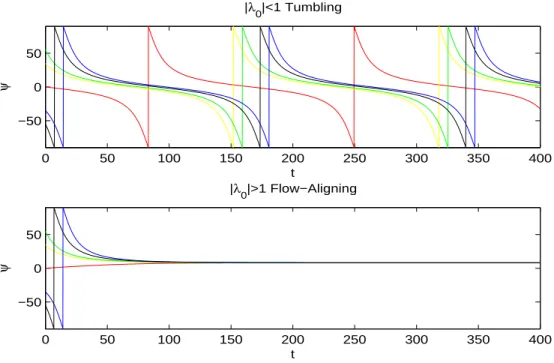
0 (De t) decaying to the Leslie alignment angleψL. These two different behaviors are depicted

for rods in Figure 2.1 and for disks in Figure 2.2.

To our knowledge the exact role of the initial director angle Ψ0 has not been previously

amplified. It is often hidden in a generic constant of integration and sometimes taken to be zero.

This is understandable since the qualitative effect of Ψ0 on ψ0ss is not significant, introducing

only a phase shift in the tumbling regime, and in the flow-aligning case only affecting the

direction from which the director approaches the Leslie angle (ψss

0 will not pass through −ψL

on its way toψL), as illustrated in Figure 2.1. We shall show below, however, that the effect of

0 50 100 150 200 250 300 350 400 −50

0 50

t

ψ

|λ

0|<1 Tumbling

0 50 100 150 200 250 300 350 400

−50 0 50

t

ψ

|λ₀|>1 Flow−Aligning

Figure 2.1: The two different responses, tumbling and flow-aligning, to steady shear for rods with a = 0.8 (λ0 = 0.926) and 0.9 (λ0 = 1.042) for Ψ0 = −55◦,−35◦,0◦,35◦, and 55◦. For

a= 0.9,ψL= 8.128◦. [N = 6, De= 0.1.]

0 50 100 150 200 250 300 350 400

−50 0 50

t

ψ

|λ

0|<1 Tumbling

0 50 100 150 200 250 300 350 400

−50 0 50

t

ψ

|λ₀|>1 Flow−Aligning

Figure 2.2: The two steady shear responses for disks with a=−0.8 (λ0 =−0.926) and −0.9

(λ0 =−1.042) for Ψ0 =−55◦,−35◦,35◦,55◦,and ±90◦. For a=−0.9,ψL=−81.87◦. [N = 6,

De= 0.1.]

Usingψss

0 (T1), the O(De) order parameter equations are triangular system

∂βss

1

∂T0 = −a1β

ss

1 +aa4sin 2ψ0ss(T1),

∂sss

1

∂T0 = −a2s

ss

1 +a3β1ss+aa5sin 2ψ0ss(T1),

(2.30)

where

a1 = N₃

¡ 2s2

eq+ 2seq−1 +_N3

¢

=N seq

a₂ = N

3

¡ 6s2

eq−2seq−1 +_N3

¢ = N

3

¡

s_eq+ 2− 6

N

¢ ,

a3 = 2₃N

¡ s2

eq−seq

¢

= 1₂(a2−a1),

a4 = 1₃(seq−1),

a5 = 1₃

¡

1 + 2seq−3s2eq

¢

= 1₆(seq−1 +_N9).

(2.31)

This can be solved exactly by quadrature:

β₁ss(T0, T1) = asin 2ψ0ss(T1)a_a4₁

¡

1−ea1(T00−T0)¢_,

sss

1 (T0, T1) = asin 2ψ0ss(T1)

³

a3a4+a5a1

a1a2 −

a4 2a1e

a1(T00−T0)₊a4−2a5 2a2 e

a2(T00−T0)

´ ,

(2.32)

The two order parameter relaxation rates a1 and a2 are the same rates identified in (Larson

and Mead, 1989a). In the nematic regionN >3,a₁ > a₂> 1

2. However, in the bistable region 8

3 < N < 3,a2 →0 as N → 83.

Thus for steady shear, at leading order the tensor model predicts the same director

behav-ior as Leslie-Ericksen theory coupled with order parameters that decay exponentially to the

quiescent uniaxial values modified byO(De) corrections that are proportional to sin 2ψss

0 . The

main parameter in determining qualitative behavior is the Leslie “material parameter”λ0 which

is identified for nematic polymers as dependent on aspect ratio through a and concentration

through seq (Forest and Wang, 2003).

Using (2.32), the analysis can be continued to get ¯ψss₁ . AtO(De2), (2.7) is

∂ψss

2

∂T0 =−

dψ¯ss

1

dT1 −

a2 3s2

eq

³

(seq(seq+ 2) ¯ψss1 sin 2ψ0ss+

a

2sin 4ψ0ss

³

a3a4+a1a5−a2a4(1+seq)

a1a2 +

a4(2seq−1)

2a1 e

a1(T00−T0)₊a4−2a5 2a2 e

a2(T00−T0)

´ ´ .

(2.33)

We observe that for ψss

2 to be bounded as a function of T0, we must require that d ¯

ψss

1

the flow-aligning regime, it is easy to solve (2.33) for this constant ¯ψss

1 in the limit T0 → ∞.

This can improve the approximation to the flow-alignment angle to

ψ_L+De3((seq+ 1)a4a2−a3a4−a1a5) a1a2(seq+ 2)2

. (2.34)

Also, the first order asymptotic expressions for the order parameters are

s =seq+Dea(a3a_a4₁+_a2a5a1)sin 2ψL,

β =Deaa4

a1 sin 2ψL.

(2.35)

2.4

Weak Oscillatory Shear Flow

2.4.1 Leslie-Ericksen for weak oscillatory shear flow

Anticipating a similar relationship between the tensor and Leslie-Ericksen models for the more

complicated dynamics of oscillatory shear, we begin our investigation of oscillatory shear with

the non-autonomous generalization of the LE director angle equation,

dψ_LE

dt =−

1

2Decosωt(1−λ0cos 2ψLE). (2.36)

This equation can also be solved exactly:

ψLE(t) = Ψ

µ

Desinωt−sinωt0

ω +φ0

¶

, (2.37)

where the function Ψ is defined by (2.27). This solution predicts an oscillatory response for

both “tumbling” and “flow-aligning” nematic liquids as classified based on their steady shear

response. This oscillatory behavior is a consequence of the “internal clock,” De_ω sinωt, which

oscillates between ±De_ω , on which the with function Ψ is evaluated. Thus the director angle

oscillates about the initial angle Ψ0.

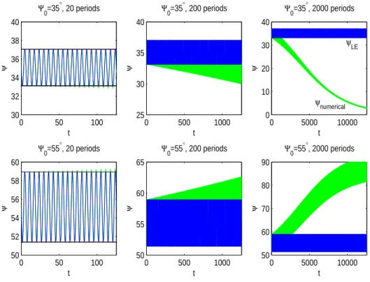
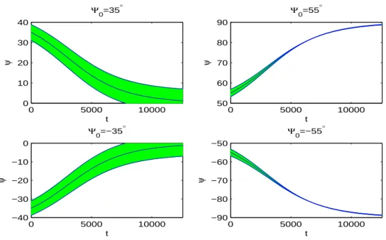
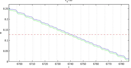
Figure 2.3 comparesψLE to a numerical solution of the tensor model (2.5)-(2.7) whereψ,s,

and β are coupled. We observe: ψLE accurately captures the oscillatory nature of the director

anglefor small times, a few dozen periods of the plates. However, for larger times, a slow drift

of the mean director angle of the tensor model emerges, and furthermore the drift dynamics

0 50 100 50

52 54 56 58 60

t

ψ

Ψ₀=55°, 20 periods

0 500 1000

50 55 60 65

t

ψ

Ψ₀=55°, 200 periods

0 5000 10000

50 60 70 80 90

t

ψ

Ψ₀=55°, 2000 periods

0 50 100

30 32 34 36 38 40

t

ψ

Ψ₀=35°, 20 periods

0 500 1000

25 30 35 40

t

ψ

Ψ₀=35°, 200 periods

0 5000 10000

0 10 20 30 40

t

ψ

Ψ₀=35°, 2000 periods

ψ_LE

ψ_numerical

Figure 2.3: The Leslie-Ericksen theory prediction (dark band) of oscillation around the initial value Ψ₀ coincides with the numerical solution (light band) for the first few plate oscillations, but the mean of the numerical solution slowly drifts toward either 0◦ _{(if |Ψ}

0|<45◦) or ±90◦

(if 45◦ _{< |Ψ}

0| <90◦). [N = 6, a = 0.8 (λ0 = 0.926), De = 0.1, andω = 1 for Ψ0 = 35◦ and

Ψ₀= 55◦_.]

are sensitive to initial data.

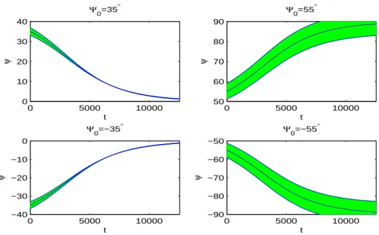
More complete numerical studies show the asymptotic value of the mean angle is parallel

to the plates when |Ψ0|< π₄ or perpendicular to the plates when π₄ <|Ψ0|< π₂. For the LE

model, the asymptotic value of the mean is simply Ψ₀, independent of the initial data, and

independent of the Leslie parameter λ0.

2.4.2 Failure of the two-timing argument used for steady shear

Before using multiple timescale perturbation analysis in oscillatory shear, we must briefly discuss

the additional timescale introduced when ω 6= 0. We limit the present discussion to relatively

fast plate oscillation, or ω >> De, and use cosωt = cosωT₀ when time appears explicitly

in (2.5)-(2.7). Additionally we note that we have used the term “mean” loosely, for indeed

ω

2π

R_t+π ω

t−_ωπ ψLE(t0)dt0 6= Ψ0 (unless Ψ0 = 0), but instead

R_t+π ω

remainder of the paper we use “mean” to refer to integrating with respect toT0 only over one

period allowing the mean to remain a function of the slow timeT1.

If the two-timing argument from Section 2.3 is followed again for oscillatory shear, we still

have ∂ψ0

∂T0 = 0 so thatψ0(T0, T1)≡

˜

ψ0(T1), but (2.25) becomes

∂ψ1

∂T0 =−

dψ˜0

dT1 −

1

2cosωT0 ³

1−λ0cos 2 ˜ψ0(T1)

´

. (2.38)

After integration with respect toT0, one finds that

ψ1(T0, T1) =−(T0−T00)d_dTψ˜₁0 −sinωT0−_2ωsinωT00

³

1−λ0cos 2 ˜ψ0

´

+ ˜ψ1(T1). (2.39)

Thus, the solvability condition for ψ₁ to remain bounded as a function of T₀ is now dψ˜0

dT1 = 0,

implying that ψ0(T0, T1) ≡ Ψ0, which clearly does not capture the long time dynamics of the

numerical solutions shown in Figure 2.3. We shall see that in fact this longtime drift of the

mean of the oscillation arises from the emergence of higher harmonics in the O(De2_{) balance,}

arising precisely through the small amplitude oscillations of the tumbling parameter λ(s, β).

Thus, LE theory with its constant order parameter cannot yield this effect.

2.4.3 A third slower timescale

Since the two times T₀ = t and T₁ = De t do not prove to be enough to capture the drift in

Figure 2.3, we will introduce a new, slower time T2 = De2t. Instead of ψ0(T0, T1) ≡ Ψ0 of

the previous section, we now allow ψ0(T0, T1, T2)≡ ψ¯0(T2), and replace ˜ψ1(T1) in (2.39) with

˜

ψ1(T1, T2).

Even though ¯ψ0(T2) is not yet known, it does not prevent us from solving the system for

the order parameters at O(De):

∂β1

∂T0 = −a1β1+aa4cosωT0sin 2 ¯ψ0(T2),

∂s1

∂T0 = −a2s1+a3β1+aa5cosωT0sin 2 ¯ψ0(T2),

(2.40)

where theai are given by (2.31). This system can be solved by quadrature, and we see that the

order parameters quickly decay to sinusoidal states with an amplitude that may vary slowly