Investigation of Pulse Shape
Discrimination Using a
Convolutional Autoencoder for the
Baksan Experiment on Sterile
Transitions
Thomas Marshall
Senior Honors Thesis
Department of Physics and Astronomy
University of North Carolina at Chapel Hill
March 31, 2020
Approved:
Dr. John Wilkerson, Thesis Advisor
Dr. Reyco Henning, Reader
Investigation of Pulse Shape Discrimination Using a
Convolutional Autoencoder for the Baksan Experiment on Sterile
Transitions
Thomas Marshall
11University of North Carolina - Chapel Hill, Chapel Hill, North Carolina 27514
March 31, 2020
Abstract
The Baksan Experiment on Sterile Transitions (BEST) is a short-baseline neutrino oscillation ex-periment that aims to explore an observed deficit in the measured neutrino flux of calibration sources from the radiochemical solar neutrino experiments, SAGE and GALLEX. To maximize sensitivity of the experiment, effective pulse shape discrimination (PSD) of experimental signals is crucial. The viability of a convolutional autoencoder used to achieve good PSD among BEST waveforms is explored through testing on a 2014 data set from the precursor to BEST, the Russian American Gal-lium Experiment (SAGE). Waveforms from this data set were condensed to 5 parameter descriptions through this neural network and used to discriminate background events from candidate71Ge decay events. For the 10.4 keVK peak of71Ge, there was 91.7% agreement (plus 13.5% additional event acceptance) between BESTnet’s list and events found in the official list. For the 1.2 keVLpeak of
71
Ge, there was 35.4% agreement (plus 28.0% additional event acceptance) between BESTnet’s list and events found in the official list. These results suggest reasonable performance of the network above 5 keV, but improvements are needed for performance at low energies below this threshold.
1
Physics Motivation
1.1
Neutrinos
Neutrinos, ν, are leptons within the Standard Model of Particle Physics. They are extremely light particles with an unknown absolute mass scale that interact solely via the weak interaction and are observed in the form of three known flavors: electron, muon, and tau. First proposed by Wolfgang Pauli in 1930 [1], neutrinos were not experimentally observed until the mid 1950s by the Cowan-Reines experiment [2]. Their confirmed detection opened the door for further experimental searches using the neutrino, such as direct measurements of solar and other astrophysical phenomena. Among several of these searches, deficits in the observed rate of the phenomenon compared to the theoretically predicted rate arose, leading to a plethora of explanations for the difference in results [3].
Neutrino flavor oscillation arose as the solution to these issues after a great deal of deliberation and further experimentation. The Homestake, Super-Kamiokande, and Sudbury Neutrino Observatory Ex-periments each played a major role in proposing and confirming the existence of flavor oscillation in neutrinos, with Nobel Prizes being awarded to the leaders of each of these collaborative efforts [3][4][5]. This phenomenon arises uniquely in neutrinos through quantum superposition of states. For most par-ticles, their flavor eigenstate aligns perfectly with their energy and mass eigenstates. For neutrinos, however, this is not the case. Instead, the Pontecorvo-Maki-Nakagawa-Sakata (PMNS) mixing matrix shown below provides a description of the mapping of the neutrino mass eigenbasis onto its flavor eigen-basis for the three known flavors of neutrinos.
|νei
|νµi
|ντi
=
Ue1 Ue2 Ue3
Uµ1 Uµ2 Uµ3
Uτ1 Uτ2 Uτ3
|ν1i |ν2i |ν3i
(1)
the mapping of one mass eigenstate,y, onto a flavor eigenstate,x. This matrix is theoretically expressed as the product of four matricies in terms of six parameters: θ12, θ13, θ13, δCP, α1, and α2. Each θ
parameter describes the neutrino mixing angle between flavors, α1 and α2 are Majorana phases which
are only non-zero if neutrinos are their own antiparticles, andδCP signifies the magnitude of CP violation apparent in neutrino oscillation. Lettingcij ≡cos (θij) andsij ≡sin (θij) the following matrix is created:
U =
1 0 0 0 c23 s23
0 −s23 c23
c13 0 s13e−iδCP
0 1 0
−s13eiδCP 0 c13
c12 s12 0 −s12 c12 0
0 0 1
eiα1/2 0 0
0 eiα2/2 0
0 0 1
(2)
The best measured values of these parameters as of 2018 from the Particle Data Group are provided as a reference for a sense of scale as well [6]. Completing this inner product between matricies using
sin2(θ12) sin2(θ23) sin2(θ13) δCP Normal Mass Ordering (Octant I) 0.307±0.013 0.512±0.022 (2.18±0.07)×10−2 1.37±0.18
Normal Mass Ordering (Octant II) 0.307±0.013 0.542±0.022 (2.18±0.07)×10−2 1.37±0.18
Inverted Mass Ordering 0.307±0.013 0.536±0.028 (2.18±0.07)×10−2 1.37±0.18
Table 1: Particle Data Group 2018 reported parameter values for 3-flavor neutrino oscillation.
α1andα2values not provided because the Majorana nature of neutrinos has not been definitively
determined yet. [6]
measured mixing values, each respectiveUαi element of the matrix in equation 1 is produced.
Neutrinos are only detected through the weak interaction via their respective flavor eigenstates. Thus, neutrinos will always be created and observed in a flavor eigenstate. Starting with a flavor eigenstateα
and using the PMNS mixing matrix, the initial state of the particle as a superposition of mass eigenstates is given by:
|να(t)i=
X
k
Uαke−iEkt|νki (3)
where Roman letters will represent mass eigenstates and Greek letters will represent flavor eigenstates. Neutrinos cannot be detected in mass eigenstates, so the mass eigenstate superposition is converted into a flavor eigenstate superposition through the PMNS matrix again to get:
|να(t)i=X β
X
k
UαkUβk∗ e
−iEkt|ν
βi (4)
This yields a complete description of the time evolution of a neutrino produced in an initial flavor eigenstate, α. To determine the probability that this neutrino is observed in another flavor eigenstate,
β, at a later time,t, the overlap between the two eigenstates,Aα→β=hνβ|να(t)i, must be determined. From this, the squared amplitude ofAα→β determines the probability of oscillation yielding:
Pα→β=|Aα→β|2=
X
k,j
UαkUβk∗ Uαj∗ Uβje−i(Ek−Ej)t (5)
Assuming neutrinos travel at speeds very near the speed of light and using Lorentz-Heaviside natural units, the approximationsEk 'E+
m2
k
2E and t 'L are made, wheremk is the mass of neutrino mass eigenstatek andL is the length traveled by the neutrino following its creation in the flavor eigenstate,
α. Combining these approximations and using Euler’s identities, an equation for the probability that a neutrino produced in flavor eigenstate, α, oscillates into another eigenstate, β, over some distance, L, with energy,E is produced:
Pνα→νβ =δαβ−4
X
k>j
Re[UαkUβk∗ U
∗
αjUβj] sin
2 ∆m 2 kjL 4E ! +2X k>j
Im[UαkUβk∗ Uαj∗ Uβj] sin ∆m2
kjL 2E
! (6)
in sign for the third term in the equation [7, Chapter 5]. The ∆m2kj andUxy values mentioned in this derivation are experimentally measured, rather than theoretically predicted.
The confirmed observation of this phenomenon requires that in order for these oscillations to occur, the sine terms must be nonzero. This, in turn, requires the mass squared differences between neutrino mass eigenstates to also be nonzero. Thus, at least two of the three neutrino mass eigenstates must be nonzero for neutrino oscillations to occur. Experimental observation ofν oscillations provides the first direct, irrefutable contradiction to the Standard Model.
1.1.1 Sterile Neutrinos
These observations led to further experimental attempts aimed at improving the accuracy and pre-cision of the parameters which characterize the nature of the oscillation. One such attempt aimed at searching for antineutrino oscillations was the Liquid Scintillator Neutrino Detector (LSND) experiment. This experiment sought to create the decay products νe,νµ, andνµ, but not νe, using a beam of pro-tons that produced predominantly positively-charged pions when incident on a target. Through inverse beta decay, the experiment searched for evidence of νe events that would have occurred through flavor oscillations via theνµs. A nearly 4σexcess ofνeevents was observed, but with a large ∆m2in the range of 0.2-10 eV2/c4 [8]. At a mass squared difference this large, the results observed by the experiment
strongly contradicted the values widely accepted under the 3-active-flavor oscillation theory resulting in an anomaly that has yet to be completely resolved [9].
Similar neutrino oscillation excesses and deficits were observed in a variety of other experiments as well. In the Mini Booster Neutrino Experiment (MiniBooNE), an attempt to test the LSND anomaly, an even larger excess of events cited at 4.7σ was observed for similar L/E conditions leading to a likely ∆m2 of the same magnitude as the LSND results [10]. Among reactor neutrino experiments exploring oscillation parameters in the three flavor framework such as CHOOZ, KamLAND, and Daya Bay, a 2.8σcombined deficit in expected neutrino flux between all experiments was observed leading to a claimed reactor antineutrino anomaly (RAA) [9][11]. The sudden rise in observed experimental anomalies surrounding neutrino oscillations left many questions about the possible sources of the anomalies and whether or not they might be related. To provide a possible explanation, additional neutrino flavors (typically between 1-3) which only interact via neutrino mixing and not the weak interaction were proposed.
Additional sterile neutrino flavors have been proposed through a variety of different mechanisms [12]. The (3+1) flavor mixing scheme is explored for the purposes of this paper. Through this scheme, one additional neutrino flavor is added to the current model with right-handed chirality so as to keep it from interacting via the weak interaction. Adding this additional flavor to the current three flavor framework creates a modified PMNS matrix:
|νei
|νµi
|ντi
|νsi
=
Ue1 Ue2 Ue3 Ue4
Uµ1 Uµ2 Uµ3 Uµ4
Uτ1 Uτ2 Uτ3 Uτ4
Us1 Us2 Us3 Us4
|ν1i |ν2i |ν3i |ν4i
(7)
where thesflavor eigenstate and fourth mass eigenstate represent those of the additional sterile neutrino. This assumes that the current 3-flavor PMNS matrix would be slightly non-unitary, requiring the addition of a fourth flavor to preserve unitarity. What makes this proposed mechanism so appealing is the ease with which it would incorporate itself with the current three-flavor oscillation model. Using the new PMNS matrix with four-by-four dimensions instead of three-by-three, the same oscillation probability description given through equation (6) would apply with only the addition of an extra item to compute in each sum and slightly differentUαi values.
flavors. Under resonant experimental oscillation conditions for the additional flavor (4E∼∆m2sL) and assuming a 3-flavor model, flavor oscillation would be unexpected because the sine terms in equation (6) would be small for such tiny mass splittings. Under the (3+1) model, however, flavor oscillation would be possible through coupling of the active flavors to the additional sterile flavor. This phenomenon would allowνµ ↔ νe oscillation like that observed in the LSND and MiniBooNE experiments that would be otherwise not possible [9].
It is important to note that although this model provides a relatively painless solution to neutrino oscillation anomalies, it is not the only proposed solution and has flaws. Some studies favor a (3+2) model over the simpler (3+1) model, making the (3+1) solution less attractive compared to alternative proposed options [13]. For specific anomalies, other non-sterile-neutrino-based explanations are also often deemed viable. For the LSND anomaly, some studies have questioned the magnitude and significance of the anomalous results, lowering the excess from nearly 4σ to less than 3σ [14]. For the RAA, poor knowledge of the expected antineutrino flux produced by specific reactor fuel can also be attributed as a possible cause of the observed anomaly [15]. Beyond alternative explanations, different experimental anomalies favor different oscillation parameters. LSND results favor an extremely large 4-1 mass splitting above 10 eV2while the combined reactor antineutrino results favor a result near only∼1-2 eV2[16][11]. Similar discrepancies are found in the expected mixing angles between the additional sterile neutrino flavor and the respective active flavor(s) involved in an experiment. These studies demonstrate clearly conflicting evidence for the existence of sterile neutrinos in nature. Further exploration of each of these anomalous results is, therefore, the only way to resolve the conflict, making the study of active-sterile neutrino mixing a worthwhile endeavor.
1.2
The Gallium Anomaly
In addition to the aforementioned anomalies, another rose to prominence in the wake of the neutrino oscillation discovery. Two solar neutrino experiments, SAGE [17] and GALLEX [18], aimed to measure the rate of proton-proton fusion in the sun. To do this, they used large containers of gallium metal and GaCl3 in HCl, respectively, to allow for neutrino capture reactions, producing the radioisotope71Ge in
the process. By counting the number of 71Ge atoms produced, the experiments could determine the
solar neutrino flux from the sun. Uniquely, these Ga-based experiments were the first to provide a direct measurement of the rate of the p-p chain in the sun through their low neutrino energy threshold.
To check the measurements, reactor-produced 51Cr and 37Ar neutrino sources with activity on the
order of 1 MCi were used to irradiate the Ga target metal with a known flux ofνe. The measured rate of neutrino capture was then compared to the expected rate. Combining results from four calibrations (two from each experiment), a weighted average of the ratio between the measured and expected rates was determined to be only 0.87±0.05, a nearly 3σ deficit by some calculations [17]. The sensitivity has been lowered in magnitude to only 2.3σby improved interaction cross section calculations [19], but the deviation from expectations was and still is significant enough to warrant another neutrino-based anomaly.
Because of the low statistics of these measurements, statistical fluctuations in the relatively small amount of data could not be ruled out as an explanation for the anomaly given the small, but not in-significant 5.3% probability of this result occurring by chance. Overestimation of the neutrino interaction cross sections involved or an error with the radioactive source activity are also listed as possible reasons for the anomaly [17]. However, neither of these solutions have been shown to be the cause of the gallium anomaly, leaving open the possibility of an additional eV-scale sterile neutrino causing the anomalous results.
Assuming the (3+1) flavor mixing scheme mentioned in Section 1.1.1, the gallium anomaly favors ∆m241 and |Ue4|
2
values within the regions shown in Figure 1. Although not in complete agreement with the preferred regions demonstrated for several reactor neutrino experiments, there is significant overlap between the allowed regions of each anomaly at the 90% confidence limit, indicating reasonable agreement between the reactor antineutrino and gallium anomalies under this proposed solution.
Figure 1: Allowed regions for the ∆m2
41and|Ue4|
2
oscillation parameters of a proposed additional sterile neutrino. Curved lines indicate the allowed regions for these parameters as determined using SAGE/GALLEX data and JUN45 cross sections as mentioned in [19]. Shaded regions indicate the comparatively allowed regions for these parameters using data from NEOS, DANSS, and PROSPECT reactor experiments. Significant portions of these regions overlap, indicating possible agreement between the two anomalies. [19]
2
The Baksan Experiment on Sterile Transitions
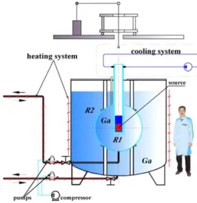
The Baksan Experiment on Sterile Transitions (BEST) is an experiment stationed at the Baksan Neutrino Observatory (BNO) designed to explore the gallium anomaly and search for the possible exis-tence of a fourth neutrino flavor. The BNO has 4700 m of water equivalent shielding overhead to protect against cosmic ray backgrounds [20]. BEST is a short-baseline neutrino oscillation experiment that uti-lizes an artificial, compact 3.28 MCi 51Cr source of nearly monochromatic electron neutrinos (751 keV,
90.12%) to irradiate two separate gallium targets at distances of ∼0.4 m and∼0.8 m, respectively [21]. The experimental layout is shown in Figure 2. The51Cr source used in the experiment has a half-life of
Figure 2: BEST experimental layout with average person shown for scale. The center vessel is spherically shaped with radiusR1 = 0.66 m. The outer vessel is cylindrically shaped with radius
R2 = 1.096 m and height = 2*R2. Both vessels are filled with homogeneous liquid gallium,71Ga.
The central region where the 51Cr source is located can be approximated as a sphere of radius
27.7 days, decaying through electron capture and primarily producing neutrinos with an energy of 747 keV, near the energy of neutrinos produced in the p-p chain. As the 51Cr source in the center of the apparatus irradiates the two target regions with νe, gallium is converted into germanium through the reaction
71Ga +ν
e→71Ge +e− (8)
This isotope of germanium is unstable and has a relatively short half-life of 11.43 days, decaying solely via electron capture to the ground state of 71Ga. It can be extracted through radiochemical methods
described in [22] in order to be counted as individual atoms through its decay products. The decay of
71Ge releases Auger electrons and x-rays with sum energies of 10.4 keV (K peak) or 1.2 keV (Lpeak),
both of which are measured using proportional counters filled with extracted gas containing the produced
71Ge [23].
The relatively short half-life of 51Cr forces the measurement cycle of the experiment to be 10
ex-tractions of 71Ge from the large gallium-filled vessels once every 9 days after initial installation of the
source. Each of the two containers are extracted from individually in order to allow for two simultaneous experiments to occur at two baseline distances. Under the gallium anomaly, best-fit values for ∆m2
41and
sin2(θe4) are found to be 2.3 eV2and 0.24, respectively. BEST is designed to probe the regions including
and around these parameters. The estimated sensitivities of the BEST experiment are shown in Figure 3.
Figure 3: Regions favored by the BEST experiment in the cases that: (left panel) it finds no anomaly or (right panel) it confirms the anomaly. These plots and descriptions of how these regions were determined can be found in [21].
Without oscillation into a sterile neutrino state, the mean production rate of71Ge in each vessel for
the first extraction is expected to be∼65 atoms per day. With a Monte Carlo simulation of the entire experiment, the rate in each zone was expected to be measured with a statistical uncertainty of about 3.7% with total systematic uncertainty of about 2.7% [21].
2.1
Proportional Counters
When the 71Ge is extracted from each separate vessel, it is synthesized into GeH
4 gas mixed with
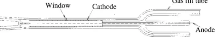
Xe and inserted into a very-low-background proportional counter (PC). A diagram of a PC is shown in Figure 4. These detectors rely on the phenomenon of gas multiplication to amplify charge from originally produced ion pairs. Electric fields of magnitude∼106 V/m between the cathode sleeve and anode wire
allow freede−to cause a Townsend avalanche toward the anode. This phenomenon results in a fractional increase in the number of free electrons falling toward the anode per unit path length dependent on the type of gas being used and the strength of the electric field. Thus, when electrons are freed from gas molecules through radioactive processes or particle collisions, they are amplified by a Townsend avalanche creating a signal at the anode proportional in magnitude to the initial energy of the freed electrons.
Figure 4: Diagram of an example proportional counter used in BEST. Total length from leftmost plug to the anode is approximately 10 cm with an 8 mm outer diameter. Sample gas is filled through the labeled gas fill tube. The window label indicates a hole in the counter body and cathode covered by a thin piece of brown silica to allow for x-ray transmission during calibration. Further description of PC design and fabrication can be found in [20].
lesser extent. Approximately the same number of events are expected to occur in the K andL peaks because of inefficiencies in x-ray observation, even thoughK peak events occur for over 80% of decays [20]. For71Ge events, most electrons from the cascade of electrons are expected to arrive very quickly at
the anode, followed by a smaller tail of the rest of the cascaded electrons being collected over a longer period of time. This is because the deposition of energy from71Ge events is considered point-like. When
the signal is processed through an analog-to-digital converter, this behavior takes on the form of a sharp rise in signal after pulse onset followed by a flattening out over the rest of the pulse’s duration. A sample pulse is shown in Figure 10.
To determine the energy of each signal, the integral of the pulse waveform for 800 ns after pulse onset is recorded for each event. To convert this value into its corresponding energy value, a55Fe source is used to calibrate the measurement. The nearly monochromatic 5.9 keV x-rays produced from this source are projected into the counter through the window in their side immediately after filling. Calibrations are performed after approximately 3 days of initial operation, and approximately every 2 weeks until the 6 months of its operation are completed. Because of the large flux of 5.9 keV events recorded during each calibration, a Gaussian fit to the mean ADC value of each data set taken during a calibration would correspond to an energy of 5.9 keV. Assuming a linear calibration between energy values, the ratios of theKandLpeak energies to the calibration energy, 10.4/5.9 and 1.2/5.9 respectively, would indicate the ADC position of each respective peak. Under this linear assumption, these ratios would also shrink or widen the measured standard deviation of the Gaussian fit to appropriately match the energy magnitude of each peak. Linear interpolation is also used between calibrations to determine the small changes in peak location that occurs over time.
2.2
Pulse Shape Discrimination
In addition to theKandLpeak events observed in each PC, there are also a number of background events recorded that are not of interest to the measurements made in this experiment. These events include cosmic ray-induced backgrounds,222Rn decay from natural radon which entered the PC during
filling or calibration, pulses that saturate the ADC, and HV breakdown events. For some of these events, tagging from other devices in the experiment or cutting time regions of data is possible to prevent them from being included in analysis. For many of them, however, these cuts are not possible and additional information is needed to discriminate background events from71Ge events.
To decide which events to include in the analysis and which to exclude, pulse shape discrimination (PSD) is used to differentiate between events of interest and background. Using features of event wave-forms is the most frequently used type of PSD. Auger electron events and x-ray depositions caused by the decay of71Ge are point-like energy depositions that create distinct pulse shapes when measured with PCs. For timetafter pulse onset, they are expected to follow a shape described by, fort > TN:
V(t) = V0
TN TN ln
t−ts+t0−TN
t0
−1
−(t−ts+t0)
ln
1− TN
t−ts+t0
+Voff (9)
and fort < TN:
V(t) = V0
TN
(t−ts+t0) ln
1 + t−ts
t0
−(t−ts)
+Voff (10)
whereV(t) describes the voltage input to a preamplifier at time t,Voff is the offset voltage point of the
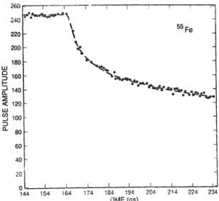
Figure 5: An example55Fe PC pulse fit to equations 9 and 10 is shown. Individual data points
are the sample pulse and the dashed line is the fit. The parameters used for this fit are V0 = -46
mV,t0 = 0.36 ns, andTN = 1.6 ns. The figure was borrowed from [24].
TN is the time over which the extended pulse drifts to the anode (measure of rise time of the waveform). Derivation of these equations and further description of their meaning is given in [24]. An example pulse fitted to these equations is shown in Figure 5. When fitting waveforms taken from real data to these equations, the best fit parameters can be used to demonstrate differences between71Ge events and
background events.
Point-like71Ge events are collected rapidly at the anode, leading to smaller rise-time,T
N, values. For true point ionization, this value is close to 0, meaning events with relatively largeTN values are likely background events such as a high-energyβ particle. This parameter is energy dependent because lower energy events take less time to collect, so limits are placed on the maximum allowable rise time for each of theKandLpeak events separately. This prevents events with high rise times from being included in analysis.
In addition to this rise time technique, the electronics configuration of the experiment measures an additional parameter: the amplitude of the differentiated pulse (ADP). This quantity is proportional to the product of the original pulse amplitude and the inverse rise time. Thus, if divided by the energy of the pulse (ADP/E), this parameter is also a good measure of the rise time for a particular waveform. Events with low ADP/E values have longer rise times and are likely background events. Events with very high ADP/E values have very short rise times and are likely breakdown or saturated events, and thus are also likely backgrounds. Careful selection of an appropriate window of ADP/E values can then eliminate many of these backgrounds effectively leading to better selection of the events of interest for the experiment. Descriptions of all PSD techniques for this section were taken from [20].
Although both of these rise time PSD techniques are fairly effective, they fail to use information stored in the entirety of the waveform, only observing specific features of each pulse and describing an event in terms of single parameters. If a new technique could be developed that used all information stored in a particular waveform, improvements could be made upon these techniques that would increase the precision and accuracy of waveform-based analyses. This improvement would not be exclusive to BEST, but would be applicable to any experiment which analyzes pulse signals and wants to differentiate backgrounds from candidate events. For these reasons, this study aims to test the viability of deep learning methods in achieving high quality PSD.
2.3
Data Set and Cuts
This data set is split into two kinds of data: calibration and physics. The calibration data contains all measurements taken during each calibration done for a particular PC over its 6 month counting period. The physics data contains all data taken over the 6 month counting period of a particular PC when the PC is kept within its purged passive shield. For this study, the calibration data sets are used for training and establishment of parameter cuts while the physics data sets are used for analysis.
In conjunction with data cuts made using the neural network (described in Section 3), additional cuts were made on the data set to remove contaminated events and events known to not be from the decay of71Ge. Because of the nature of energy calibration for the experiment, some of these cuts were
unable to be applied to calibration data, and thus only apply to physics data sets. All cuts, described in [20] and adjusted to their current usage in [17], include the following:
• Removal of all data 15 minutes prior and 3 hours subsequent to an event that saturates the energy scale of the ADC. This cut accounts for 222Rn contamination that entered the counter during filling. Rn decays that mimic those of 71Ge are always accompanied by 3α particles which are detected with high efficiency and which saturate the counter pulse. Thus, this cut removes any events corresponding to that particular decay.
• Removal of all high voltage breakdown events. These pulses have a very sharp pulse rise followed by a plateau and can be identified from the pulse slope between 500 and 1000 ns after pulse digitization begins.
• Removal of all data acquired within 2.6 hours of the opening of the passive shield surrounding the PC. Air surrounding the PCs within the passive shield is continuously purged with evaporating LN, but the PCs are exposed to counting room air when calibrated, which contains natural Rn. Thus, after resealing the Rn shield surrounding each PC following a calibration, time is given to allow for removal of the Rn from the surrounding air. This cut removes events which were possibly caused by the decay of Rn in the shield volume.
• Removal of all pulses coincident with an appropriate signal from the surrounding NaI detectors. These detectors account for events which originate outside of the counter, likely caused by external radiation or cosmic ray-induced events. Two parameters are used to measure whether the NaI detectors have been triggered, NaITDC and NaIE. For this analysis, only events with an NaITDC value below 1 or above 5000 and an NaIE value below 20 are allowed to pass the cut.
• Restriction of energy windows for theKandLpeaks. Using the calibration techniques mentioned in Section 2.1, the mean ADC values of each peak is chosen. All events within 1 FWHM (determined using the calibrated σ from the Gaussian fit) of the mean value pass this cut for each peak, respectively.
• Restriction of the rise time windows for each peak. Because rise time is energy dependent, theK
and Lpeaks each have different acceptance windows for pulse rise time. Using theTN parameter described in equations 9 and 10, events with TN values lower than 10.0 ns and energies within theL peak range, as well as events withTN values lower than 18.4 ns and energies within the K peak range are allowed to pass this cut. Events with higher rise times are cut and assumed to be background.
Because calibrations take place outside of the PC’s passive shielding, only NaI event cuts are applied to calibration data before using it for analysis. The vastly larger flux of55Fe events overwhelms all Rn-induced events in the PCs, so those cuts are not necessary, nor are they possible because of the opening of the passive shield. Each of the other cuts applies only to physics data.
3
Waveform Characterization with a Neural Network
networks are used to classify different kinds of events in data sets, observe features and trends in data sets that would otherwise go unnoticed, and automate a variety of analyses. The event classification and feature observation benefits of neural networks are of particular use in waveform analysis and PSD.
Neural networks are algorithms loosely modeled after the behavior of human brains that consist of several layers, each filled with a particular number of data points. Data points in the network are referred to as nodes or neurons. The first layer of the network is the input layer, consisting of one node for each data point being used to describe a particular event. In the case of waveform analysis, this layer consists of one node for each sample in a waveform.
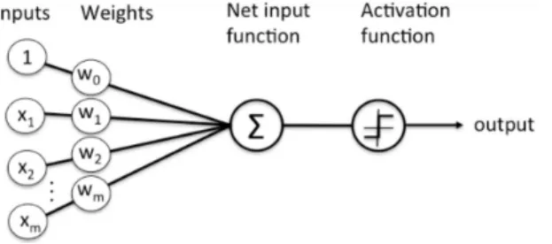
Layers subsequent to the input layer but prior to the output layer are known as hidden layers. The outputs of these layers are not observed, but they are crucial to the operation of the network and are the aspects of the network that change the size of the input data and notice trends in the data. To connect the input layer to the first hidden layer, every node in the hidden layer is connected to every input node through a system of weights. Each node in the hidden layer multiplies each of the values incident on it with a different coefficient. These coefficients are randomized when the network is first created and are adjusted as the network is trained to produce the best output possible. Once each incident value is weighted, they are all summed together at the node in the hidden layer. A visual diagram of how this occurs for one particular node is shown in Figure 6.
Figure 6: Example of how a node in a hidden layer operates. Inputs are weighted, summed, and passed through an activation function before creating the output of the node. Diagram taken from [28].
To determine the value that each of these hidden layer nodes will pass onto the next layer in the network, an activation function is assigned to each hidden layer. This function determines the extent to which a node is “turned on” based on the sign and magnitude of the summed value at the node. This is similar to the behavior of neurons in the brain, which fire only when stimulated to a certain extent. The most common examples of activation functions include (letf(x) be the output of the function and
xbe the summed value at the node):
• Linear- Uncommon activation function mostly used for output layers. Allows the summed value of the node to pass to the following layer regardless of its value. (f(x) =x)
• ReLU - Rectified Linear Activation Unit, the most commonly used activation function. Similar to the Linear function, but returns 0 for any summed node value ≤0. Used to observe nonlinear behavior in a data set without large amounts of computation. (f(x) =xfor x>0, 0 otherwise)
• Sigmoid- Another common activation function, normally used to lead to binary outputs. Output value between 0 and 1 is returned, large positive values yield outputs close to 1, large negative values yield outputs close to 0. This is a poor choice of activation function when large magnitude numbers are used. (f(x) =1+1e−x)
Each of these activation functions serve different purposes in helping to analyze the data from the input layer, with the ReLU activation function being used the most in hidden layers. Each hidden layer operates the same way following the first layer, taking all of the inputs of the previous layer, weighting them, and passing them through an activation function.
functions used for this layer are usually chosen very carefully also depending on the desired output. For example, a desired binary output would likely employ the sigmoid activation function to distinguish outputs as 0 or 1. For a quantitative description of input data in terms of multiple parameters, however, the ReLU or Linear activation functions are often used to preserve the magnitudes of the calculated results.
Neural networks can be designed any number of ways using these tools, each specific to the intended purpose of the network. Different numbers of layers, numbers of nodes, and types of activation functions are used to analyze the data from the input layer and produce an intended output. These structures are only half of how the network’s algorithm works, however, as the randomly instantiated weight coefficients must be adjusted to emphasize the important features of the input data. To adjust these values, neural networks must be trained on a set of data before they can be used.
3.1
Training
Once the structure of a neural network is established, it has to then be trained in order for it to perform its intended function. Training is similar to how neurons in the brain must learn to be activated in certain situations in order to accomplish specific functions. In the case of neural networks, nothing is changed about the structure of the network as it is trained. Only the weighting values used to magnify the significance of values from previous nodes are altered. There are two possible methods used to train neural networks: supervised and unsupervised learning.
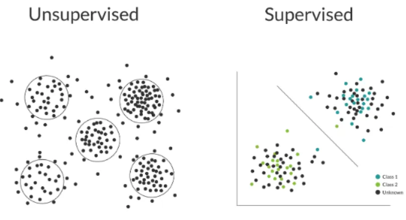
Supervised learning attempts to reduce the error between the network’s output and the desired output using a training data set with known output values. The network is provided with a large sample of input/output pairs and weights are altered between each node as each event in the sample is passed through the network to minimize the error between the determined and expected output. This method of training is often used for analyses that desire binary good/bad event outputs. The network would be given a data set filled with labeled good and bad events, often created through Monte Carlo simulations, in proportions similar to what would be expected from a real data set, and then train on each event in that set until it could reproduce the expected good/bad result after passing the event through the network as accurately as possible. A visual example of the result of this kind of training is shown in Figure 7. This method is extremely useful, but also has some flaws. Because the outputs of the training
Figure 7: Supervised vs Unsupervised learning example data sets. Supervised learning is used to distinguish pre-decided trends in data. Unsupervised learning is used to discover trends or clusters in a data set without being told what to look for specifically. Diagram taken from [29].
set are pre-known, the network learns to only observe features in the data set that lead to those outcomes and is unable to observe other features present in the data set. The second training method accounts for this.
parameters, and reproduces the input as accurately as possible. Through condensing and recreating the input data, the network is able to observe and determine what features make up the input data, thus observing trends in the data on its own without outside influence. A visual example of this is shown in Figure 7. The feature vector is then used as a description of the waveform condensed into much fewer parameters and the observed trends in these parameters can be used to analyze a data set. This is the type of learning used in this study.
Once the type of training is selected, the actual modification of the network must be performed. To adjust the randomized weights of a network, backpropagation is used as a means of improving the results of the output layer. To adjust weights in the network, the simplest version of the backpropagation algorithm operates as follows:
1. Weights for each layer in the network,W(n)where the boldface text indicates that it is a matrix
of weight values, are randomly initialized
2. For a data set withmsamples (consisting of a set of input-output pairs,X) and a network withn
layers, each sample (1 to m) performs the following:
(a) The initial sample is passed through each layer of the network. As it is passed through, the weighted sum and activation function output from each node, sn
j and anj, respectively, are saved. j represents the node in a particular layer
(b) The final output created from this pass-through is then used to determine the partial deriva-tives of a differentiable error function, E(X,W(n)), in terms of each input weight used to create the output value. The error function is a measure of the difference between the output of the network and the desired output, similar to a least-sqaures regression function. Evalua-tion of the error funcEvalua-tion is first done for only the last layer, and is then propagated backward through the network for each weight value using the previous value and the values saved in the forward pass-through of the network. Each partial derivative is saved as an error value, δn
j, for each node in the output layer until a matrix of error function gradients,∇W, is calculated with the same dimensions asW(n)
(c) Using each of these calculated values, a gradient descent step is taken for each weight in the network according to the matrix equation:
W(n+1)=W(n)−α∂E(X,W
(n))
∂W (11)
where αis a preset learning rate that determines how significant each weight change should be
(d) Each gradient descent step edits the weights of the network to produce an output closer in value to the desired output for given input values. The magnitude of how much each weight is changed depends on the preset rate of adjustment desired for altering weight values,α, and how effective the randomized weight values were when they were first created
3. After each of theminput-output pairs are passed through the backpropagation algorithm and the network is updated to better produce the desired outcome, a loss value is calculated using the error function, E, that quantifies the quality of the network’s performance. If the loss value is high, further training is necessary (either using the same data set or additional training data). If the loss value is low, the network accurately predicts the desired output values and can be used
A more complete and extensive description of this algorithm can be found in [30]. This simpler version, however, illustrates the basic principles behind how neural networks operate and are trained.
More complicated versions of the basic backpropagation algorithm follow a similar structure but employ additional methods. For the algorithm used in this study, the main additional features are adjustable optimizers, batch sizes, and epochs. Optimizers are used to alter the method used to adjust weights after error values are calculated. Instead of being restricted to only a gradient descent method of adjustments of weights, additional methods which use adaptive step sizes (learning rates) and account for past gradient steps to adjust weighting changes can be applied to the optimization of the network. This improves the convergence of the network to lower loss values and leads to faster, more accurate training.
larger batch size adjusts how many samples from a particular data set are observed before making an adjustment to the weights in the network. For small training sets, small batch sizes are required to increase the frequency of how the network is adjusted. For larger training sets, a larger batch size is needed so that the network can observe the general trends in the data before making an adjustment. Batches which pass randomly selected events from the training set are optimal for these larger batch sizes to ensure the network sees each kind of event in a particular data set and does not overtrain on one kind of event. Epochs control how many times the network passes through the complete data set when training. Because a single pass through a training set is often not enough to adjust the network’s parameters adequately, extra passes through the set give the optimizer extra opportunities to observe the necessary data trends and adjust accordingly. Choosing optimal values for each of these items is critical to ensuring that the network completes its training on a training set as a whole rather than only on a small portion of the set.
3.2
Autoencoders
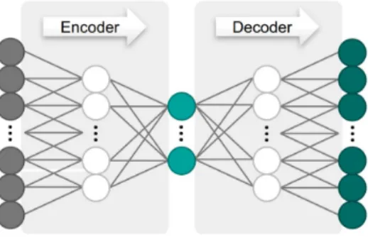
A neural network employing unsupervised learning over supervised learning was chosen to increase the background discrimination capabilities of this study. The best choice to observe trends in waveform shapes and behavior that could later be used to make background cuts was an autoencoder. This kind of neural network takes an input sample, in this case a signal pulse, reduces it down to a small feature vector (called the encoded representation) through several hidden layers, and extrapolates it back out to its original size. The extrapolated version is then compared to the input pulse and the network is trained to reproduce the input pulse as accurately as possible. The aspect of the network that condenses the sample down to its encoded representation is known as the encoder and the aspect of the network that reproduces the waveform from the small feature vector is known as the decoder. More accurate reproductions imply encoded representations of the waveform which better describe the features of the pulse. A diagram of how this occurs is shown in Figure 8.
Figure 8: Diagram of how a basic autoencoder operates. Consists of input layer, hidden layers used to condense the input layer into a smaller number of parameters, encoded representation of input (usually a small number of parameters depending on how many are necessary to reproduce the input data), hidden layers symmetric to the previous ones to expand the encoded representation back to the size of the input layer, and a reproduced output meant to be as similar to the input as possible. Diagram taken from [25].
3.2.1 Convolutional Autoencoders
Normal autoencoders are excellent for observing global trends in given samples due to their use of fully connected layers (layers whose nodes are connected to every node in the previous layer and every node in the following layer). For waveform analysis, however, it is often useful to be able to observe local trends in the pulse that distinguish its behavior from other pulses. The addition of convolutional layers to the more standard fully connected layers used in an autoencoder can help achieve this observation.
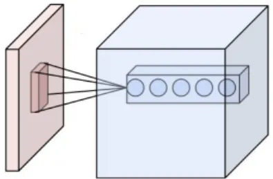
Unlike a fully connected layer, convolutional layers look at small regions of nodes in the previous layer. For a 1-dimensional input layer, each node along the width of the convolutional layer will look at a small number of nodes along the input. This node uses the same set of weights as a fully connected layer and can even have an activation function added, but is solely focused on a small region of the input layer. What makes convolutional layers even more unique, however, is the addition of depth to its layer. Each front node in the convolutional layer is backed by additional nodes with different weighting functions to search for different features of the same small input region. Thus, a 1-D input layer yields a 2-D convolutional layer with node depth. A 2-dimensional example of this is shown in Figure 9. The
Figure 9: Diagram of how a convolutional layer extracts information from a previous layer (2-D input layer example shown). There are a depth of nodes in the convolutional layer that are each connected to the same small region of nodes in the input layer. Each node in this depth searches for different features of the small region of input nodes using different weights. For each height and width position (just width position in a 1-D example) in the convolutional layer, there is the same depth of nodes that each search for the same set of different trends in different small regions of input nodes. Diagram taken from [31].
added depth of convolutional layers creates a moving window of sorts that is able to pick out different features of the same local region in a waveform. This is the advantage of using these kinds of layers.
The first node in the convolutional layer observes the first region of nodes in the previous layer, known as the receptive field of the convolutional layer’s node. Each node along the depth of that first convolutional layer node has the same receptive field, but a different set of weighting values to search for different features in the region. After each node along that depth calculates its respective value, the windows must move to the next region of the previous layer. To decide how this set of windows moves through the previous layer, the stride of the convolutional layer is specified along with its depth. Depth specifies how many windows are created in the convolutional layer to observe each receptive field. Stride specifies how many spaces the receptive field moves along the previous layer before it is analyzed by the next set of nodes. The stride of a convolutional layer is usually set to a value of 1 or 2 in order to observe as much of the previous layer as possible. [31]
Once a previous layer has been completely analyzed by a convolutional layer, the large convolutional layer must be shrunk to reduce the number of parameters describing the previous layer. This is ac-complished through pooling layers. Pooling layers look at small regions of previous layers, similar to convolutional layers, but do not analyze them with weighting functions. Instead, they choose the largest or smallest value in a region (depending on if it is a max pooling or min pooling operation) and use that as the new value describing the entire region of the previous layer. Without repeating the observation of any nodes in the previous layer, this operation shrinks the size of the convolutional layer while holding onto the most important bits of information from it. Thus it downsamples a previous layer while keeping in tact its information.
4
Analysis
4.1
BEST Network
Implementing all of these tools, a convolutional autoencoder was developed for data analysis particular to this study. This network is referred to as BEST Network, or BESTnet for shorthand.
BESTnet was developed using the high-level neural networks API, Keras [32], while running on top of a TensorFlow [33] backend in the programming language, Python. Versions used include Python 3.6.2, Keras 2.2.4, and TensorFlow 1.14.0. The network consists of 15 layers, including input and output, and has the following structure:
• Input Layer - Shape: 924 point waveform (first 100 points of original waveform removed to eliminate signal when multiplexer gate is open),Encoder beginning
• First Convolutional Layer - Shape: 916×30 array of nodes, Depth: 30, Stride: 1, Receptive Field Size: 9 nodes
• First Max Pooling Layer - Shape: 458×30 array of nodes (halves size of previous layer)
• Second Convolutional Layer - Shape: 454×15 array of nodes, Depth: 15, Stride: 1, Receptive Field Size: 5 nodes
• Second Max Pooling Layer- Shape: 227×15 array of nodes (halves size of previous layer)
• Third Convolutional Layer- Shape: 225×1 array of nodes, Depth: 1, Stride: 1, Receptive Field Size: 3 nodes
• Flattening Layer- Shape: 225 point set, removes second dimension added by convolutional layers so that fully connected layers can be used
• Fully Connected Layer - Shape: 100 point set, Activation Function: ReLU, reduces size of set from 225 to 100 points
• Fully Connected Layer - Shape: 5 parameter encoded representation, Activation Function: Linear, produces the encoded representation of the waveform,Encoder finish
• Fully Connected Layer- Shape: 100 point set, Activation Function: ReLU, expands the encoded representation back out to 100 points,Decoder beginning
• Fully Connected Layer- Shape: 219 point set, Activation Function: ReLU, continues to expand the set and reproduce the waveform
• Fully Connected Layer- Shape: 443 point set, Activation Function: ReLU, continues to expand the set and reproduce the waveform
• Fully Connected Layer- Shape: 916 point set, Activation Function: ReLU, continues to expand the set and reproduce the waveform
• Fully Connected Layer- Shape: 924 point set, Activation Function: Sigmoid, finishes expansion of the encoded representation and reproduces input waveform, Decoder finish
• Output Layer - Shape: 924 point waveform, finishes shaping details of the set (no weighting or activation functions) for comparison with input waveform
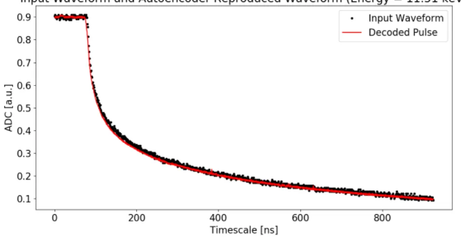
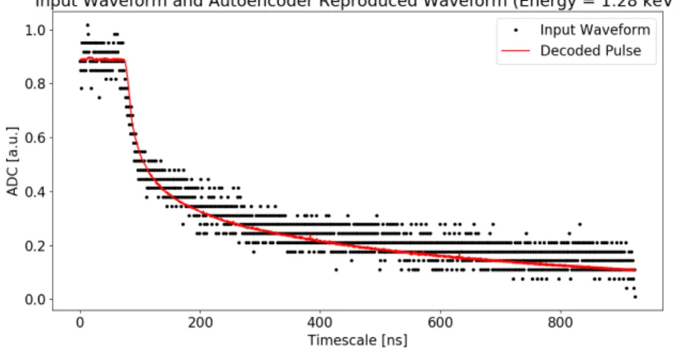
Figure 10: Example waveform and its autoencoder reproduction. This example pulse is taken from extraction 1401 (January 2014) calibration data. Because it is higher energy, the relative noise level of the pulse is low. The first 100 points of the 1024 point waveform are removed to eliminate signal when the multiplexer gate is open. The remaining baseline and pulse samples are normalized to fit between 0.1 and 0.9 to remove energy dependence from signal size.
waveform was desired. Because every input waveform is a set of data points normalized between 0.1 and 0.9, a sigmoid activation function was chosen to keep all output values between 0 and 1. The waveform reproduction capabilities of this network can be seen in Figure 10.
Every extraction involved in the 2014 SAGE data set used a different PC under different conditions, thus a different BESTnet was trained for each extraction. Each BESTnet had the same exact network structure, but different weighting values particular to each extraction.
Training of each extraction’s network was done using the full calibration data set from each extraction. At the start of each training, every other event in the calibration set (half of the total) was selected to be used for training with all other events being saved for testing of the network. This was done to get a variety of calibration events across the entire 6 month time period of the measurement in both the training and testing data sets. Of the events selected for training, 7.5% were randomly selected to be used as verification of the network’s performance while it was being trained. This was an additional option provided by Keras’s software that provided extra assurance of the quality of the network’s performance. In total, approximately 10,000 waveforms were used to train each network with an additional 10,000 used to test the network.
Every waveform in the 2014 data set consists of 1024 data points taken at 1 ns intervals. Approx-imately the first 200 of these data points are the signal when multiplexer gate is open and baseline of the waveform, with the following 800 creating the pulse itself. Description of the electronics system that triggers each event and records the pulse shape can be found in [20]. To remove the open multiplexer signal from this analysis and leave only the baseline and pulse shape, the first 100 points were cut from every waveform before use in a network. Additionally, to remove energy dependence based on pulse amplitude from network analysis, every waveform was normalized to exist between 0.1 and 0.9, giving them each the same amplitude. To do this, the first 20 data points and the last 10 data points of each waveform were averaged. The average of the last 10 points was then used to shift the entire waveform down to where the tail of the pulse flattened at a value of 0.1 [a.u.] and the average of the first 20 data points was used to scale the entire waveform to have a maximum amplitude of 0.9 [a.u.].
loss function in backpropagation applications because of its simplicity and simple differentiability. It is given by the equation:
MSE = 1
N
N
X
i=1
ˆ
Yi−Yi
2
(12)
whereN is the total number of samples being compared, ˆYi is the computed output value, andYiis the expected output value.
Each extraction’s BESTnet was trained using a batch size of 500 over 10 epochs. These values provided the most efficient and most accurate results after several trial tests. Additional epochs were not added beyond 10 because further changes to the loss values were insignificant beyond that number of epochs indicating possible overfitting of the data at further passes through the data.
12 networks in total were created and used in this analysis, one for each extraction in the 2014 SAGE data set. The full autoencoder network and the encoder half of the network were saved locally for each extraction after training. Upon completion of each training, the total loss value (error function final value) achieved for each network was on the order of e-4 using all aforementioned methods and structures. This considerably low loss value for training sets of approximately 10,000 waveforms indicates excellent reproduction of calibration waveforms through BESTnet. Figure 10 showcases this excellent performance through the clear reproduction of an input calibrated waveform. Figure 11 highlights the ability of the network to reproduce low energy pulse shapes which have much higher relative noise levels than higher energy pulses. Although not as precise as the higher energy waveform reproductions, low
Figure 11: Example low energy waveform and its autoencoder reproduction. This example pulse is taken from extraction 1401 (January 2014) physics data. The first 100 points of the 1024 point waveform are removed to eliminate signal when the multiplexer gate is open. The remaining baseline and pulse samples are normalized to fit between 0.1 and 0.9 to remove energy dependence from signal size.
energy waveform reproductions have a moderate degree of accuracy. These plots are indicative of the vast majority of reproduced waveforms from both calibration and physics data sets. Each epoch of training took approximately 10 s to complete while running on a local ThinkPad laptop (Intel Core i5 processor), resulting in an average training time near 100 s per extraction data set.
4.2
BESTnet Data Cuts
Figure 12: Example parameter distribution of calibration data from the third parameter of extraction 1401 (January 2014). The55Fe source used has a single energy peak at 5.9 keV clearly
shown through the grouping of data around that value. This distribution is indicative of the average distribution for all calibration data parameters. Center red line is the mean value from the Gaussian fit of the data for this parameter, upper and lower bounds are set 2σapart from the mean on each side. These 2σbounds were used to make cuts on physics data for this parameter of this extraction.
distributions behaved similar to this example, with mean values between -5 and 5 a.u. and standard deviations (σ) on the order of 0.1 a.u.
The clear grouping of values within∼1 keV of the 5.9 keV expected energy peak for55Fe demonstrates
the consistency of pulse shapes for those events. Because the calibration events are point-like, just as the products of71Ge events are expected to be, a fit of each parameter’s distribution should serve as a good
model of the expected parameter distribution for71Ge events. Thus, after processing the calibration test
data through its respective encoder, distributions of each parameter value are fit to a Gaussian function using the output. 2σ bounds on either side of the Gaussian mean for each parameter were saved to a .csv file to use as bounds for data cuts on physics data for that extraction. Using 2σbounds is slightly more restrictive than the 1 FWHM bounds used for energy cuts, but this was not found to significantly impact the results of the analysis. Bounds were created and saved in this manner for each of the five parameters used to describe waveforms in each respective data set.
This process was done for the following data sets from the complete SAGE 2014 data set: 1401, 1402, 1403, 1404, 1406, 1407, 1408, 1410, 1411A. The first two digits of the data set name represent the year in which the data were taken (2014) and the last two digits represent the month in which the extraction for that particular data set was performed (01 - January, etc.). Data sets 1405, 1409, and 1412 were left out of this analysis because of computational issues with determining data cuts for the parameters in each of these sets. Data set 1411 was split into two sets, A and B, because data were recorded over the course of 12 months rather than the usual 6 as a measure of experiment backgrounds once71Ge should
have decayed away. Only data set A was considered for this analysis to keep the 6 month measurement period consistent between data sets.
respective networks. Analysis of the correlation between parameters for separate networks trained on the same data set is planned as part of future work in order to achieve a better understanding of the features that BESTnet observes.
5
Results
The performance of BESTnet was evaluated based on an event-by-event comparison between the offi-cial event selection for 2014 data performed by SAGE and the event selection performed using BESTnet. Comparison is displayed for each extraction analyzed in this study separately and as a total percentage of agreement.
Figure 13: Example parameter distribution of physics data from the third parameter of extraction 1401 (January 2014). This distribution is indicative of the average distribution for all physics data parameters. Center red line is the mean value from the Gaussian fit of the calibration data for this parameter, upper and lower bounds are set 2σapart from the mean on each side.
BESTnet event selection was performed using the cuts described in Section 2.3 in conjunction with network creation, training, and application described in Section 4. The cuts from Section 2.3 were applied to physics data first to reduce the amount of waveforms which needed to be processed through BESTnet. The remaining data were then passed through its respective network and parameter cuts were applied to arrive at the final event list. An example plot showing how the BESTnet parameter cut shown in Figure 12 affected its set of physics data is shown in Figure 13. Each event outside of the cut bounds is eliminated from the final event list. This physics distribution and the effects of the parameter cuts are indicative of all other parameter distributions.
Two separate lists, one for K peak events and one for L peak events, were created and compared with the official event list to evaluate performance of the network at each energy involved in the BEST Experiment.
5.1
K
Peak Event List Comparison
An event-by-event comparison of K peak selected events was performed first because the improved signal-to-noise ratio of the experiment in this region should yield optimal performance. The results are shown in Table 2.
Extraction (Month) Official Number of Events BESTnet Number of Events Extra/Missing Events
1401 (Jan.) 14 13 1 missing
1402 (Feb.) 13 15 2 extra
1403 (Mar.) 12 12 None
1404 (Apr.) 7 8 1 extra
1406 (Jun.) 5 5 3 extra, 3 missing
1407 (Jul.) 9 11 2 extra
1408 (Aug.) 16 17 2 extra, 1 missing
1410 (Oct.) 13 16 3 extra
1411A (Nov.) 7 4 3 missing
Table 2: Kpeak candidate event list comparison for the extractions analyzed in this study from the 2014 SAGE data set.
set. At Los Alamos National Laboratory (LANL), study of this data set was conducted concurrently with the study described in this paper in order to also create a comparative event list. This study used more traditional data cuts, such as rise time and likelihood, to arrive at its event list. Although not the official BEST event list, the strong agreement between K peak results for this event list and the BESTnet created list suggest good performance of BESTnet in distinguishingKpeak candidate events. The large disagreement in the 1406 data set likely occurred as a result of lenient rise time (TN) cuts for theK peak as many of the extra events had large rise times very near where the cut was set for this analysis. Additionally, the events missing from this list and from the poor-agreement 1411A list had parameter values near the cut limits, so expansion of the parameter cut boundaries to 1 FWHM instead of 2σmay be able to solve that discrepancy. It is possible that each of these cut boundary changes may also fix discrepancies in the other lists.
Considering the 91.7% agreement between BESTnet’s list and events found in the official list, the acceptance of 13.5% more events, and the failure to accept 8.3% of official events, it is apparent that BESTnet performs fairly well for K peak discrimination of the decay of 71Ge. Improvements to the
performance of the network may be possible, but current performance in this energy region appears relatively adequate.
5.2
L
Peak Event List Comparison
An event-by-event comparison ofLpeak selected events was performed following theKpeak analysis to observe the performance of BESTnet in the low energy, high background region of the experiment. The results are shown in Table 3.
Extraction (Month) Official Number of Events BESTnet Number of Events Extra/Missing Events 1401 (Jan.) 16 12 5 extra, 9 missing 1402 (Feb.) 16 7 2 extra, 11 missing 1403 (Mar.) 21 6 5 extra, 20 missing 1404 (Apr.) 14 14 8 extra, 8 missing 1406 (Jun.) 9 6 3 extra, 6 missing 1407 (Jul.) 9 7 1 extra, 3 missing 1408 (Aug.) 23 12 9 extra, 20 missing 1410 (Oct.) 31 26 7 extra, 12 missing 1411A (Nov.) 22 12 5 extra, 15 missing
Table 3: Lpeak candidate event list comparison for the extractions analyzed in this study from the 2014 SAGE data set.
On average, each data set was missing 11.56 events and contained 5.00 additional events when com-pared to the official SAGE list determined from more traditional methods for the same data set. Of the 161 candidate events recorded by the official list, BESTnet was able to discriminate 57 of the same events, missing 104 events and recording 45 additional events.
well as non-linear BESTnet parameter behavior for lower energies. In Figures 12 and 13, there is clearly a more sparse distribution of parameter values for event energies below 3 keV. This is due to the low SNR in pulse shapes in this energy region. An example pulse in this energy range is shown in Figure 14. The magnitude of pulses in the low energy region is relatively small, resulting in very noisy signals
Figure 14: Example low energy waveform and its autoencoder reproduction. This example pulse is taken from extraction 1401 (January 2014) physics data. Although the reproduction of this waveform is fairly accurate, the low gain pulse is clearly a poor description of the true shape of this event. The individual ADC values are extremely visible for each point on the waveform, indicating poor relative precision for each data point in the pulse. Using high gain waveforms for this lower energy analysis is one method that would improve the precision of those individual values, and thus the network’s ability to reproduce the waveform.
that are fit relatively poorly (compared to higher energies) by BESTnet which only uses lower-resolution low gain waveforms. This could possibly be improved by training and testing BESTnet with high gain waveforms in this low energy region.
Considering the 35.4% agreement between BESTnet’s list and events found in the official list, the acceptance of 28.0% more events, and the failure to accept 64.6% of official events, it is apparent that BESTnet performs poorly with respect toLpeak discrimination of the decay of71Ge. Improvements to
parameter cuts made in this energy region will be necessary for BESTnet to be useful in determiningL
peak events.
5.3
Future Prospects
Although this study only presents a comparison between the performance of BESTnet and the results of more traditional methods, there is intent to investigate the performance of the network using a parameter that quantifies the discrimination power (ability to separate good and bad events) of the network in future research. This parameter would evaluate the performance of the network in each energy region and provide a more accurate description of BESTnet’s abilities. Time constraints prevent this parameter from being presently created and explored.
Additional future work related to BESTnet involves completing the analysis of remaining data sets and improving performance of the network at low energies. Completion of the analysis of the remaining 3 data sets will involve a period of code debugging that there was not time to complete prior to the completion of this report.
Improving performance of the network at lower energies could involve a variety of actions, such as investigating the time-dependence of mean parameter values as each run records data over 6 months, using hi gain waveforms to train additional networks for analysis of low energy events, and looking into the behavior of the wider parameter distributions of the current BESTnet at lower energies. Each of these options may or may not improve the performance of BESTnet at low energies, and they will each be looked into as a possible solution.
of waveforms produced from the decay of71Ge instead of training on55Fe events which are of a different energy. This could also improve BESTnet performance and event discrimination capabilities.
6
Conclusion
BESTnet was designed and tested successfully over the course of this study. Using a 15-layer con-volutional autoencoder, low gain waveforms from SAGE’s 2014 data set were able to be accurately reproduced and represented in the form of a 5 parameter feature vector. The parameter representation of each waveform was used, in conjunction with traditional physics background, energy, and rise time cuts, to remove background events from the data set and create a candidate event list of possibleK and
Lpeak events from the decay of 71Ge. TheK peak candidate event list was found to be in reasonable
agreement with the official BEST event list, while theLpeak candidate event list was found to be in poor agreement with the official BEST event list. With improvements to its performance at lower energies, these results indicate that BESTnet could be an effective form of pulse shape discrimination for the BEST experiment.
References
[1] Wolfgang Pauli. Open letter to the group of radioactive people at the gauverein meeting in t¨ubingen. letter, 1930.
[2] C. L. Cowan, F. Reines, F. B. Harrison, H. W. Kruse, and A. D. McGuire. Detection of the free neutrino: a confirmation. Science, 124(3212):103–104, 1956.
[3] Raymond Davis. A review of the homestake solar neutrino experiment. Progress in Particle and Nuclear Physics, 32:13 – 32, 1994.
[4] S Fukuda, Y Fukuda, M Ishitsuka, Y Itow, T Kajita, J Kameda, K Kaneyuki, K Kobayashi, Y Koshio, M Miura, et al. Solar 8B and hep neutrino measurements from 1258 days of super-kamiokande data. Physical Review Letters, 86(25):5651, 2001.
[5] SNea Ahmed, AE Anthony, EW Beier, Alain Bellerive, SD Biller, J Boger, Mark Guy Boulay, MG Bowler, TJ Bowles, SJ Brice, et al. Measurement of the total active8B solar neutrino flux at
the sudbury neutrino observatory with enhanced neutral current sensitivity. Physical review letters, 92(18):181301, 2004.
[6] M. et al. Tanabashi. Review of Particle Physics. Phys. Rev. D, 98:030001, Aug 2018.
[7] Carlo Giunti and Chung Wook Kim. Fundamentals of neutrino physics and astrophysics. Oxford University Press, 2007.
[8] A. Aguilar, L. B. Auerbach, R. L. Burman, D. O. Caldwell, E. D. Church, A. K. Cochran, J. B. Donahue, A. Fazely, G. T. Garvey, R. M. Gunasingha, and et al. Evidence for neutrino oscillations from the observation ofνeappearance in aνµ beam. Physical Review D, 64(11), Nov 2001.
[9] Sebastian Bser, Christian Buck, Carlo Giunti, Julien Lesgourgues, Livia Ludhova, Susanne Mertens, Anne Schukraft, and Michael Wurm. Status of light sterile neutrino searches. Progress in Particle and Nuclear Physics, page 103736, Nov 2019.