Linear Mathematics In Infinite Dimensions: Signals, Boundary Value Problems and Special Functions - Free Computer, Programming, Mathematics, Technical Books, Lecture Notes and Tutorials

(1)

LINEAR MATHEMATICS

IN

INFINITE DIMENSIONS

Signals

Boundary Value Problems

and Special Functions

U. H. Gerlach

January 2017

2nd Beta Edition

In its “2nd Beta Edition” this document is meant for private

or class room consumption. As such I ([email protected])

would appreciate feedback about the strengths as well as

weaknesses (e.g. lack of clarity, insufficient

(2)

Preface

Mathematics is the science of measurement, of establishing quantitative re-lationships between the properties of entities. The entities being measured occupy the whole spectrum of abstractness, from first-level concepts, which are based on perceptual data obtained by direct observation, to high-level concepts, which are further up in the edifice of knowledge. Furthermore, be-ing the science of measurement, mathematics provides the logical glue that cements and cross-connects the structural components of this edifice.

1. The effectiveness and the power of mathematics (and more generally of logic) in this regard arises from the most basic fact of nature: to be is to be something, i.e. to be is to be a thing with certain distinct properties, or: to exist means to have specific properties. Stated negatively: a thing cannot have and lack a property at the same time, or: in nature contradictions do not exist, a fact already identified by the father of logic1 _{some twenty-four}

centuries ago.

Mathematics is based on this fact, and on the existence of a consciousness (a physicist, an engineer, a mathematician, a philosopher, etc.) capable of identifying it. Thus mathematics is neither intrinsic to nature (reality), apart from any relation to man’s mind, nor is it based on a subjective creation of a man’s consciousness detached from reality. Instead, mathematics furnishes us with the means by which our consciousness grasps reality in a quantitative manner. It allows our consciousness to grasp, in numerical terms, the micro-cosmic world of subatomic particles, the macro-micro-cosmic world of the universe and everything in between2_{. In fact, this is what mathematicians are}

sup-1_{Aristotle, the Greek philosopher, 384-322 B.C.}

2_{The objectivity of mathematics and its relation to physics is explicated in “The Role}

of Mathematics and Philosophy”, Chapter 7, in THE LOGICAL LEAP: Induction in Physics by David Harriman (New York: Penguin Group, 2010).

(3)

posed to do, to develop general methods for formulating and solving physical problems of a given type.

In brief, mathematics highlights the potency of the mind, its cognitive efficacy in grasping the nature of the world. This potency arises from the mind ability to form concepts, a process which is made most explicit by the science of mathematics.3

2. Mathematics is an inductive discipline first and a deductive disci-pline second. This is because, more generally, induction preceeds deduc-tion4_{. Without the former, the latter is impossible. Thus, the validity of the}

archetypical deductive reasoning process

“Socrates is a man. All men are mortal. Hence, Socrates is a mortal.” depends on the major premise “All men are mortal.” It constitutes an iden-tification of the nature of things. It is arrived at by a process of induction, which, in essence, consists of observing the facts of reality, of identifying their essential properties, and of integrating them with what is already known into new knowledge – here, a relationship between “man” and “mortal”. In math-ematics, inductively formed conclusions, analogous to this one, are based on motivating examples and illustrated by applications.

Mathematics thrives on examples and applications. In fact, it owes its birth and growth to them. This is manifestly evidenced by the thinkers of Ancient Greece who “measured the earth”, as well as by those of the En-lightenment, who “calculated the motion of bodies”. It has been rightfully observed that both logical rigor and applications are crucial to mathemat-ics. Without the first, one cannot be certain that one’s statements are true. Without the second it does not matter one way or the other5_{. These lecture}

notes cultivate both. As a consequence they can also be viewed as an at-tempt to make up for an error committed by mathematicians through most

3_{Being a philosopher, Leonard Peikoff in his}_{Objectivism: The Philosophy of Ayn Rand}

(New York: Penguin books, 1993, p. 90) describes the role of mathematics this way:

“The mathematician is the exemplar of conceptual integration. He does professionally and in numerical terms what the rest of us do implicitly and have done ever since childhood, to the extent that we exercise our distinctive human capacity”.

4_{“The Structure of Inductive Reasoning”, Section 1.5, in}_{THE LOGICAL LEAP:} In-duction in Physics by David Harriman (New York: Penguin Group, 2010, p. 29-35).

5_{David Harriman, “Enlightenment Science and Its Fall”,}_{The Objective Standard;} _1(1):

(4)

iii

of history – the Platonic error of denigrating applications6_.

This Platonic error, which arises from placing mathematical ideas prior to their physical origin, has metastasized into the invalid notion ‘“pure” math-ematics’. It is a post-Enlightenment (Kantian) fig leaf7 _{for the failure of}

theoretical mathematicians to justify the rigor and the abstractness of the concepts they have been developing. The roots of this failure are expressed in the inadvertent confession of the chairman of a major mathematics depart-ment: “We are all Platonists in this department.” Plato and his descendants declared that reality, the physical world, is an imperfect reflection of a purer and higher mystical dimension with a gulf separating the two. That being the case, they aver that “pure” mathematics – and more generally the “ a priori” – deals only with this higher dimension, and not with the physical world, which they denigrate as gross and imperfect, and dismiss as mere appearances.

With the acceptance – explicit or implicit – of such a belief system, “pure” mathematics has served as a license to misrepresent theoretical mathematics as a set of floating abstractions cognitively disconnected from the real world. The modifier “pure” has served to intimidate the unwary engineer, physi-cist or mathematician into accepting that this disconnect is the price that mathematics must pay if it is to be rigorous and abstract.

Ridding a culture’s mind from impediments to epistemic progress is a non-trivial task. However, a good first step is to banish detrimental termi-nology, such as “pure” mathematics, from discourses on mathematics and replace it with an appropriate term such as theoretical mathematics. Such a replacement is not only dictated by its nature, but it also tends to reinstate the intellectual responsibility among those who need to live up to their task of justifying rigor (i.e. precision) and abstractness.

3. Mathematics is both complex and beautiful. The complexity of math-ematics is a reflection of the complexity of the relationships that exist in the universe. The beauty of mathematics is a reflection of the ability of the human mind to identify them in a unit-economical way8 _{: the more}

eco-6_ibid.

7_{more precisely, a rationalization, i.e. a cover-up, namely a process of providing one’s}

emotions with spurious justifications. (“Philosophic Detection” in Ayn Rand,Philosophy: Who Needs It, New American Library, Penguin Group Inc., New York, 1984.)

8_The _{principle of unit-economy} _{(also known informally as the “crow epistemology”)}

(5)

nomical the identification of a constellation of relationships, the more man’s mind admires it. Beauty is not in the eyes of the beholder. Instead it is giving credit where credit is due – according to an objective standard. In mathematics that standard is the principle of unit economy. Its purpose is the condensation of knowledge, from the perceptual level all the way to the conceptual at the highest level.

4. Linearity is as fundamental to mathematics as it is to our mind in forming concepts. The transition from recognizing thatx+y=x+y to the act of grasping thata+a= 2a is the explicit starting point of a conceptual consciousness grasping nature in mathematical terms with linearity at the center. Thus it is not an accident that linear mathematics plays its pervasive role in our comprehending the nature of nature around us. In fact, it would not be an exaggeration to say that “Linearity is the exemplary method – simple and primitive – for our grasping of nature in conceptual terms”. The appreciation of this fact is found in that nowadays virtually every college and university offers a course in linear algebra, with which we assume the reader is familiar.

5. Twentieth century mathematics is characterized by an inflationary version of Moore’s Law. Moore’s Law expresses the observation that the number of transistors that fit onto a microchip doubles every two years. This achievement has been a boon to everybody. It put a computer into nearly every household.

The mathematical version of Moore’s Law expresses the observation that, up to the Age of Enlightenment, all of Man’s mathematical achievements fit into a four-volume book; the achievements up to, say, 1900 fit into a fourteen-volume tome, while the mathematical works generated during the twentieth century take up a whole floor of a typical university library.

Such abundance has its delightful aspects, but it is also characterized by repetitions and non-essentials. This cannot go on for too long. Such an increase ultimately chokes itself off.

One day, confronted with an undifferentiated amorphous juxtaposition of mathematical works, a prospective scientist/engineer/physicist/mathematician might start wondering: “I know that mathematics is very important, but am I learning theright kind of mathematics?”

Such a person is looking for orientation as to what is essential, i.e. what is

(6)

v

fundamental, and what is not. It has been said that the value of a book9_{, like}

that of a definition10_{, can be gauged by the extent to which it spells out the}

essential, but omits the nonessential, which is, however, left implied. With that in mind, this text develops from a single perspective six mathematical jewels (in the form of six chapters) which lie at the root twentieth century science.

Another motivation for making the material of this text accessible to a wider audience is that it solves a rather pervasive problem. Most books which the author has tried to use as class texts either lacked the mathe-matics essential for grasping the nature of waves, signals, and fields, or they misrepresented it as a sequence of disjoint methods. The student runs the danger of being left with the idea that the mathematics consists of a set ofad hoc recipes with an overall structure akin to the proverbial village of squat one-room bungalows instead of a few towering skyscrapers well-connected by solid passage ways.

6. We extend and then apply several well-known ideas from finite dimen-sional linear algebra to infinite dimensions. This allows us to grasp readily not only the overall landscape but it also motivates the key calculations whose purpose is to connect and cross-link the various levels of abstraction in the constructed edifice. Even though the structure of these ideas have been developed in linear algebra, the motivation for doing so and then using them comes from engineering and physics. In particular, the goal is to have at one’s disposal the constellation of mathematical tools for a graduate course in elec-tromagnetics and vibrations for engineers or electrodynamics and quantum mechanics for physicists. The benefits to an applied mathematician is the acquisition of nontrivial mathematics from a cross-disciplinary perspective.

All key ideas of linear mathematics in infinite dimensions are already present with waves, signals, and fields whose domains are one-dimensional. The transition to higher dimensional domains is very smooth once these ideas have been digested. This transition does, however, have a few pleasant sur-prises. They come in the form of special functions, whose existence and prop-erties are a simple consequence of the symmetry propprop-erties of the Euclidean plane (or Euclidean three-dimensional space). These properties consist of the

9_{Question and answer period following “You and Your Research” by Richard Hamming.} http://www.cs.virginia.edu/~robins/YouAndYourResearch.html

Also see the Appendix, page 477.

(7)

invariance under translations and rotations of distance measurements and of the shapes of propagating waves.

7. What is the status of the concept “infinite” appearing in the title of this text? Quite generally the concept “infinite” is invalid metaphysically but valid mathematically.

In the sense of metaphysics (i.e. pertaining to reality, to the nature of things, to existence) infinity falls into the category of invalid concepts, namely attempts to integrate errors, contradictions, or false propositions into something meaningful. Infinity as a metaphysical idea is an invalid concept because metaphysically it is only concretes that exist, and concretes are finite, i.e. have definable properties. An attempt to impart metaphysical significance to infinity is an attempt to rewrite the nature of reality.

However, in mathematics infinity is a well defined concept. It has a def-inite purpose in mathematical calculations. It is a mathematical method which is made precise by means of the familiar δ-ε process of going to the limit. This text develops only concepts which by their nature are valid. In-cluded is the concept “infinity”, which, properly speaking, refers to a math-ematical method.

8. The best way to learn something is to teach it. In order to facilitate this motto of John A. Wheeler, the material of this book has been divided into fifty lecture sessions. This means that there is one or two key ideas between “Lecture n” and “Lecture n + 1”, where n = 1,_{· · ·}50. Often the distance betweenn andn+ 1 extends over more pages than can be digested in a forty-eight minute session. However, the essentials of the nth Lecture are developed in a small enough time frame. Thus the first four or five pages following the heading “Lecturen” set the direction of the development, which is completed before the start of lecture “Lecturen+ 1”.

Such a division can be of help in planning the schedule necessary to learn everything.

9. It is not necessary to digest the chapters in sequential order. A de-sirable alternative is to start with Sturm-Liouville theory (chapter 3) before proceeding systematically with the other chapters. Moreover, there is obvi-ously nothing wrong with diving in and exploring each chapter according to one’s background and predilections. The opening remarks of each one point out how linear algebra relates it to the others.

(8)

vii

multiresolution analysis.

Ulrich H. Gerlach Columbus, Ohio, March 24, 2009

Foreword to the Second Edition (

tentative

₎

TBD

Mathematics is the language of Physics. Why?

Mathematics is beautiful. Why? Is its beauty in “the eyes of the be-holder”? Is beauty an attribute intrinsic to mathematics? Or is it an objec-tive attribute?

(9)

(10)

Chapter 0 Introduction

Lecture 1

The main focus of the next several chapters is on the mathematical frame-work that underlieslinear systems arising in physics, engineering and applied mathematics. Roughly speaking, we are making a generalization from the theory of linear transformation onfinite dimensional vector space to the the-ory of linear operators oninfinite dimensional vector spaces as they occur in the context of homogeneous and inhomogeneous boundary value and initial value problems.

The key idea is linearity. Itsgeometrical imagery in terms of vector space, linear transformation, and so on, is a key ingredient for an efficient compre-hension and appreciation of the ideas of linear analysis to be developed. Thus it is very profitable to repeatedly ask the question: What does this correspond to in the case of a finite dimensional vector space?

Here are some examples of what we shall generalize to the infinite dimen-sional vector case:

I. Solve each of the following linear algebra problems 1. A~u= 0 “Homogeneous problem”

2. A~u=~b “Inhomogeneous problem” 3. AG=I “Inverse ofA”

These are archetypical problems of linear algebra. (If 1. has a non-trivial solution, then 2. has infinitely many solutions or none at all, depending on ~b, and 3. has none.)

(17)

More generally we ask: For what values of λ do the following have a solution (and for what values do they not):

1. (A−λB)~u= 0 2. (A−λB)~u=~b 3. (A₋λB)G=I

Of greatest interest to us is the generalization in which A is (part of) a differential operator with in general non-constant coefficients.

As we know from linear algebra, these three types of problems are closely related, and consequently this must also be the case for our generalization to linear differential equations, ordinary as well as partial. In fact, these three types are called

1. Homogeneous boundary or initial value problems; 2. Inhomogeneous problems;

3. Green’s function problems.

II. There is another idea which we shall extend from the finite to the infinite dimensional case. Consider the eigenvalue equation

Au=λIu .

Let us suppose that there are enough eigenvectors to span the whole vector space, but that at least one eigenvalue is degenerate, i.e., it has more than one eigenvector. In that case, the vector space has an eigenbasis, but it is not unique. Eigenvectors, including those used for a basis, derive their physical and geometrical significance from eigenvalues. Indeed, eigenvalues serve as labels for eigenvectors. Consequently, the lack of enough eigenvalues to distinguish between different eigenvectors in a particular eigensubspace introduces an intolerable ambiguity in our physical and geometrical picture of the inhabitants of this subspace.

In order to remedy this deficiency one introduces another matrix, say T, whose eigenvectors are also eigenvectors ofA, but whose eigenvalues are non-degenerate. The virtue of this introduction is that the matrix T recognizes explicitly and highlights, by means of its eigenvalues, a fundamental physical and geometrical property of the linear system characterized by the matrixA. This explicit recognition is stated mathematically by the fact that T commutes withA

(18)

3

In general, the matrixT is not unique. Suppose there are two of them, say T1, which highlights property 1 andT2, which highlights a different property

of the system. Thus

AT1−T1A= 0

and

AT2−T2A= 0,

but

T1T2−T2T1 6= 0.

Consequently, for hermitian matrices, the matrix A is characterized by two alternative orthonormal eigenbases, one due to T1, the other due to T2, and

there is a unitary transformation which relates the two bases.

The matrix A does not determine the choice of eigenbasis. Instead, this choice is determined by which of the two physical properties we are told to (or choose to) examine, that of T1 or that ofT2.

In the extension of these ideas to differential equations, we shall find that

A = Laplace operator T1 = translation operator

T2 = rotation operator

and that the T1-induced eigenbasis consists of plane wave solutions, the T2

-induced eigenbasis consists of the cylinder wave solutions, and the unitary transformation between them is a Fourier transform.

III.A further idea which these notes extend to infinite dimensions is that of an inhomogeneous four-dimensional system,

A~u=~b ,

which is overdetermined: the matrix A is 4×4, but singular with a one-dimensional null space.

The extension consists of the statement that (a) this equation is a vec-torial wave equation which is equivalent to Maxwell’s field equation, (b) the four-dimensional vectors ~u and~b are 4-d vector fields, and (c) the matrix A has entries which are second order partial derivatives.

(19)

functions. For Maxwell’s equations there are exactly three of them, and they are the scalars from which one obtains the three respective types of Maxweell fields,

• transverse electric (TE), • transverse magnetic (TM),

• transverse electric magnetic (TEM).

(20)

Chapter 1 Sturm-Liouville Theory

Lecture 2

1.1 Three Archetypical Linear Problems

We shall now take our newly gained geometrical familiarity with infinite dimensional vector spaces and apply it to each of three fundamental problems which, in linear algebra, have the form

1. (A₋λB)~u = 0

2. (A−λB)G=I

3. (A₋λB)~u =~b,

i.e., the eigenvalue problem, the problem of inverting the matrix A−λB, and the inhomogeneous problem.

The most important of these three is the eigenvalue problem because once it has been solved, the solutions to the others follow directly.

Indeed, assume that we found for the vector space a basis of eigenvectors, say

{~u1, . . . , ~uN}

as determined by

A~u=λB~u

(21)

(We are assuming that the matrices A and B are such that an eigenbasis does indeed exist.) In that case, the solutions to problems 2 and 3 are given by

G=

N

X

i=1

~ui~uHi

λi−λ

and

~u=

N

X

i=1

~uih~ui,~bi

λi−λ

respectively, as one can readily verify. Here~uH

i refers to the Hermitian adjoint

of the vector~ui.

On the other hand, suppose we somehow solved problem 2 and found its solution to be

G=Gλ.

Then it turns out that the complex contour integral of that solution, namely

1 2πi

I

Gλdλ=− N

X

i=1

~ui~uHi ,

yields the sum of the products

−

N

X

i=1

~ui~uHi

of the eigenvectors ~ui (i = 1, . . . , N) of the eigenvalue problem 1. Thus

solving problem 2 yields the solution to problem 1. It also, of course, yields the solution to problem 3, namely

~u =G~b .

Thus, in a sense, problem 1 and problem 2 are equally important.

(22)

1.2. THE HOMOGENEOUS PROBLEM 7

This will be done in the next chapter. There we shall also formulate and solve the inhomogeneous boundary value problem corresponding to problem 3.

We extend problems 1-3 to infinite dimensions by focussing on second order linear ordinary differential equations and their solutions. They are the most important and they illustrate most of the key ideas.

It is difficult to overstate the importance of Sturm-Liouville theory. Not only does it provide a practical means for dealing with those phenomena (namely wave propagation and vibrations) that underly twentieth century science and technology, but it also provides a very powerful way of reasoning which deals with the qualitative essentials, and not only with the quantitative details.

A Sturm-Liouville eigenvalue problem gives rise to eigenfunctions. It is extremely beneficial to view them as basis vectors which span an inner product space. Doing so places the theory of linear d.e.’s into the framework of Linear Algebra, thus yielding an easy panoramic view of the field. In particular, it allows us to apply our geometrical mode of reasoning to the Sturm-Liouville problem.

1.2 The Homogeneous Problem

The most basic linear problem consists of finding the null space of

A~u= 0.

The simplest nontrivial extension to differential equations consists of the homogeneous boundary value problem based on the second order differential equation

d2

dx2 +Q(x, λ)

d

dx +R(x, λ)

u(x) = 0

where a < x < b and λ is a parameter, with one of the following end point conditions:

1. u(a) = 0 Dirichlet conditions u(b) = 0

(23)

3. αu(a) +α′u′(a) = 0 βu(b) +β′_u′_{(b) = 0}

Mixed D. and N. conditions

4. u(a)−u(b) = 0 u′_(a)₋_u′_{(b) = 0}

Periodic boundary conditions

More generally one has

B1(u) ≡ α1u(a) +α′1u′(a) +β1u(b) +β1′u′(b) = 0

B2(u) ≡ α2u(a) +α′2u′(a) +β2u(b) +β2′u′(b) = 0,

which are the most general end point conditions as determined by the given α’s, α′_’s, _{β’s, and} _β′_{’s, which are} _{constants. These two boundary conditions} B1 and B2 are supposed to beindependent, i.e., there do not exist any

non-zero numbers c1 and c2 such that

c1B1(u) +c2B2(u) = 0 ∀u(x).

By contrast, if there does exist a non-zero solutionc1 andc2 to this equation,

then B1 and B2 are dependent.

Question: Can one give a clear vector space formulation of B1(u) = 0

B2(u) = 0

in terms of subspaces?

Question: What geometrical circumstance is expressed by “independence”? Answer: The vector 4-tuples {α1, α′1, β1, β1′} and {α2, α′2, β2, β2′} point into

different directions.

Question: What, if any, is the (or a) solution to the homogeneous boundary value problem?

Answer: The general solution to the d.e. is

u(x) = eu1(x, λ) +f u2(x, λ)

where e and f are integration constants. Let us consider the circumstance where u(x) satisfies the mixed D.-N. boundary conditions (3.) at each end point. These conditions imply

(24)

1.2. THE HOMOGENEOUS PROBLEM 9

and

0 = e[βu1(b, λ) +β′u′1(b, λ)] +f[βu2(b, λ) +β′u′2(b, λ)].

The content of the square brackets is known because ui(x, λ), α, α′, and

β, β′ _{are known or given. The} _unknowns _are _e _and _f_{, or rather their ratio.} Note that the trivial solution

e=f = 0⇔u(x) = 0 ∀x

is always a solution to the homogeneous system. Our interest lies in a non-trivial solution. For certain values ofλ this is possible. This happens when

0 = D(λ) =

[αu1(a, λ) +α′u′1(a, λ)] [αu2(a, λ) +α′u′2(a, λ)]

[βu1(b, λ) +β′u′1(b, λ)] [βu2(b, λ) +β′u′2(b, λ)] .

Values of λ, if any, satisfying D(λ) = 0 are called eigenvalues.

KEY PRINCIPLE: A differential equation is never solved until boundary conditions have been imposed.

We note that the allowed value(s) of λ, and hence the nature of the solution is determined by these boundary conditions.

Example (Simple vibrating string): Solve u′′+λu= 0 subject to the boundary conditions

u(a, λ) = 0 u(b, λ) = 0 .

Solution: Two independent solutions to the d.e. are u1(x) = sin

√ λx u2(x) = cos

√ λx . Consequently, the solution in its most general form is

u(x) = esin√λx+fcos√λx .

The boundary conditions yield two equations in two unknowns:

(25)

In order to obtain anontrivial solution, it is necessary that

0 =

sina√λ cosa√λ sinb√λ cosb√λ

or

sin(a₋b)√λ= 0 which implies

λn =

πn a₋b

2

n = 1,2, . . . .

Note thatn = 0 yields a trivial solution only. Why? Negative integers yield nothing different, as seen below.

What are the solutions corresponding to each λn? The boundary conditions

demand thate be related to f, namely, esinapλn+fcosa

p

λn= 0 ,

or

f =₋esina √

λn

cosa√λn

. Thus

u(x) = e cosa√λn

(cosapλnsin

p

λnx−sina

p

λncos

p

λnx)

or

un(x) =cnsin

p

λn(x−a) .

Here we have introduced subscriptn to distinguish the solutions associated with the different allowed values

λn =

nπ a₋b

2

n = 1,2, . . . .

The negative integers give nothing new. (Why?)

Comment: Forn = 0, i.e. λ= 0, there does not exist a non-trivial solution. Why? Because the application of the boundary conditions to the n = 0 solution,

u(x) = ex+f yields only e=f = 0.

(26)

1.3. STURM-LIOUVILLE SYSTEMS 11

a

b

x

u

₂

1

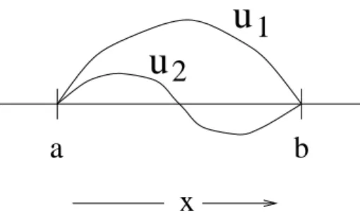
Figure 1.1: First two eigenfunctions of an eigenvalue problem based on Dirichlet boundary conditions.

1.3 Sturm-Liouville Systems

One of the most important and best understood eigenvalue problems in linear algebra is

(A₋λB)u= 0,

whereAis a symmetric matrix andB is a symmetric positive definite matrix. For this problem we know that

1. its eigenvalues form a finite sequence ofreal numbers

2. the eigenvectors form aB-orthogonal basis for the vector space; in other words,

UT

i BUj =δij.

A Sturm-Liouville system extends this eigenvalue problem to the frame-work of 2nd _{order linear ordinary differential equations (o.d.e.’s) where the}

vector space is infinite dimensional, as we shall see.

1.3.1 Sturm-Liouville Differential Equation

One of the original purposes of the Sturm-Liouville differential equation is the mathematical formulation of the vibration frequency and the amplitude profile of a vibrating string. Such a string has generally a space dependent tension and mass density:

T(x) = tension [force] ρ(x) = density

mass length

(27)

x

v(x,t)

Figure 1.2: Instantaneous amplitude profile of a suspended cable with vari-able tension and varivari-able mass density.

A cable of variable mass density, sayρ(x), suspended vertically from a fixed support is a good example. Because of its weight, this cable is under variable tension, sayT(x), along its length. Letv(x, t) be the instantaneous transverse displacement of the string.

Application of Newton’s law of motion, mass×acceleration=force, to the mass ρ(x)∆x of each segment ∆x leads to the wave equation for the trans-verse amplitude v(x, t),

ρ(x)∂

2_{v(x, t)}

∂t2 =

∂ ∂xT(x)

∂v(x, t) ∂x .

The force (per unit length) on the right hand side is due to the bending of the cable. Suppose the cable is imbedded in an elastic medium. The presence of such a medium is taken into account by augmenting the force density on the right-hand side. Being linear in the amplitude v(x, t), the additional restoring force density [force/length] is

−k(x)v(x, t) .

Herek(x)∆xis the position dependent Hooke’s constant experienced by the cable segment ∆x. Consequently, the augmented wave equation is

ρ(x)∂

2_{v(x, t)}

∂t2 =

∂ ∂xT(x)

∂v(x, t)

(28)

have vibrational frequencies ω and amplitudes v(x, t) =u(x) cosω(t₋t0).

Thus the spatial amplitude profile u(x) of such a mode satisfies

d dxT(x)

d

dx +λρ(x)−k(x)

u(x) = 0, λ=ω2. (1.2)

For the purpose of mathematical analysis one writes this 2nd _{order linear}

o.d.e. in terms of the standard mathematical notation

p(x) = T(x) ρ(x) = ρ(x) q(x) = k(x) ,

and thereby obtains what is known as the Sturm-Liouville (S-L) equation1_,

d dx

p(x)du dx

+ [λρ(x)₋q(x)]u= 0.

However, it is appropriate to point out that actually any 2nd _{order linear}

o.d.e. can be brought into this “Sturm-Liouville” form. Indeed, consider the typical 2nd _{order homogeneous differential equation}

P(x)u′′+Q(x)u′+ (R(x) +λ)u= 0.

We wish to make the first two terms into a total derivative of something. In that case, the d.e. will have its S-L form. To achieve this, divide by P(x) and then multiply by

eRx QPdt =p(x).

1_{The minus sign in front of} _q₍_x_{) is a reflection of the fact that the S-L equation had}

its origin in the mathematization of vibrating systems. There

₁

2p(u

′₎2₊1

2qu

2

dx

is the total potential energy stored in a string element of width dx: 1 2pu

2 _{is the bending}

energy/length and 1 2qu

2_{is the energy/length stored in the string due to having pushed by}

(29)

The result is

eRx QPdtu′′+ Q

Pe

Rx Q Pdtu′ +

R Pe

Rx Q Pdt+ λ

Pe

Rx Q Pdt

u= 0 or

p(x)u′′+p′(x)u′+ (λρ(x)₋q(x))u= 0

in terms of newly defined coefficients. Combining the first two terms one has

d dx

p(x)du dx

+ [λρ(x)₋q(x)]u= 0. (1.3)

This is known as theSturm-Liouville equation. In considering this equation, we shall make two assumptions about its coefficients.

The first one is

ρ(x) > 0 p(x) > 0

in the domain of definition, a < x < b. We make this assumption because nature demands it in the problems that arise in engineering and physics.

The second assumption we shall make is that the coefficients q(x), ρ(x), p(x) and p′_{(x) are continuous on} _{a < x < b. We make this assumption} be-cause it entails less work. It does happen, though, that p′_(x), _{q(x), or} _ρ(x) are discontinuous. This usually expresses an abrupt change in the propa-gation medium of a wave, for example, the tension or the mass density of string, or the refractive index in a wave propagation medium. This disconti-nuity can be handled by applying “junction conditions” for u(x) across the discontinuity.

1.3.2 Homogeneous Boundary Conditions

We can now state the S-L problem. If the endpoint conditions are of the mixed Dirichlet-Neumann type,

αu(a) +α′u′(a) = 0 (1.4) βu(b) +β′u′(b) = 0 ,

(30)

If, by contrast,

u(a)₋u(b) = 0 and p(a) =p(b) (1.5) u′_(a)₋_u′_{(b) = 0}

then Eqs.(1.3) and (1.5) constitute a periodic Sturm-Liouville system. Ifp(a) = 0 and the 1st_{b.c. in Eq.(1.4) is dropped, then we have a}_singular _S-L

system. We shall consider the properties of these S-L systems in a subsequent section.

It is difficult to overstate the pervasiveness of these S-L systems in nature. Indeed, natural phenomena subsumed under the regular S-L problem, for example, are quite diverse. Heat conduction and the vibration of bodies illustrate the point.

A. Heat conduction in one dimension.

Consider the temperature profile u(x) of a conducting bar of unit length which is

1. insulated at x= 0 (no temperature gradient), and satisfies 2. radiative boundary condition at x= 1

Separation of variables applied to the heat equation yields the following S-L system:

u′′+λu= 0 (1.6)

with

u′(0) = 0 (1.7)

−u′(1) = hu(1). (1.8)

Here h is a non-negative constant. Note that at x= 1

h = 0 _⇒ no radiation

h >0 _⇒ finite heat loss due to radiation (Newton’s law of cooling).

B. Vibrations in one dimension.

(31)

1. At x = 0 there is no transverse force to influence the string’s motion. The tension produces only a longitudinal force component. In this circumstance the string is said to be free atx= 0. This free boundary condition is expressed by the statement

u′(0) = 0 .

2. At x = 1 the string is tied to a spring so that the vertical spring displacement coincides with the displacement of the string away from equilibrium. Even though the tail end of the string gets accelerated up and down, the total transverse force on it vanishes because it has no mass. Consequently,

−u′(1)T −ku(1) = 0 , or

−u′(1) = hu(1) , where

h= k T =

spring constant string tension

The transverse amplitude profile of the string is governed by Eq.(1.2). For constant tension and uniform mass density this equation becomes

u′′+λu = 0

We see that the S-L system for the heat conduction problem, Eqs.(1.6)- (1.8), coincides with that for the vibration problem.

The task of solving this regular S-L system consists of findingall possible values ofλ for which the solution u(x, λ) is non-trivial. Consequently, there are four distinct cases to consider:

(32)

We shall have to consider cases 1.-3. only. This is because the next subsection (1.3.3) will furnish us with some very powerful theorems about the nature of the allowed values of λ and the corresponding non-trivial solutions u(x, λ).

1. λ = 0 leads tou=c1 +c2x

h >0 _⇒ c1 =c2 = 0 i.e., u(x) = 0 for all 0 < x <1

h= 0 _⇒ u(x) = c1

constant solution. (What physical circumstance is expressed byu(x) = c1?)

2. λ =α2 _>_0, _{α >}₀

The general solution to the differential equation is

u(x) = c1cosαx+c2sinαx .

Now consider the boundary conditions.

(a) Eq.(1.7) _⇒c2 = 0. Consequently,u(x) =c1cosαx .

(b) Eq.(1.8) _{⇒ −}αc1sinα+hc1cosα = 0. Consequently,

tanα = h

α. (1.9)

This transcendental equation determines the allowed values of α and hence of λ. How do we find them? A very illuminating way is based on graphs. Draw the two graphs (Figure 1.3)

y= tanα and

y= h α.

Where they intersect gives the allowed values of α, and hence λ=α2_,

the eigenvalues of the S-L problem. We see that there are an infinite number of intersection points

(33)

α

π 3π 5π 7π −π

2 2 2 2 2

αh tan α

Figure 1.3: There are two graphs in this figure: that oftan αand that of the two hyperbolash/α. The intersection of these two graphs is the solution set to the transcendental eigenvalue Eq.(1.9). The α-values of the heavy dots are the desired solutions. Note that if α is a solution, then ₋α is another solution, but it yields the same eigenvalueλ=α2_.

For largen we have αn≃(n−1)π. The correspondingeigenvalues are

λn =α2n n = 1,2,3,· · · .

Comment: One important question is this: how do the allowed eigen-values and eigenfunctions depend on boundary conditions? More on that later.

3. λ=−β2 _<₀_._{This leads to the general solution}

u(x) =c1coshβx+c2sinhβx .

The boundary conditions yield

tanhβ =₋h β .

(34)

4. What about complex λ?

We shall see in the next section that the eigenvalues of a S-L problem are necessarily real.

Lecture 4

1.3.3 Basic Properties of a Sturm-Liouville Eigenvalue

Problem

It is surprising how much useful information one can infer about the eigenval-ues and eigenfunctions of a S-L problem without actually solving the differ-ential equation explicitly. Thus from very general and simple considerations we shall discover that the eigenvalues are real, are discrete if the domain is finite, have a lowest member, increase without limit, and that the cor-responding eigenfunctions are orthogonal to each other, oscillate, oscillate more rapidly the larger the eigenvalue, to mention just a few pieces of useful information.

In practice this kind of information is quite often the primary thing of interest. In other words, the philosophy quite often is that one verifies that a certain system is of the S-L types, thus having at one’s immediate disposal a concomitant list of properties of the system, properties whose qualitative nature is quite sufficient to answer the questions one had about the system in the first place.

As promised, we shall develop these and other properties by means of a collection of theorems. But before doing so, we remind ourselves about what is meant by a “Sturm-Liouville system”, by a “solution”, and by “orthogo-nality”. The Sturm-Liouville system we shall consider consists of (i) the S-L differential equation

d dxp(x)

d

dx +λρ(x)−q(x)

u(x) = 0, (1.10)

whereq,ρ,p, andp′ _{are continuous and}_ρ_and_p_{are positive definite functions} on the open interval (a, b) together with (ii) the boundary conditions

(35)

where the given constants α, α′_, _β _and _β′ _are _{independent of the parameter} λ.

Corresponding to aneigenvalue of this S-L system, aneigenfunctionun(x)

is understood to be that solution which is “regular”, i.e.,

un(x) and

dun(x)

dx are continuous

and hence finite, on the closed interval [a, b]. In particular, an eigenfunction must not have any finite jump discontinuities anywhere in [a, b].

Orthogonality, Reality, and Uniqueness

Two eigenfunctionsum(x) andun(x) are said to beorthogonal relative to the

weight functionρ(x) if

Z b

a

um(x)un(x)ρ(x)dx= 0 whenever m6=n .

They are said to be orthonormal with respect toρ(x) if

Z b

a

um(x)un(x)ρ(x)dx=δmn. (1.12)

With these reminders at hand, one can now identify the two most impor-tant properties of a S-L system, the orthonormality of its eigenfunctions and the reality of its eigenvalues. The statement and the proof of these properties parallel those of the familiar eigenvalue problem from linear algebra,

A~u =λB~u

whereA is a Hermitian and B is a positive definite matrix.

Theorem 1 (Orthogonality) Let λm and λn be any two distinct eigenvalues

of the S-L problem 1.10 and 1.11 with corresponding eigenfunctions um and

un. Then um and un are orthogonal with respect to the weight ρ(x).

Orthogonality also holds in the following cases

(36)

2. when p(b) = 0 and the second (2) of the conditions 1.11 is dropped. This is equivalent to setting β=β′ _{= 0}

3. when p(a) =p(b) and 1.11 are replaced by

u(a) = u(b) (1.13)

u′(a) = u′(b) .

Remarks:

1. In case (1.) or (2.), the S-L problem is said to be singular.

2. The S-L problem with mixed Dirichlet-Neumann conditions at both ends is said to be regular.

3. The same terminology, (“singular”) is also used when

ρ(x) vanishes at an endpoint, q(x) is singular at an endpoint, (a, b) is unbounded.

In other words, we are not interested in the actual value of u(x), just that it staysfinite. This is sufficient to select (a multiple of the correct) one of two independent solutions to the differential equation.

4. The boundary conditions 1.13 are those of aperiodic S-L problem, for example, the one where x is the angle ϕ in cylindrical coordinates. (More on that later.)

5. This theorem is analogous to the orthogonality _hum, Buni = 0, of the

eigenvectors um and un of the familiar eigenvalue problem A~u=λB~u.

6. The physical significance of the orthogonality of the eigenfunctions is exemplified by the energy of a vibrating system governed by, say the wave equation, Eq.(1.1). Its total energy,

T.E.= 1 2

Z b

a

"

ρ(x)

∂v ∂t

2

+T(x)

∂v ∂x

2

+k(x)v2

#

dx , (1.14)

(37)

medium in which the string makes its transverse excursions. Performing an integration by parts on the second term, dropping the endpoint terms due to the imposed homogeneous boundary conditions, and using the governing wave equation, Eq.(1.1), one finds that the total energy is

T.E. = 1 2 Z b a " ρ(x) ∂v ∂t 2 +

−_∂x∂ T(x)∂v

∂x +k(x)v

v # dx = 1 2 Z b a " ∂v ∂t 2 − ∂ 2_v

∂t2v #

ρ(x)dx

Suppose the total vibrational amplitude is a superposition of the am-plitudes associated with with each eigenfrequency ωn,

v(x, t) = X

n

cnun(x) cos(ωnt+δn) .

Then the total energy becomes

T.E. = 1 2

X

m

X

n

[ωmωnsin(ωmt+δm) sin(ωnt+δn)

+ ωm2 cos(ωmt+δm) cos(ωnt+δn)

¯ cmcn

Z b

a

¯

um(x)un(x)ρ(x)dx

The orthonormality, Eq.(1.12), implies that

T.E.= 1 2

X

n

ω_n2_|cn|2 .

Thus we see that the orthonormality of the S-L eigenfunctions ex-presses the fundamental fact that the total energy, a constant inde-pendent of time, is composed of the mutually exclusive and constant energies residing in each normal mode (“vibratory degree of freedom”).

Proof in 3 Steps: In analogy to Aum = λmBum and Aun = λnBun one

first considers

Step (1)₋(pu′_m)′+qum

| {z }

k Lum

=λmρum; −(pu′n)′+qun

| {z }

k Lun

(38)

Then multiply the equations respectively by un and um and subtract

them. The left hand side becomes

l.h.s. = unLum−umLun≡

d

dxp(umu ′

n−unu′m) (1.15)

We now interrupt the three-step proof to remark that this is an important identity known as Lagrange’s Identity. We shall meet it and refer to it in several subsequent sections. This identity generalizes to higher dimensions by means of the vector identityun∇2um−um∇2un=∇ ·(un∇~um−um∇~un).

The integral version of Lagrange’s Identity is known as Green’s identity

Z b

a

(unLum−umLun)dx=p(x)(umu′n−unu′m)

b

a

(1.16)

in 1 dimension. Observe the parallel of this with Green’s Identity in three dimensions:

Z Z Z

volume

(un∇2um−um∇2un)d3x=

Z Z

boundary

(un∇~um−um∇~un)·dS .~

We now continue the three-step proof by considering the right hand side of the above subtraction result,

r.h.s.= (λm−λn)ρumun.

Step (2) Both sides are equal. Upon integrating them, one obtains

(λm−λn)

Z b

a

umunρ(x)dx=p(x)W[um, un](x)

b

a

where

W[um, un] =

um u′m

un u′n

.

This would be called theWronskian of um and un if λm and λn were equal.

(39)

Step (3a)If one has D-N conditions

αu(a) +α′u′(a) = 0 βu(b) +β′_u′_{(b) = 0}_, then these D-N conditions imply

W(a) = 0 W(b) = 0

because 1st _{= 2}nd _{columns are proportional. Thus for a} _regular _{S-L problem}

(λm−λn)

Z b

a

um(x)un(x)ρ(x)dx= 0,

i.e., one hasorthogonality whenever λm 6=λn.

Step (3b) If one has aperiodic S-L problem p(b) =p(a)

u(a) = u(b) u′_{(a) =} _u′_(b)

⇒W(a) =W(b).

i.e., one again hasorthogonality whenever λm 6=λn.

Setp (3c)If one has a singular S-L problem p(b) = 0

W(b) = finite

⇒p(b)W(b) = 0.

Similar considerations at the other end point also yield zero. Once again one has orthogonality whenever λm 6= λn. To summarize, the eigenfunctions of

different eigenvalues of regular, periodic, and singular Sturm-Liouville sys-tems are orthogonal.

Lecture 5

Theorem 2 (Reality of Eigenvalues) For a regular, periodic, and singular S-L system the eigenvalues are real.

Proof: Step (1) Let u be an eigenfunction corresponding to the complex eigenvalue λ =µ+iν. The eigenfunctions are allowed to be complex. Thus

(40)

because

L=L, ρ(x) =ρ(x) α, α′ ₌_{α, α}′

β, β′ ₌_{β, β}′

 



are real.

Step (2) We have, therefore,

Z b

a

(uLu−uLu)dx

| {z }

0 =p(x)W[u, u]

b

a

= (λ−λ)

Z b

a

uuρ(x)dx

0 = (λ₋λ)

Z b

a |

u_|2ρ(x)dx .

This implies that λ=λ, i.e., that λ is real.

We now inquire as to the number of independent eigenfunctions corre-sponding to each eigenvalue. This is a question ofuniqueness. The examples on page 15 have only one such eigenfunction for each eigenvalue. Consider, however, the following

Example (Periodic S-L system)

u′′+λu = 0 −1< x <1 u(₋1) = u(1)

u′(₋1) = u′(1).

We note that p(−1) = p(1). Consequently, this is a periodic S-L system. The form of the solution can be written down by inspection. Letting λ =α2_{, one obtains}

u(x) =c1cosαx+c2sinαx

without loss of generality we assume α > 0. The two boundary conditions imply

2c2sinα = 0

and

(41)

Both conditions yield non-zero solutions whenever α = 0, π,2π, . . .. Conse-quently, the eigenvalues are

λn=n2π2 n= 0,1,2,· · · .

Note that for every eigenvalue (exceptλ0) there are two eigenfunctions

λ0 :

1 2

λ1 : cosπx , sinπx

...

λn : cosnπx , sinnπx .

Such nonuniqueness is expressed by saying that each of the eigenvalues λ1, λ2, . . . is degenerate, in this example doubly degenerate because there are

two independent eigenfunctions for each eigenvalue.

The next theorem states that this cannot happen for a regular S-L system. Its eigenvalues are simple, which is to say they are nondegenerate.

Note that the theorem below uses Abel’s Theorem, namely Theorem 4. Theorem 3(Uniqueness of solutions to the regular S-L system.) An eigen-function of a regular Sturm-Liouville system is unique except for a constant factor, i.e., the eigenvalues of a regular S-L problem are simple.

Proof: For the same eigenvalue λ, let u1 and u2 be two eigenfunctions of

the regular S-L system. For a regular S-L system the b.c. are

αu1(a) +α′u′1(a) = 0

αu2(a) +α′u′2(a) = 0.

In other words, both solutions satisfy the D-N mixed boundary conditions at the left hand endpoint. The value of the Wronskian at x=a is

W[u1, u2](a) =

u1 u′1

u2 u′2

x=a

= 0,

columns are proportional

.

Using Abel’s Theorem: p(x)W[u1, u2](x) = constant, we obtain

u′ 1(x)

u1(x) −

u′ 2(x)

u2(x)

= 0_⇒u1(x) =ku2(x).

This conclusion says that the solution u1(x) is unique (up to a constant

(42)

NOTE:If the endpoint condition had been the periodic boundary condition, then one cannot conclude that the eigenvalues are simple. This is because

u(a) =u(b)

u′_{(a) =}_u′_(b) doesnot imply [u1(x)u′2(x)−u′1(x)u2(x)]x=a= 0.

The previous uniqueness theorem used Abel’s theorem, which applies to a second order linear differential equation regardless of any boundary conditions imposed on its solutions.

Theorem 4 (Abel) If u1 and u2 are two solutions to the same differential

equation

− d dxp

d dx +q

u=λρu (i.e., Lu=λρu), then

p(x)[u1(x)u′2(x)−u2(x)u′1(x)] = constant. (1.17)

Remark. The expression in square brackets, W =u1u′2−u2u′1

is called the “Wronskian” or the “Wronskian determinant”. Proof: Start with Lagrange’s identity

u2Lu1−u1Lu2 =

d dxp(u1u

′

2−u2u′1)≡

d

dxp(x)W[u1, u2].

Use the given differential equation to conclude that the left hand side van-ishes, i.e.

0 = d

dxp(x)W[u1, u2].

Thus p(x)W[u1, u2](x) is indeed a constant, independent of x.

A nice application of this theorem is that it gives us a way of obtaining a second solution to the given differential equation, if the first one is already known.

Using Abel’s theorem, the Wronskian determinant can be rewritten in the form

u2₁

u′ 2

u1 −

u2

u′ 1

u2 1

(43)

or

u2₁ d dx

u2

u1

= const. p . Integration yields the following

Corollary (Second solution)

u2 =u1(x)

Z x _dx_′

p(x′_)u2 1(x′)

+c1u1.

Thus one is always guaranteed a second solution if a first solution is known.

Exercise 1.3.1 (SCHR ¨ODINGER FORM: NO FIRST DERIVATIVES)

(a) SHOW that any equation of the form

u′′+b(x)u′+c(x)u= 0

can always be brought into the Schr¨odinger form (”no first derivatives”)

v′′+Q(x)v= 0

Apply this result to obtain the Schr¨odinger form for

(b)

u′′₋2xu′+λu= 0 (HERMITE EQUATION)

(c)

x2u′′+xu′+ (x2₋ν2)u= 0 (BESSEL’S EQUATION) (d)

xu′′+ (1−x)u′+λu= 0 (LAGUERRE’S EQUATION)

(e)

(1−x2)u′′−xu′+α2u= 0 (TSHEBYCHEFF’S EQUATION) (f)

(pu′)′+ (q+λr)u= 0 (STURM-LIOUVILLE EQUATION)

(g)

1 sinθ

d

dθ sinθ

d

dθ +ℓ(ℓ+ 1)−

m2

sin2_θ

(44)

Exercise 1.3.2 (NONDEGENERATE EIGENVALUES)

Consider the S-L eigenvalue problem

[Lun](x)≡

− d

2

dx2 +x

2

un(x) =λnun(x) ; lim

x→±∞u(x) = 0 ; (1.18)

on the infinite interval (_−∞,_∞).

Show that the eigenvalues λn are nondegenerate, i.e. show that, except for a

constant multiplicative factor, the corresponding eigenfunctions are unique.

Nota bene:

(i) The eigenfunctions are known as the Hermite-Gaussian polynomials. They are known to professionals in Fourier optics who work with laser beams passing through optical systems. A laser beam which is launched with cross-sectional amplitude profile un(x) one focal length away from a lens, passes

through the lens, and is then observed (on, say, a screen) one focal length after that lens, has an amplitude profile identical to the initial profileun(x).

(ii) These eigenfunctions are also known to physicists who work with simple har-monic oscillators (e.g. vibrating molecules), in which case the eigenfunctions are the quantum states of an oscillator and the eigenvalues are its allowed energies.

Exercise 1.3.3 (EVEN AND ODD EIGENFUNCTIONS)

Consider the “parity” operatorP :L2(_−∞,_∞)_→L2(_−∞,_∞) defined by

P ψ(x)_≡ψ(₋x)

(i) For a given function ψ(x), what are the eigenvalues and eigen functions of

P?

(ii) Show that the eigenfunctions of the operator L defined by Eq.(1.18) are eigenfunctions of P. Do this by first computing

P−1LP ψ(x)

forψ∈L2(−∞,∞) and then pointing out how P−1LP is related toL. Next point out how this relationship applied to an eigenfunction un of the

previous problem leads to the result P un=µun.

Exercise 1.3.4 (EIGENBASIS OF THE FOURIER TRANSFORM F)

Consider the S-L eigenvalue problem

[Lun](x)≡

− d

2

dx2 +x

2

un(x) =λnun(x) ; lim

(45)

on the infinite interval (_−∞,_∞). We know that the eigenvalues arenondegenerate

and are

λn= 2n+ 1, n= 0,1, . . . .

Consider now the Fourier transform onL2₍_−∞_,_∞_):

F[u](k)_≡

Z _∞

−∞

e−ikx

√

2πu(x)dx .

(a) By computing

FLF−1ψ(k)ˆ

for arbitrary ˆψ_∈L2₍_−∞_,_∞_{), determine the Fourier representation}

FLF−1 ≡L .ˆ of the operator

L=− d

2

dx2 +x

2

(b) By viewing F as a mapL2(−∞,∞)→L2(−∞,∞), compare the operators ˆ

Land L.

State your result in a single English sentence and also as a mathematical equation.

(c) Use the result obtained in (b) to show that each eigenfunctionunof the S-L

operatorLis also an eigenfunction of_F:

Fun=µ un.

By applying the result (e) of the Fourier eigenvector Exercise on page 149 to the previous Exercise determine the only allowed values forµ. What is

the Fourier transform of a Hermite-Gauss polynomialun(x)?

CONGRATULATIONS, you have just found an orthonormal eigenbasis of the Fourier transform operator F (in terms of the eigenbasis of the S-L operatorL)!

Exercise 1.3.5 (HOW TO NORMALIZE AN EIGENFUNCTION)

Consider the S-L system

d

dxp

d

dx −q+λρ

u= 0 a < x < b

(46)

Let w(x, λ) be that unique solution to _dxdpdw_dx + (λρ₋q)w = 0 which satisfies

αw(a, λ) +α′w′(a, λ) = 0. i.e. it satisfies the left hand boundary condition. Then

wn(x) ≡ w(x, λn) is an eigenfunction of the above S-L system corresponding to

the eigenvalue λn.

Calculate the normalization integral

b R a

w2

n ρ dxas follows:

(a) Obtain the preliminary formula

(λ₋λn) Z b

a

wn(x)w(x, λ)ρ(x)dx=p(b)W(w, wn)|x=b .

(b) By taking the limitλ→λn show that Z b

a

w_n2 ρ dx=p(b)

"

w′_n(b)dw(b, λ) dλ

λ=λn

−wn(b)

d

dλw′(b, λ)

λ=λn

#

,

where prime denotes differentiation w.r.t. x.

Exercise 1.3.6 (ORTHONORMALIZED BESSEL FUNCTIONS)

Consider the Sturm-Liouville (S-L) problem

− d dx x d dx + ν2 x

u=λxu .

Here u, du

dx bounded as x→0,u(1) = 0 whereν is a real number.

(a) Using the substitutiont=√λ x,show that the above differential equation reduces to Bessel’s equation of order ν. One solution which is bounded as t→ 0 is Jν(t); a second linearly independent solution, denoted by Yν(t), is

unbounded as t→0.

(b) Show that the eigenvalues λ1, λ2, . . . of the given problem are the squares

of the positive zeroes of Jν(

√

λ),and that the corresponding eigenfunctions are

un(x) =Jν( p

λn x) .

(c) Show that the eigenfunctions un(x) satisfy the orthogonality relation

1

Z

0

(47)

(d) For the caseν = 0, apply the method of the previous problem toexhibit the set of orthonormalized eigenfunctions{u0(x), u1(x), u2(x),· · · }.

(e) Determine the coefficients in the Fourier-Bessel series expansion

f(x)=.

∞

X n=1

cn un(x).

Exercise 1.3.7 (ORTHOGONALITY OF LEGENDRE POLYNOMIALS)

Consider the S-L problem

−_dxd (1₋x2) d

dx +

m2

1₋x2

u=λu

Here u, du

dx bounded as x → ±1. Here m = integer. The solutions to this S-L problem are un =Pnm(x), the “associated Legendre polynomials”, corresponding

toλn=n(n+ 1), n= integer. Show that

1

Z

−1

P_nm(x)P_nm′(x) dx= 0 λn6=λn′.

Lecture 6

Sturm’s Comparison Theorem

When confronted with the regular boundary value problem

d dxp(x)

d

dx −q(x) +λρ(x)

u(x) = 0 (1.19)

αu(a) +α′u′(a) = 0 (1.20) βu(b) +β′u′(b) = 0

we must ask

(48)

2. Why do the values of λ permitted by (1.19) and (1.20) form adiscrete and semi-infinite sequence

λ0 < λ1 <· · ·< λn<· · ·

with a smallest eigenvalue λ0 and with λn → ∞ as n→ ∞?

The “oscillatory nature” of a solution u(x, λ) is expressed qualitatively by the location of the zeroes of its graph. One could also inquire about its behaviour between successive zeroes. However, we shall see that such an inquiry always leads to the same answer: Provided q(x) +λρ(x) is positive between a pair of successive zeroes, the graph of u(x;λ) has only a single maximum (or minimum). This means that u(x, λ) cannot oscillate between two of its successive zeroes.

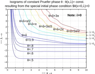
Thus the most important issue is the existence and location of the zeroes, which are controlled entirely by the phase of a given solution u(x, λ). This phase is a scalar function from which one directly constructs the solution. It is preferrable to discuss the behavior of the solution u(x;λ) in terms of its phase because the key qualitative properties of the latter are very easy to come by. As we shall see, one only needs to solve a first order differential equation, not the second order S-L equation.

However, before establishing and solving this differential equation, let us use the second order S-L differential equation directly to determine how the zeroes of u(xλ) are affected if the parameter λ is changed. We express this behaviour in terms of the

Sturm Comparison Theorem:

Wheneverλ1 < λ2, then between two zeroes of the nontrivial solutionu(x, λ1),

there lies a zero of u(x, λ2).

This theorem demands that one compare the two different solutions

u(x, λ1)≡u1(x) and u(x, λ2)≡u2(x)

of Eq. 1.19 corresponding two different constants λ1 and λ2. The conclusion

is obtained in three steps:

Step 1: Multiply these two equations respectively by u2 and u1, and then

form their difference. The result, after cancelling out the q(x)u1u2 term, is

d dx

p(x)

u2

du1

dx −u1 du2

dx

(49)

u(x,

λ

₁

)

u(x,

λ

₁

)

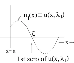
ζ

u (x)

1st zero of

x= a

1 x

Figure 1.4: Graph of a solutionu(x, λ1) which satisfies the mixed D-N

bound-ary condition at x=a.

which is the familiar Lagrange identity, Eq.(1.15), in disguise. Upon inte-gration one obtains

p(x)(u2u′1−u1u′2)

x

a

= (λ2 −λ1) Z x

a

u1u2ρ dx .

If bothu1 and u2 satisfy the mixed Dirichlet-Neumann boundary conditions

αu(a) +α′_u′_{(a) = 0 at} _x₌_{a, then}

(u2u′1−u1u′2)x=a=−

α

α′[u2(a)u1(a)−u1(a)u2(a)] = 0.

Ifx=a is a singular point of the differential Eq.(1.19),p(a) is zero. Thus, if uandu′_{are finite at}_x₌_{a, then the left hand side vanishes again at the lower} limit x = a. Thus both for a regular and for this singular Sturm-Liouville problem we have

p(x)

u2(x)

du1(x)

dx −u1(x)

du2(x)

dx

= (λ2−λ1) Z x

a

u1u2ρ dx .

Linear Mathematics In Infinite Dimensions: Signals, Boundary Value Problems and Special Functions - Free Computer, Programming, Mathematics, Technical Books, Lecture Notes and Tutorials