Computational Physics
With Python
Contents
Preface . . . vi
0 Useful Introductory Python 1 0.0 Making graphs . . . 1
0.1 Libraries . . . 5
0.2 Reading data from files . . . 6
0.3 Problems . . . 9
1 Python Basics 13 1.0 The Python Interpreter . . . 13
1.1 Comments . . . 14
1.2 Simple Input & Output . . . 16
1.3 Variables . . . 19
1.4 Mathematical Operators . . . 27
1.5 Lines in Python . . . 28
1.6 Control Structures . . . 29
1.7 Functions . . . 34
1.8 Files . . . 39
1.9 Expanding Python . . . 40
1.10 Where to go from Here . . . 43
1.11 Problems . . . 44
2 Basic Numerical Tools 47 2.0 Numeric Solution . . . 47
2.0.1 Python Libraries . . . 55
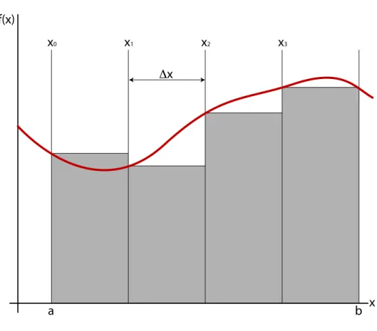
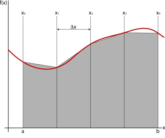
2.1 Numeric Integration . . . 56
2.2 Differentiation . . . 66
3 Numpy, Scipy, and MatPlotLib 73
3.0 Numpy . . . 73
3.1 Scipy . . . 77
3.2 MatPlotLib . . . 77
3.3 Problems . . . 81
4 Ordinary Differential Equations 83 4.0 Euler’s Method . . . 84
4.1 Standard Method for Solving ODE’s . . . 86
4.2 Problems with Euler’s Method . . . 90
4.3 Euler-Cromer Method . . . 91
4.4 Runge-Kutta Methods . . . 94
4.5 Scipy . . . 101
4.6 Problems . . . 106
5 Chaos 109 5.0 The Real Pendulum . . . 110
5.1 Phase Space . . . 113
5.2 Poincar´e Plots . . . 116
5.3 Problems . . . 121
6 Monte Carlo Techniques 123 6.0 Random Numbers . . . 124
6.1 Integration . . . 126
6.2 Problems . . . 129
7 Stochastic Methods 131 7.0 The Random Walk . . . 131
7.1 Diffusion and Entropy . . . 135
7.2 Problems . . . 139
8 Partial Differential Equations 141 8.0 Laplace’s Equation . . . 141
8.1 Wave Equation . . . 144
8.2 Schr¨odinger’s Equation . . . 147
8.3 Problems . . . 153
A Linux 155 A.0 User Interfaces . . . 156
A.1 Linux Basics . . . 156
CONTENTS v
A.3 File Ownership and Permissions . . . 162
A.4 The Linux GUI . . . 163
A.5 Remote Connection . . . 163
A.6 Where to learn more . . . 165
A.7 Problems . . . 166
B Visual Python 169 B.0 VPython Coordinates . . . 171
B.1 VPython Objects . . . 171
B.2 VPython Controls and Parameters . . . 174
B.3 Problems . . . 176
C Least-Squares Fitting 177 C.0 Derivation . . . 178
C.1 Non-linear fitting . . . 181
C.2 Python curve-fitting libraries . . . 181
C.3 Problems . . . 183
Preface: Why Python?
When I began teaching computational physics, the first decision facing me was “which language do I use?” With the sheer number of good program-ming languages available, it was not an obvious choice. I wanted to teach the course with a general-purpose language, so that students could easily take advantage of the skills they gained in the course in fields outside of physics. The language had to be readily available on all major operating systems. Finally, the language had to befree. I wanted to provide the students with a skill that they did not have to pay to use!
It was roughly a month before my first computational physics course be-gan that I was introduced to Python by Bruce Sherwood and Ruth Chabay, and I realized immediately that this was the language I needed for my course. It is simple and easy to learn; it’s also easy toread what another programmer has written in Python and figure out what it does. Its whitespace-specific formatting forces new programmers to write readable code. There are nu-meric libraries available with just what I needed for the course. It’s free and available on all major operating systems. And although it is simple enough to allow students with no prior programming experience to solve interesting problems early in the course, it’s powerful enough to be used for “serious” numeric work in physics — and it is used for just this by the astrophysics community.
Chapter 0
Useful Introductory Python
0.0
Making graphs
Python is a scripting language. A script consists of a list of commands, which the Python interpreter changes into machine code one line at a time. Those lines are then executed by the computer.
For most of this course we’ll be putting together long lists of fairly com-plicated commands —programs— and trying to make those programs do something useful for us. But as an appetizer, let’s take a look at using Python with individual commands, rather than entire programs; we can still try to make those commands useful!
Start by opening a terminal window.1 Start an interactive Python ses-sion, with pylab extensions2, by typing the command ipython−−pylab fol-lowed by a return. After a few seconds, you will see a welcome message and a prompt:
In [1]:
Since this chapter is presumbly about graphing, let’s start by giving Python something to graph:
In [1]: x = array([1,2,3,4,5]) In [2]: y = x+3
1In all examples, this book will assume that you are using a Unix-based computer:
either Linux or Macintosh. If you are using a Windows machine and are for some reason unable or unwilling to upgrade that machine to Linux, you can still use Python on a command line by installing the Python(x,y) package and opening an “iPython” window.
2All this terminology will be explained eventually. For now, just use it and enjoy the
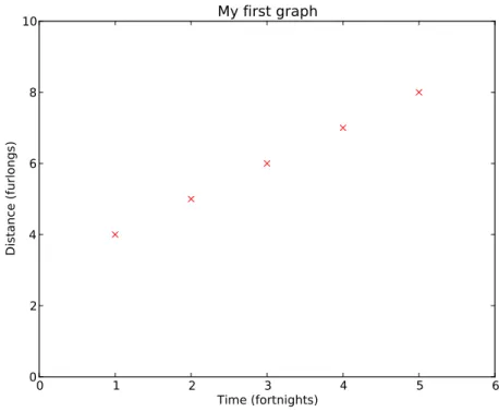
Next, we’ll tell Python to graph y versusx, using red×symbols:
In [3]: plot(x,y,’rx’)
Out[3]: [<matplotlib.lines.Line2D at (gibberish)>]
In addition to the nearly useless Out[] statement in your terminal window, you will note that a new window opens showing a graph with red×’s.
The graph is ugly, so let’s clean it up a bit. Enter the following commands at the iPython prompt, and see what they do to the graph window: (I’ve left out the In []: and Out[]: prompts.)
title(’My first graph’) xlabel(’Time (fortnights)’) ylabel(’Distance (furlongs)’) xlim(0, 6)
ylim(0, 10)
In the end, you should get something that looks like figure 0.
Let’s take a moment to talk about what’s we’ve done so far. For starters, x and y are variables. Variables in Python are essentially storage bins: x in this case is an address which points to a memory bin somewhere in the computer that contains anarray of 5 numbers. Python variables can point to bins containing just about anything: different types of numbers, lists, files on the hard drive, strings of text characters, true/false values, other bits of Python code,whatever! When any other line in the Python script refers to a variable, Python looks at the appropriate memory bin and pulls out those contents. When Python gets our second line
In [2]: y = x+3
It pulls out the x array, adds three to everything in that array, puts the resulting array in another memory bin, and makesy point to that new bin. The plot command plot(x,y, ’rx’ ) creates a new figure window if none exists, then makes a graph in that window. The first item in parenthesis is the x data, the second is the y data, and the third is a description of how the data should be represented on the graph, in this case red× symbols.
Here’s a more complex example to try. Entering these commands at the iPython prompt will give you a graph like figure 1:
0.0 Making graphs 3
0 1 2 3 4 5 6
Time (fortnights) 0
2 4 6 8 10
Distance (furlongs)
My first graph
Figure 0: A simple graph made interactively with iPython.
plot(time, height, ’m-^’)
plot(time, 0.3*sin(time*3), ’g-’)
legend([’damped’, ’constant amplitude’], loc=’upper right’) xlabel(’Time (s)’)
0 2 4 6 8 10 Time (s)
0.6 0.4 0.2 0.0 0.2 0.4 0.6 0.8 1.0
damped
constant amplitude
Figure 1: More complicated graphing example.
spot. Thelegend()command was given two parameters. The first parameter is alist3:
[ ’ damped ’ , ’ c o n s t a n t a m p l i t u d e ’ ]
Lists are indicated with square brackets, and the list elements are sepa-rated by commas. In this list, the two list elements are strings; strings are sequences of characters delimited (generally) by either single or double quotes. The second parameter in thelegend() call is a labeled option: these are often built in to functions where it’s desirable to build the functions with a default value but still have the option of changing that value if needed4.
3See section 1.3. 4
0.1 Libraries 5
0.1
Libraries
By itself, Python does not do plots. It doesn’t even do trig functions or square roots. But when you start iPython with the ‘-pylab’ option, you are telling it to load optionallibraries that expand the functionality of the Python language. The specific libraries loaded by ‘-pylab’ are mathematical and scientific in nature; but Python libraries are available to read web pages, create 3D animations, parse XML files, pilot autonomous aircraft, and just about anything else you can imagine. It’s easy to make libraries in Python, and you’ll learn how as you work your way through this class. But you will find that for many problems someone has already written a Python library that solves the problem, and the quickest and best way of solving the problem is to figure out how to use their library!
For plotting, the preferred Python library is “matplotlib”. That’s the library being used for the plots you’ve made in this chapter so far; but we’ve barely scratched the surface of what the matplotlib library is capable of doing. Take a look online at the “matplotlib gallery”: http://matplotlib. org/gallery.html. This should give you some idea of the capabilities of matplotlib. This page very useful: clicking on a plot that shows something similar to what you want to create gives example code showing how that graph was created!
Another extremely useful library for physicists is the ‘LINPACK’ linear algebra package. This package provides very fast routines for calculating
anything having to do with matrices: eigenvalues, eigenvectors, solutions of systems of linear equations, and so on. It’s loaded under the name ‘linalg’ when you use ipython−−pylab.
Example 0.1.1
In electronics, Kirchhoff’s laws are used to solve for the currents through components in circuit networks. Applying these laws gives us systems of linear equations, which can then be expressed as matrix equations, such as
−13 2 4
2 −11 6
4 6 −15
IA IB IC = 5 −10 5 (1)
This can be solved algebraically without too much difficulty, or one can simply solve it with LINPACK:
B = array([5,-10,5]) linalg.solve(A,B)
--> array([-0.28624535, 0.81040892, -0,08550186])
One can easily verify that the three values returned by linalg . solve () are the solutions for IA,IB, and IC.
LINPACK can also provide eigenvalues and eigenvectors of matrices as well, using linalg . eig (). It should be noted that the size of the matrix that LINPACK can handle is limited only by the memory available on your computer.
0.2
Reading data from files
It’s unlikely that you would be particularly excited by the prospect of man-ually typing in data from every experiment. The whole point of computers, after all, is tosave us effort! Python can read data from text files quite well. We’ll discuss this ability more in later in section 1.8, but for now here’s a quick and dirty way of reading data files for graphing.
We’ll start with a data file like that shown in table 1. This data file (which actually goes on for another three thousand lines) is from a lab ex-periment in another course at this university, and a copy has been provided5. Start iPython/pylab if it’s not open already, and then use theloadtxt()
func-Table 1: File microphones.txt
#Frequency Mic 1 Mic 2
10.000 0.654 0.192
11.000 0.127 0.032
12.000 0.120 0.030
13.000 0.146 0.031
14.000 0.155 0.033
15.000 0.175 0.036
. . .
tion to read columns of data directly into Python variables:
5
0.2 Reading data from files 7
frequency, mic1, mic2 = loadtxt(’microphones.txt’, unpack = True)
Theloadtxt() function takes one required argument: the file name. (You may need to adjust the file name (microphones.txt) to reflect the location of the actual file on your computer, or move the file to a more convenient location.) There are a number of optional arguments: one we’re using here is “unpack”, which tellsloadtxt()that the file contains columns of data that should be returnend in separate arrays. In this case, we’ve told Python to call those arrays ‘frequency’, ‘mic1’, and ‘mic2’. The loadtxt() function is very handy, and reasonably intelligent. By default, it will ignore any line that begins with ‘#’, as it assumes that such lines are comments; and it will assume the columns are separated by tabs. By giving it different optional arguments you can tell it to only read certain rows, or use commas as delimiters, etc. It will choke, though, if the number of items in each row is not identical, or if there are items that it can’t interpret as numbers.
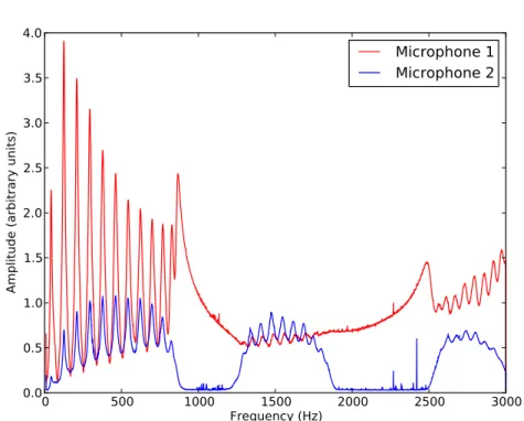
Now that we’ve loaded the data, we can plot it as before:
figure()
plot(frequency, mic1, ’r-’, frequency, mic2, ’b-’) xlabel(’Frequency (Hz)’)
ylabel(’Amplitude (arbitrary units)’) legend([’Microphone 1’, ’Microphone 2’])
0 500 1000 1500 2000 2500 3000 Frequency (Hz)
0.0 0.5 1.0 1.5 2.0 2.5 3.0 3.5 4.0
Amplitude (arbitrary units)
Microphone 1
Microphone 2
0.3 Problems 9
0.3
Problems
0-0 Graph both of the following functions on a single figure, with a usefully-sized scale.
(a)
x4e−2x (b)
x2e−xsin(x2)2
Make sure your figure has legend, range, title, axis labels, and so on.
0-1 The data shown in figure 2 is most usefully analyzed by looking at the
ratio of the two microphone signals. Plot this ratio, with frequency on thex axis. Be sure to clean up the graph with appropriate scales, axes labels, and a title.
0-2 The file Ba137.txt contains two columns. The first is counts from a Geiger counter, the second is time in seconds.
(a) Make a useful graph of this data.
(b) If this data follows an exponential curve, then plotting the natural log of the data (or plotting the raw data on a logrithmic scale) will result in a straight line. Determine whether this is the case, and explain your conclusion with —you guessed it— an appropriate graph.
0-3 The data in file Ba137.txt is actual data from a radioactive decay experiment; the first column is the number of decaysN, the second is the timet in seconds. We’d like to know the half-lifet1/2 of137Ba. It should follow the decay equation
N =Noe−λt
where λ= log 2t
1/2. Using the techniques you’ve learned in this chapter,
0-4 The normal modes and angular frequencies of those modes for a linear system of four coupled oscillators of massm, separated by springs of equal strength k, are given by the eigenvectors and eigenvalues of M, shown below.
M =
2 −1 0 0
−1 2 −1 0
0 −1 2 −1
0 0 −1 2
(The eigenvalues give the angular frequenciesω in units of
q
k
m.) Find
those angular frequencies.
0.3 Problems 11
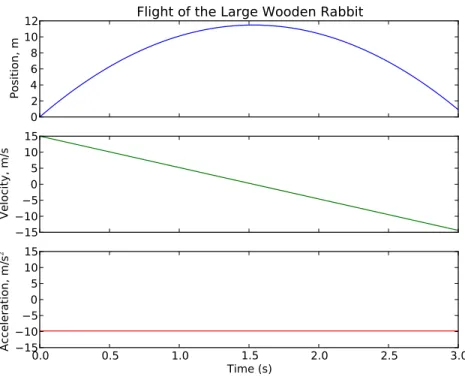
02 4 6 8 10 12
Position, m
Flight of the Large Wooden Rabbit
15 105 05 10 15
Velocity, m/s
0.0 0.5 1.0 1.5 2.0 2.5 3.0 Time (s)
15 105 05 10 15
Ac
ce
ler
at
ion
, m
/s
2
Chapter 1
Python Basics
1.0
The Python Interpreter
Python is a computer program which converts human-friendly commands into computer instructions. It is an interpreter. It’s written in another language; most often C++, which is more powerful and much faster, but also harder to use.1
There is a fundamental difference between interpreted languages (Python, for example) and compiled languages such as C++. In a compiled language, all the instructions are analyzed and converted to machine code by the com-piler before the program is run. Once this compilation process is finished, the program can run very fast. In an interpreted language, each command is analyzed and converted “on the fly”. This process makes interpreted lan-guages significantly slower; but the advantage to programming in interpreted languages is that they’re easier to tweak and debug because you don’t have to re-compile the program after every change.
Another benefit of an interpreted language is that one can experiment with simple Python commands by using the Python interpreter directly from the command line. In addition to the iPython method shown in the previous chapter, it’s possible to use the Python interpreter directly. From a terminal window (Macintosh or Linux) type python<enter>, or open a window in “Idle” (Windows). You will get the Python prompt: >>>. Try some simple mathematical expressions, such as 6*7<enter>. The Python interpreter takes each line of input you give it and attempts to make sense of it: if it can, it replies with what it got.
1There are versions of Python written in other languages, such as Java & C#. There
You can use Python as a very powerful calculator if you want. It can also store value in variables. Try this:
x = 4 y = 16 x*y x**y y/x x**y**x
That last one may take a moment or two: Python is actually calculating the value of 4(164), which is a rather huge number.
In addition to taking commands one line at a time, the Python inter-preter can take a file containing a list of commands, called aprogram. The rest of this book, and course, is about putting together programs so as to solve physics problems.
1.1
Comments
A program is a set of instructions that a computer can follow. As such, it has to be comprehensible by the computer, or it won’t run at all. The rest of this chapter is concerned with the specifics of making the program comprehensible to the computer, but it’s worthwhile to spend a little time here at the beginning to talk about making the program comprehensible to humans.
Python is pretty good in terms of comprehensibility. It’s a language that doesn’t require a lot of obscure punctuation or symbols that mean different things in different contexts. But there are still two very important things to keep in mind when you are writing any computer code:
(1) The next person to read the code will not know what you were thinking when you write the code.
(2) If you are the next person to read the code, rule #1 will still apply.
Because of this, it is absolutely critical to comment your code. Comments are bits of text in the program that the computer ignores. They are there solely for the benefit of any human readers.
Here’s an example Python program:
1.1 Comments 15
t e n P r i m e s . py
Here ’ s a s i m p l e Python program t o p r i n t t h e f i r s t 10 prime numbers . I t u s e s t h e f u n c t i o n I s P r i m e ( ) , w h i c h d o e s n ’ t e x i s t y e t , s o don ’ t t a k e t h e program t o o s e r i o u s l y u n t i l you w r i t e t h a t f u n c t i o n .
”””
# I n i t i a l i z e t h e prime c o u n t e r
c o u n t = 0
# ” number ” i s u s e d f o r t h e number we ’ r e t e s t i n g # S t a r t w i t h 2 , s i n c e i t ’ s t h e f i r s t prime .
number = 2
# Main l o o p t o t e s t e a c h number
while c o u n t < 1 0 :
i f I s P r i m e ( number ) : # The f u n c t i o n I s P r i m e ( ) s h o u l d r e t u r n # a t r u e / f a l s e v a l u e , d e p e n d i n g on # w h e t h e r number i s prime . T h i s # f u n c t i o n i s n o t b u i l t in , s o we ’ d # h a v e t o w r i t e i t e l s e w h e r e .
print number # The number i s prime , s o p r i n t i t .
c o u n t = c o u n t + 1 # Add one t o our c o u n t o f p r i m e s s o f a r .
number = number + 1 # Add one t o our number s o we can c h e c k # t h e n e x t i n t e g e r .
Anything that follows # is a comment. The computer ignores the com-ments, but they make the program easier for humans to read.
There is a second type of comment in that program also. Near the beginning there is a block of text delimited by three double-quotes: ”””. This is a multi-line string, which we’ll talk more about later. The string doesn’t do anything in this case, and isn’t used for anything by the rest of the program, so Python promptly forgets it and it serves the same purpose as a comment. This specific type of comment is used by thepydocprogram as documentation, so if you were to type the commandpydoc tenPrimes.py
the response would consist of that block of text. It is good practice to include such a comment at the beginning of each Python program. This comment should include a brief description of the program, instructions on how to use it, and the author & date.
#!/usr/bin/env python. This line is specific to Unix machines2. When the characters #! (called “hash-bang”) appear as the first two characters in a file, Unix systems take what follows as an indicator of what the file is supposed to be. In this case, the file is supposed to be used by whatever the program /usr/bin/envconsiders to be the pythonenvironment.
Compare the program above with the following functionally identical program:
c o u n t = 0 number = 2
while c o u n t < 1 0 :
i f I s P r i m e ( number ) :
print number
c o u n t = c o u n t + 1 number = number + 1
The second program might take less disk space but disk space is cheap and plentiful. Use the commented version.
1.2
Simple Input & Output
The raw input()command takes user keystrokes and assigns them, as a raw string of characters, to a variable. The input() command does nearly the same, the only difference being that it first tries to make numeric sense of the characters. Either command can give a prompt string, if desired.
Example 1.2.1
name = r a w i n p u t ( ” what i s your name? ” )
After the above line, the variable ’name’ will contain the char-acters you type, whether they be “King Arthur of Britain” or “3.141592”.
y = i n p u t ( ”What i s your q u e s t ? ” )
The value ofy, after you press enter, will be the computer’s best guess as to the numeric value of your entry. “3.141592” would result in y being approximately π. “To find the Holy Grail” would cause an error.
2
1.2 Simple Input & Output 17
In order to get your carefully calculated results out of the computer and onto the monitor, you need the print command. This command sends the value of its arguments to the screen.
Example 1.2.2 e = 2 . 7 1 8 2 8
print ” H e l l o , w o r l d ”
−→ Hello world
print e
−→ 2.71828
print ” E u l e r ’ s number i s a p p r o x i m a t e l y ” , e , ” . ”
−→ Euler’s number is approximately 2.71828 .
Note in example 1.2.2 that the comma can be used to concatenate out-puts. The comma can also be used to suppress the newline character that would otherwise come automatically at the end of the output. This use of the comma can allow you to make one print statement ending in a comma, then another print statement some lines further in the program, and have the output of both statements appear on one line of the screen.
It is also possible to specify the format of the output, using “string formatting”. The most common format indicators used for our purposes are given in table 1.1. To use these format indicators, include them in an output string and then add a percent sign and the desired value to insert at the end of the print statement.
Example 1.2.3 p i = 3 . 1 4 1 5 9 2
print ” Decimal : %d” % p i
−→3
print ” F l o a t i n g Point , two d e c i m a l p l a c e s : %0.2 f ” % p i
−→3.14
%xd Decimal (integer) value, with (optional) total widthx.
%x.yf
Floating Point value,x wide withydecimal places.Note that the output will contain more than x characters if necessary to show y decimal places plus the decimal point.
%x.ye Scientific notation, x wide withy decimal places.
%x.5g “General” notation: switches between floating point and sci-entific as appropriate.
%xs String of characters, with (optional) total width x.
+
A “+” character immediately after the % sign will force in-dication of the sign of the number, even if it is positive. Neg-ative numbers will be indicated, regardless.
Table 1.1: Common string formatting indicators
−→ 3.14e00
Note the two extra spaces at the front of the output in that final example. If we had given the format as “%2.2e”, the output would have been the same numerically, but without those two blank spaces at the beginning. The output format expands as necessary, but always takes upat least as much space as specified.
Should you need to include more than one formatted variable in your output, go right ahead: just put the variables, grouped with parenthesis, after the % sign. Put them in the right order, of course: the first value will go into the first string formatting code, the second into the second, and so on.
Example 1.2.4 p i = 3 . 1 4 1 5 9 2 e = 2 . 7 1 8 2 8 2 sum = p i + e
print ”The sum o f %0.3 f and %0.3 f i s %0.3 f . ” % ( p i , e , sum )
−→ The sum of 3.142 and 2.718 is 5.860.
1.3 Variables 19
C o m p l i c a t e d S t r i n g = ” S t u d e n t %s s c o r e d %d on t h e f i n a l exam , f o r a g r a d e o f %s . ” % ( name , FinalExamScore , F i n a l G r a d e )
1.3
Variables
It’s worth our time to spend a bit of time discussing how Python handles variables. When Python interprets a line such as x=5, it starts from the right hand side and works its way towards the left. So given the statement x=5, the Python interpreter takes the “5”, recognizes it as an integer, and stashes it in an integer-sized “box” in memory. It then takes the labelxand uses it as a pointer to that memory location. (See figure 1.0.)
x=5
y=x
x=3
y=3
5
5
5
3
3
3
5
x
x
x
y
y
y
x
Figure 1.0: Variable assignment statements, and how Python handles them. The boxes represent locations in the computer’s memory.
The statement y=x is analyzed the same way. Python starts from the right (x) and, recognizing x as a pointer to a memory location, makes y a pointer to the same memory location. At this point, bothxandyare point-ing to the same location in memory, and you could change the value of both
This right-to-left interpretation allows you to do some very useful —if mathematically improbable— things. For example, the command x = x+1 is perfectly legal in Python (as well as in nearly every other computer lan-guage.) If x = 3, as in the end of figure 1.0, Python would start from the right (x + 1) and calculate that to be “4”. It would then assign x to be a pointer to that “4”. It is also perfectly legal in Python to say w = x = y = z = ”Dead Parrot”. In this case, each of those variables would end up pointing at the exact same spot in memory, until they were used for something else.
Python also allows you to assign more than one variable at a time. The statementa,b = 3,5 works because Python analyzes the right half first and sees it as a pair of numbers, then assigns that pair to the pair of variables on the left.3 This can be used in some very handy ways.
Example 1.3.1
You want to swap two variable values.
x , y = y , x
Example 1.3.2
If you start witha=b= 1, what would be the result of repeated uses of this command?
a , b = b , a+b
Generally, a deep knowledge of how Python manages variables like this is not necessary. But there are occasions when changing a variable’s value changes the contents of that box in memory rather than changing the address pointed to by the variable. Keep this in mind when you’re dealing with matrices. It’s something to be aware of!
Variable Names
Variable names can contain letters, numbers, and the underscore character. They must start with a letter. Names are case sensitive, so “Time” is not the same as “time”.
3
1.3 Variables 21
It’s good practice when naming variables to choose your names so that the code is “self-commenting”. The variable names r and R are legal, and someone reading your computer code might guess that they refer to radii; but the names CylinderRadius and SphereRadius are much better. The extra time you spend typing those more descriptive variable names will be
more than made up by the time you save debugging your code!
Variable Types
There are many different types of variables in Python. The two broad divisions in these types are numeric types and sequence types. Numeric types hold single numbers, such as “42”, “3.1415”, and 2−3i. Sequence types hold multiple objects, which may be single numbers, or individual characters, or even collections of different types of things.
One of the strengths (and pitfalls) of Python is that it automatically converts between types as necessary, if possible.
Numeric Types
Integer The integer is the simplest numeric type in Python. Integers are perfect for counting items, or keeping track of how often you’ve done something.
The maximum integer is 231−1 = 2,147,483,647.
Integers don’t divide quite like you’d expect, though! In Python, 1/2 = 0, because 2 goes into 1 zero times.
Long Integer Integers larger than 2,147,483,647 are stored, automatically, as long integers. These are indicated by a trailing “L” when you print them, unless you use string formatting to remove it.
The maximum size of a long integer is limited only by the memory in your computer. Integers will automatically convert to long integers if necessary.
Float The “floating point” type is a number containing a decimal point. 2.718, 3.14159, and 6.626×10⁻³⁴are all floating point numbers. So is 3.0. Floats require more memory to store than do integers, and they are generally slower in calculations, but at least 1.0/2.0 = 0.5 as one would expect.
Python will convert the integer 2 to the float 2.0 and then do the math.There is a trade-off in speed for this convenience, though.
Complex Complex numbers are built-in in Python, which uses j ≡√−1. It is perfectly legal to sayx = 0.5 + 1.2jin Python, and it does complex arithmetic correctly.
Sequence Types
Sequence types in Python are collections of items which are referred to by one variable name. Individual items within the sequence are separated by commas, and referred to by an index in square brackets after the sequence name. This is easier to demonstrate than explain, so. . .
Example 1.3.3
Pythons = ( ” C l e e s e ” , ” P a l i n ” , ” I d l e ” , ”Chapman” , ” J o n e s ” , ” G i l l i a m ” )
print Pythons [ 2 ]
−→ Idle
Note that the index starts counting from zero:
print Pythons [ 0 ]
−→ Cleese
Negative numbers start counting from the end, backwards:
print Pythons [−1 ] , Pythons [−2 ]
−→ Gilliam Jones
One can also specify a “slice” of the sequence:
print Pythons [ 1 : 3 ]
−→ (’Palin’, ’Idle’)
Note that in that last example, what is printed is another (shorter) sequence. Note also that the range [1:3] tells Python to start with item 1 and goup to item 3. Item 3 is not included.
Now let’s examine some of the specific types of sequence in Python.
1.3 Variables 23
List Lists are indicated by square brackets: [ ]. Lists are pretty much the same as tuples, but they aremutable: individual items in a list may be changed. Lists can contain any other data type, including other lists.
String A string is a sequence of characters. Strings are delimited by either single or double quotes: “ ” or ‘ ’. Strings are immutable, like tuples. Unlike lists or tuples, strings can only include characters.
There are also some special characters in strings. To indicate a<tab> character, use “\t”. For a newline character, use “\n”.
The # character indicates a comment in Python, so if you put # in a string the rest of the string will be ignored by the Python interpreter. The way to get around this is to “escape” the character with “\”, such as “\#”. This causes Python to recognize that the # is meant as just a # character, rather than themeaning of #. Similarly,\” will allow you to put a double-quote inside a double-quoted string, and \’ will allow use of a single-quote inside a single-quoted string.
An alternate way of indicating strings is to bracket them in triple double-quotes. This allows you to have a string that spans multiple lines, including tabs and other special chacters. A triple double-quoted string within a Python program which is not assigned to a variable or otherwise used by Python will be taken to be documentation by the pydoc program.
Dictionary Dictionaries are indicated by curly brackets: { }. They are dif-ferent from the other built-in sequence types in Python in that instead of numeric indices they use “keys”, which are string labels. Dictionar-ies allow some very powerful coding, but we won’t be using them in this course so you’ll have to learn them elsewhere.
As mentioned in the description of lists above, a list can contain other lists. A list of lists sounds almost like a 2-dimensional array, or matrix. You can use them as such, and the way you would refer to elements in the matrix is to tack indices onto the end of the previous index.
Example 1.3.4
m a t r i x = [ [ 1 , 2 , 3 ] , [ 4 , 5 , 6 ] , [ 7 , 8 , 9 ] ]
m a t r i x [ 1 ] [ 0 ] = 0
(Remember that the indices start from zero!)
This is almost what we want for matrices in computational physics. Al-most. The [i][j] method of indexing is somewhat clumsy, for starters: it’d be nice to use [i,j] notation like we do in everything else. Another problem with using lists of lists for matrices is that addition doesn’t work like we’d expect. When lists or tuples or strings are added, Python just sticks them together end-to-end, which is mathematically useless.
Example 1.3.5
m a t r i x 1 = [ [ 1 , 2 ] , [ 3 , 4 ] ] m a t r i x 2 = [ [ 0 , 0 ] , [ 1 , 1 ] ]
print m a t r i x 1 + m a t r i x 2
−→ [ [1, 2], [3, 4] [0, 0], [1, 1] ]
The best way of doing matrices in Python is to use the SciPy or NumPy packages, which we will introduce later.
Sequence Tricks
If you are calculating a list of N numbers, it’s often handy to have the list exist first, and then fill it with numbers as you do the calculation. One easy way to create an empty list with the length needed is multiplication:
L o n g L i s t = [ ]∗N
After the above command,LongListwill be a list ofN blank elements, which you can refer to as you figure out what those elements should be.
Sometimes you may not know exactly how many list elements you need until you’ve done the calculation, though. Being able to add elements to the end of a list, thus making the list longer, would be ideal in this case; and Python provides for this with list .append(). Here’s an example:
Example 1.3.6
1.3 Variables 25
# S t a r t by c r e a t i n g t h e f i r s t l i s t e l e m e n t .
# Even an empty e l e m e n t w i l l do −− t h e r e j u s t must # b e s o m e t h i n g t o t e l l Python t h a t t h e v a r i a b l e # i s a l i s t r a t h e r t h a n s o m e t h i n g e l s e .
V a l u e s = [ ]
# Now do y o u r c a l c u l a t i o n s ,
NewValue = M u c h C a l c u l a t i o n ( YadaYadaYada )
# and e a c h t i m e you f i n d a n o t h e r v a l u e j u s t append # i t t o t h e l i s t :
V a l u e s . append ( NewValue )
# T h i s w i l l i n c r e a s e t h e l e n g t h o f V a l u e s [ ] by one , # and t h e new e l e m e n t a t t h e end o f V a l u e s [ ] w i l l # b e NewValue .
Another handy trick is sorting. If, for example, in the previous example you wanted to sort your list of values numerically after you’d calculated them all, this would do it:
V a l u e s . s o r t ( )
After that, the listValueswould contain the same information but in numeric order.
Generally speaking, the sort operation only works if all the elements of the list are the same type. Trying to sort a mix of numbers and strings and other sequences is a recipe for disaster, and Python will just give you an error and stop.
Sequences have many other useful built-in operations, more than can be covered here. Google is my preferred way of finding what they are: If there’s something you think you should be able to do with a sequence, Google “Python list (or string, or tuple) <action>”, whatever that action might be. This will usually come up with something! There are operations for finding substrings in strings, changing case in strings, removing non-printing characters, etc. . .
Ranges
integers beginning with Start (or zero if Start is omitted) and ending just beforeStop, incrementing by Stepalong the way.
Example 1.3.7
Create a list of 100 numbers for a graph axis.
a x i s = r a n g e ( 1 0 0 )
print a x i s
−→ [ 0, 1, 2, . . . 98, 99 ]
Create a list of even numbers from 6 up to 17.
Evens = r a n g e ( 6 , 1 7 , 2 )
List Comprehensions
The range() function only creates integers, and the spacing between the integers is always exactly the same. We often need something more flexible than that: what if we needed a list of squares of the first 100 integers, or a range that went up by 0.1 each step?
Python provides one very useful trick for doing just this thing: List Comprehensions. Again, this is most easily shown by example:
Example 1.3.8
Create a list of 100 evenly-spaced numbers for a graph axis which goes from a minimum of zero to a maximum of 2.
A x i s = [ 0 . 0 2 ∗ i f o r i in r a n g e ( 1 0 0 ) ]
Let’s look at that bit by bit. The square brackets indicate that the result is a list. The formuala (0.02 * i) is how it calculates each item in the list. The “for i in range(100)” tells Python to take each number in the list “range(100)”, call that number “i”, and apply the formula given.
List comprehensions work for any list, not just range(). So if you have a list of experimental measurements that were taken in inches, and you needed to convert them all to centimeters, then the line
1.4 Mathematical Operators 27
1.4
Mathematical Operators
In Python, the mathematical operators +− ∗() all work as one would expect on numbers and numeric variables. As mentioned previously, the + operator doesn’t do matrix addition on lists — it just strings them together instead. The * operator (multiplication) also does something unexpected on lists: if you multiply a list byn, the result will bencopies of the list, strung together. As long as you stick with numeric types, though, addition, subtraction, and multiplication do what you want.
Division (/) is slightly different. It works perfectly on floats, but on integers it does “third-grade math”: the result is always the integer portion of the actual answer.
Example 1.4.1
print 10/4
−→ 2
print 1/2
−→ 0
print 1 . / 2 .
−→ 0.5
That second case in example 1.4.1 is particularly bothersome: it causes more program bugs than you’d expect, so keep an eye out for it.
If you want “third-grade math” with floats, use the “floor division” op-erator, //.
Exponentiation in Python is done with the ∗∗operator, as in
S i x t e e n = 2∗∗4
The modulo operator (AKA “remainder”) is %, so 10%4 = 2 and 11%4 = 3.
Shortcut Operators
The statement x = x + y and other similar statements are so common in programming that many languages (including Python) allow shortcut oper-ators for these statements. The most common of these is+=, which means “Take what’s to the right and add to it whatever is on the left”. In other words, x += 1 is exactly equivalent to x = x + 1. Similarly,−=, ∗=, and /= do the same thing for subtraction, multiplication, and division.
These shortcut operators do not make your program run faster, and they do make the code harder for humans to read. Use them sparingly.
1.5
Lines in Python
Python is somewhat unique among programming languages in that it is whitespace-delimited. In other words, the Python interpreter actually cares about blank space before commands on a line.4 Lines are actually grouped by how much whitespace preceeds them, which forces one to write well-indented code!
When one speaks of “lines” of Python code, there are actually two types of line. A physical line is a line that takes up one line on the editor screen. Alogical line is more important — it’s what the Python interpreter regards as one line. Let’s look at some examples:
Example 1.5.1
print ” t h i s l i n e i s a p h y s i c a l l i n e and a l o g i c a l l i n e . ”
x = [ ” t h i s ” , ” l i n e ” , ” i s ” , ” both ” , ” a l s o ” ] x = [ ” t h i s ” , ” l i n e ” , ” i s ” , ” m u l t i p l e ” ,
” p h y s i c a l ” , ” l i n e s ” , ” but ” , ” i s ” , ” j u s t ” , ” one ” , ” l o g i c a l ” , ” l i n e ” ]
Indentation like this helps make programs clear and easier for humans to read. Python ignores extra whitespaceinsidea logical line, so it’s not a problem to put it there.
4
1.6 Control Structures 29
1.6
Control Structures
Control statements are statements that allow a program to do different things depending on what happens. “If you are hungry, eat lunch.” is a control statement of sorts. “While you are in Hawaii, enjoy the beach.” is another. Of course control statements in a computer language are a bit more specific than that, but they have the same basic structure. There is the statement itself: “if”. There is the “conditional”, which is a statement that evaluates to either true or false: “you are hungry”. And there is the action: “eat lunch”.
Conditionals
A conditional is anything that can be evaluated as either true or false. In Python, the following things are always false:
• The word False.
• 0, 0L, or 0.0
• ”” or ‘’ (an empty string)
• (), [], {} (The empty tuple, list, or dictionary)
Just about everything else is true.
• 1, 3.14, 42 (True, because they are numbers that aren’t zero)
• The word True.
• “False” (This is true, because it’s a string that is not empty. Python doesn’t look inside the string to see what it’s about!)
• “0”, for the same reason as “false”.
• [0, False , (), ””] (This is true, even though it’s a list of false things, because it is a non-empty list, and if a list is not empty then it is true.)
The comparisons are
< Less than
> Greater than
>= Greater than or equal to
== Equal to
! = Not equal to
Note that “=” is an assignment, and “==” is a conditional. FavoriteColor = ‘‘Blue’’ assigns the string “Blue” to the variable FavoriteColor, butFavoriteColor == ‘‘Blue’’ is a conditional that evaluates to either true or false depending on the con-tents of the variable FavoriteColor. Using = instead of == is one of the most common and hard-to-find bugs in Python programs!
There are also the boolean operatorsand,or, andnot.
Example 1.6.1
i f ( Animal == ‘ ‘ P a r r o t ’ ’ ) and (not I s A l i v e ( Animal ) ) : Complain ( )
The precedence ofand,or, andnotis the lowest of anything in Python, so the parentheses are not actually necessary. Those parentheses make the code more readable, though, and as such are highly recommended.
One final boolean is the in command, which is used to test whether an item is in a list.
Cast = ( ’ John ’ , ’ E r i c ’ , ’ Terry ’ , ’ Graham ’ , ’ Terry ’ , ’ M i c h a e l ’ )
i f Name in Cast :
print ’ Yes ’ , Name , ” i s a member o f Monty Python ’ s F l y i n g C i r c u s ”
If . . . Elif . . . Else
The most basic control statement in Python, or any other computer lan-guage, is the if statement. It allows you to tell the computer what to do if some condition is met. The syntax is as follows:
i f C o n d i t i o n a l : # The : i s n e e d e d a t t h e end o f t h i s l i n e .
DoThis ( ) # T h i s l i n e must b e i n d e n t e d .
AndThis ( ) # Any o t h e r l i n e s t h a t a r e p a r t o f t h e i f # s t a t e m e n t must a l s o b e i n d e n t e d t h e same # amount . ( comments a r e i g n o r e d , o f c o u r s e ! )
T h i s A l s o ( )
1.6 Control Structures 31
Note the indenting. In other computer languages, indentation like this makes the code easier to read; but in Pythonthe indentation is what defines the group of commands. The indentation is not optional.
The elif and else keywords extend the if statement even further. elif, short for “else if” adds another if that is tested only if the first if is false. elseis done if none of the previous elif statements, or the initial if, are true.
I f TestOne :
Do A ( ) # Do A ( ) i s done o n l y i f TestOne i s t r u e .
e l i f TestTwo : # TestTwo i s t e s t e d o n l y i f TestOne i s f a l s e .
Do B ( ) # Do B ( ) i s done i f TestOne i s f a l s e and # TestTwo i s t r u e .
e l i f T e s t T h r e e :
Do C ( ) # You can h a v e a s many e l i f ’ s a s you want , # o r none a t a l l . They ’ r e o p t i o n a l .
e l s e:
Do D ( ) # The ’ e l s e ’ i s what h a p p e n s i f n o t h i n g e l s e i s t r u e .
AlwaysDoThis ( ) # T h i s s t a t e m e n t i s b a c k a t t h e l e f t margin a g a i n . # That means i t ’ s a f t e r t h e end o f t h e w h o l e i f # c o n s t r u c t , and i t i s done r e g a r d l e s s .
While
Thewhilestatement is used to repeat a block of commands until a condition
is met.
while C o n d i t i o n : # The : i s r e q u i r e d , a g a i n .
DoThis ( ) # The b l o c k o f t h i n g s t h a t s h o u l d b e done
DoThat ( ) # i s i n d e n t e d , a s a l w a y s .
DoTheOther ( ) U p d a t e C o n d i t i o n ( )
# I f n o t h i n g h a p p e n s t o c h a n g e t h e c o n d i t i o n , # t h e w h i l e l o o p w i l l go f o r e v e r !
D o T h i s A f t e r w a r d s ( ) # T h i s s t a t e m e n t i s done a f t e r C o n d i t i o n # becomes f a l s e .
There are a few extra keywords that can be used with the while loop.
continue The continue keyword moves program execution to the top of the while block without finishing the portion of the block following
thecontinue statement.
break The breakkeyword moves execution of the loop directly to the line following thewhile block. It “breaks out” of the loop, in other words.
else An else command at the end of a while block is used to delineate a block of code that is done after the while block executes normally. The code in this block is not executed if the whileblock is exited via
a breakcommand.
Confusing enough for you? This is probably a good time for an example that uses these features.
Example 1.6.2
You need to write a program that tests whether a number is prime or not. The program should ask for the integer to test, then print a message giving either the first factor found or stating that the number is prime.
#! / u s r / b i n / env p y t h o n ”””
T h i s Python program d e t e r m i n e s w h e t h e r a number i s prime o r n o t . I t i s NOT t h e most e f f i c i e n t way o f d e t e r m i n i n g w h e t h e r a l a r g e i n t e g e r i s prime !
”””
# S t a r t by g e t t i n g t h e number t h a t m i g h t b e prime .
Number = i n p u t ( ”What i n t e g e r do you want t o c h e c k ? ” ) TestNumber = 2
# Main l o o p t o t e s t e a c h number
while TestNumber < Number :
i f Number % TestNumber == 0 :
# The r e m a i n d e r i s z e r o , s o TestNumber i s a f a c t o r # o f Number and Number i s n o t prime .
print Number , ” i s d i v i s i b l e by ” , TestNumber , ” . ”
# There i s no need t o t e s t f u r t h e r f a c t o r s .
break
e l s e:
# The r e m a i n d e r i s NOT z e r o , s o i n c r e m e n t
1.6 Control Structures 33
TestNumber += 1
e l s e:
# We g o t h e r e w i t h o u t f i n d i n g a f a c t o r , s o # Number i s prime .
print Number , ” i s prime . ”
For
Theforloop iterates over items in a sequence, repeating the loop block once per item. The most basic syntax is as follows:
f o r Item in S e q u e n c e : # The : i s r e q u i r e d
DoThis ( ) # The b l o c k o f commands t h a t s h o u l d
DoThat ( ) # b e done r e p e a t e d l y i s i n d e n t e d .
Each time through the loop, the value of Item will be the value of the next element in theSequence. There is nothing special about the namesItem and Sequence, they can be whatever variable names you want to use. In the case ofSequence, you can even use something that generates a sequence rather than a sequence, such asrange().
Example 1.6.3
You need a program to greet the cast of a humorous skit.
Cast = ( ’ John ’ , ’ E r i c ’ , ’ Terry ’ , ’ Graham ’ , ’ Terry ’ , ’ M i c h a e l ’ )
f o r Member in Cast :
print ’ H e l l o ’ , member # Each t i m e t h r o u g h t h e l o o p
# one c a s t member i s g r e e t e d .
print ’ Thank you f o r coming today ! ’ # T h i s l i n e i s o u t s i d e t h e l o o p
# s o i t i s done once , a f t e r # t h e l o o p .
The output of this program will be
Hello John Hello Eric Hello Terry Hello Graham Hello Terry Hello Michael
In numeric work, it’s more common to use the for command over a numeric range:
f o r j in r a n g e (N ) :
e t c ( )
Since therange()function returns a list, theforcommand is perfectly happy with that arrangement.
The for command also allows the same extras as while: continue goes straight to the next iteration of theforloop,break causes Python to aban-don the loop,elseat the end of the loop marks code that is doneonly if the forloop exits normally, and pass does nothing at all.
One caution about for loops: it’s quite possible to change the list that is controlling the loop during the loop! This is not recommended, as the results may be unpredictable.
1.7
Functions
A function is a bit of code that is given its own name so that it may be used repeatedly by various parts of a program. A function might be a bit of mathematical calculation, such as sin () or sqrt (). It might also be code to do something, such as draw a graph or save a list of numbers.
Functions are defined with the defcommand. The function name must start with a leter, and may contain letters, numbers, and the underscore character just like any other Python variable name. In parentheses after the function name should be a list of variables that should be passed to the function. Thedefline should end with a colon, and the indented block after thedefshould contain the function code.
Generally, a function shouldreturn some value, although this is not re-quired. For mathematical functions, the return value should be the result of the calculation. For functions that don’t calculate a mathematical value, the return should beTrue orFalse depending on whether the function managed to do what it was supposed to do or not.
Example 1.7.1
Write a function that calculates the factoral of a positive integer.
def f a c t o r a l ( n ) :
””” f a c t o r a l ( n )
1.7 Functions 35
most d i r e c t method i m a g i n a b l e . ”””
f = 1
f o r i in r a n g e ( 2 , n + 1 ) :
f = f ∗ i
return f
Once this definition has been made, any time you need to know the value of a factorial, you can just use factoral (x).
print ’ %10 s %10 s ’ % ( ’ n ’ , ’ n ! ’ )
f o r j in r a n g e ( 1 0 ) :
print ’ %10d %10d ’ % ( j , f a c t o r a l ( j ) )
Functions can also be used to break the code up into more understand-able chunks. Your morning ritual might look something like this, in Python code:
i f ( Time >= Morning ) : GetUp ( )
G e t D r e s s e d ( )
E a t B r e a k f a s t ( Spam , e g g s , Spam , Spam , Spam , Spam , bacon )
e l s e:
C o n t i n u e S l e e p i n g ( )
The functions GetDressed() and EatBreakfast() may entail quite a bit of code; but writing them as separate functions allows one to bury the details (socks first, then shoes) elsewhere in the program so as to make this code more readable. Writing the program as a set of functions also allows you to change the program easily, if for example you needed to eat breakfast before getting dressed.
The variables that are passed to the function exist for the duration of that function only. They may (or may not) have the same name(s) as other variables elsewhere in the program.
Example 1.7.2
def s q ( x ) :
# R e t u r n s t h e s q u a r e o f a number x
x = x∗x # Note t h a t s q ( ) c h a n g e s t h e l o c a l v a l u e o f x h e r e !
return x
# Here ’ s t h e main program :
print s q ( x ) # p r i n t s 9 ,
print x # p r i n t s 3 .
Note that the value ofxis changed within the functionsq(), but that change doesn’t “stick”. The reason for this is thatsq() does not receivex, but instead receives some value which it then calls x for the duration of the function. The x within the function is not the same as thex in the main program.
Functions can have default values built-in, which is often handy. This is done by putting the value directly into the definition line, like this:
def answer (A = 4 2 ) :
# Put y o u r f u n c t i o n h e r e # e t c .
# main program
answer ( 6 ) # For t h i s c a l l t o answer ( ) , A w i l l b e 6 .
answer ( ) # But t h i s time , A w i l l b e t h e d e f a u l t , 4 2 .
Global variables
If a Python function can’t find the value of some variable, it looks outside the function. This is handy: you can defineπ once at the beginning of the program and then use it inside any functions in the program. Values used throughout the program like this are called global variables.
If you re-define the value of a variable inside your function, though, then that new value is valid only within the function. To change the value of a global variable and make it stick outside the function, refer to that variable in the function as aglobal. The following example may help clarify this.
Example 1.7.3 a = 4
b = 5 c = 6
def f n ( a ) :
d = a # d i s a new l o c a l v a r i a b l e , and h a s t h e # v a l u e o f w h a t e v e r was p a s s e d t o f n ( ) .
1.7 Functions 37
# v a l u e o f ’ a ’ i s 5 now .
global c = 9 # I n s t e a d o f making a new l o c a l ’ c ’ , t h i s
# l i n e c h a n g e s t h e v a l u e o f t h e g l o b a l # v a r i a b l e ’ c ’ .
print a , b , c #−−> 4 5 6
f n ( b ) # The v a l u e o f d i n s i d e f n ( ) w i l l b e 5 . # The v a l u e o f a i n s i d e f n ( ) w i l l a l s o b e 5 .
print a , b , c #−−> 4 5 9
# The v a l u e s o u t s i d e f n ( ) d i d n ’ t change , # o t h e r t h a n c .
print d #−−>ERROR! d i s o n l y d e f i n e d i n s i d e f n ( ) .
Passing functions
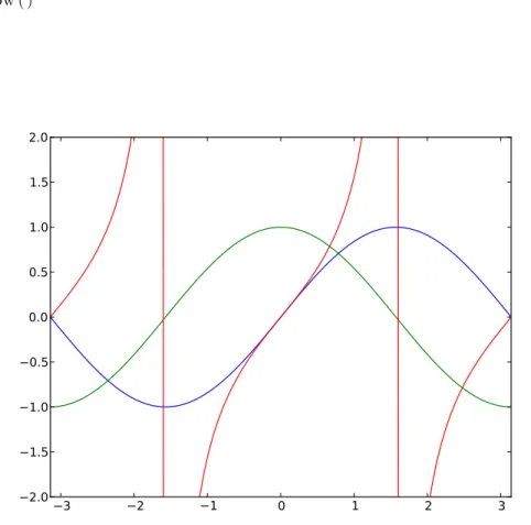
Python treats functions just like any other variable. This means that you can store functions in other variables or sequences, and even pass those functions to other functions. The following program is somewhat contrived, but it serves to give a good example of how this can be useful. The output is shown in figure 1.1.
#! / u s r / b i n / env p y t h o n ’ ’ ’ p a s s t r i g . py
D e m o n s t r a t e s Python ’ s a b i l i t y t o s t o r e f u n c t i o n s an v a r i a b l e s and p a s s t h o s e f u n c t i o n s t o o t h e r f u n c t i o n s .
’ ’ ’
from p y l a b import ∗
def p l o t t r i g ( f ) :
# t h i s f u n c t i o n t a k e s one argument , w h i c h must b e a f u n c t i o n # t o b e p l o t t e d on t h e r a n g e −p i . . p i .
x v a l u e s = l i n s p a c e (−p i , p i , 1 0 0 )
p l o t ( x v a l u e s , f ( x v a l u e s ) ) # y v a l u e s a r e computed d e p e n d i n g on f .
x l i m (−p i , p i ) # s e t x l i m i t s t o x r a n g e
y l i m (−2 , 2 ) # s e t t h e y l i m i t s s o t h a t t a n ( x ) d o e s n ’ t # r u i n t h e v e r t i c a l s c a l e .
t r i g f u n c t i o n s = ( s i n , c o s , t a n ) # t r i g f u n c t i o n s i s now a t u p l e t h a t h o l d s # t h e s e t h r e e f u n c t i o n s .
f o r f u n c t i o n in t r i g f u n c t i o n s :
# w i t h e a c h f u n c t i o n i n t h e l i s t .
print f u n c t i o n ( p i / 6 . 0 ) # r e t u r n s t h i s f u n c t i o n v a l u e .
p l o t t r i g ( f u n c t i o n ) # p a s s e s t h i s f u n c t i o n t o b e p l o t t e d .
show ( )
3 2 1 0 1 2 3
2.0 1.5 1.0 0.5 0.0 0.5 1.0 1.5 2.0
Figure 1.1: Output of function-passing program “passtrig.py”
1.8 Files 39
1.8
Files
More often than not in computational physics, the inputs and outputs of a project are large sets of data. Rather than re-enter these large data sets each time we run the program, we load and save the data in the form of text files.
When working with files, we start by “opening” the file. the open() function tells the computer operating system what file we will be working on, and what we want to do with the file. The function requires two parameters: the file name and the desired mode.
F i l e H a n d l e = open ( FileName , Mode )
FileName should be a string describing the location and name of the file, including any directory information if the file is not in the working directory for the Python program. The mode can be one of three things:
’r’ Read mode allows you to read the file. You can’t change it, only read it. ’w’ Write mode will create the file if it does not exist. If the file does exist, opening it in ’w’ mode will re-write it, destroying the current contents.
’a’ Append mode allows you to write onto the end of a previously-existing file without destroying what was there already.
Once the file is open for reading, we can read it by one of several methods. We can read the entire text file into one string:
s t r i n g = F i l e H a n d l e . r e a d ( )
The resulting string can be inconveniently huge, though, depending on the file! We could alternately read one line of the file at a time:
L i n e = F i l e H a n d l e . r e a d l i n e ( )
Each time you invoke this command, the variable Line will become a string containing the next line of the file indicated by FileHandle. We could also read all of the lines at once into a list:
L i n e s = F i l e H a n d l e . r e a d l i n e s ( )
After this command, Lines[0] will be a string containing the first line of the file, Lines[1] will contain the second line, and so on.
If you don’t close the file, it will close automatically when the program is done, but it’s still good practice to close it yourself.
Notice that all of these methods of reading a file result in strings of char-acters. This is to be expected, since the file itself is a string of characters on the drive. Python makes no effort to try figuring out what those charac-ters mean, so if you want to change the strings to numeric values you must convert them yourself by specifying what type of numbers you expect them to be. The float () and int () functions are the standard way of doing this. For example if the stringS = ’3.1415’, then x=float(S) takes that string and changes it to the appropriate floating-point value.
If you wish to write to a file, you must indicate so when you open the file.
F i l e H a n d l e = open ( FileName , ’w ’ )
After the file is open for writing, the write operation saves string information to the file:
F i l e H a n d l e . w r i t e ( s t r i n g )
Thewrite()operation is much more literal than theprintcommand: it sends to the file exactly the contents of the string. If the string does not have a newline character at the end, then there will be no newline character written to the file, so if you want to write a single line be sure to include ’\n’ as the last character in the string. The write() operation can use any of the string formatting techniques described earlier.
F i l e H a n d l e . w r i t e ( ” p i = %6.4 f\t e =%6.4 f\n” % ( p i , e ) ) When you are done writing to the file, it is very important to close the file.
F i l e H a n d l e . c l o s e ( )
Closing the file flushes the write buffer and ensures that all of the written matter is actually on the hard drive. The file will be closed automatically at the end of the program, but it’s better to close it yourself.
1.9
Expanding Python
1.9 Expanding Python 41
import math
import commands are generally placed at the beginning of the program,
although that’s just for convenience to the reader. Once the import com-mand has been run by the program, all of the functions in the “math” package are available as “math.(function-name)”.
import math
x = math . p i / 3 . 0
print x , math . s i n ( x ) , math . c o s ( x ) , math . t a n ( x )
There are many other functions and constants in the math package.5 It is often useful to just import individual elements of a package rather than the entire package, so that we could refer to “sin(x)” rather than math.sin(x).
from math import s i n
You can also import everything from a package, each with its own name:
from math import ∗
x = p i / 3 . 0
print x , s i n ( x ) , c o s ( x ) , t a n ( x )
There are numerous other packages that add useful functionality to Python. In this book we’ll be using the “scipy”, “pylab”, “matplotlib”, and “numpy” packages extensively. These will be discussed later, but one package that deserves mention here is the “sys” package, which allows access to some of the system underpinnings of a unix-based system. The part of the sys package we use most often is the variable sys.argv. When you invoke a Python program from the command line, it is possible to enter parameters directly at time of invocation.
$ add.py 35 7
In the case shown above, the variable sys.argv will be a list containing the program name and whatever came after on the line:
s y s . a r g v = [ ’ add . py ’ , ’ 35 ’ , ’ 7 ’ ]
So we can use this to enter values directly into a program.
Example 1.9.1
import s y s
x = f l o a t ( s y s . a r g v [ 1 ] ) # Note t h a t t h e i t e m s i n a r g v [ ]
y = f l o a t ( s y s . a r g v [ 2 ] ) # a r e s t r i n g s !
print ” %0.3 f + %0.3 f = %0.3 f ” % ( x , y , ( x+y ) )
5
If this program were saved as “add.py”, a user command of
add.py 35 7
would result in an output of
35.000 + 7.000 = 42.000
Note that the components of sys.argv are strings, so it’s neces-sary to convert them to floating-point numbers with the float () function so that they add as numbers.
You can also build your own packages. This is easier than you might imagine, since every Python program is a package already! Any Python program ending with a ’.py’ suffix on its filename (and they all should end with .py) can be imported by any other Python program. Just use from<filename>import <function(s)>.
Example 1.9.2
You’ve written a program called “area.py” that includes an inte-gration routine “integrate()”, and you’d like to use that routine in your next program.
from a r e a import i n t e g r a t e
It’s a good idea, as you work through the exercises in this course, to put any useful functions you may develop into a “tools.py” file. Then all of those functions are easily accessible from new programs with the command
from t o o l s import ∗
One thing to consider, though: any time you import a package, it over-writes anything with the same name. This can cause problems. The pylab package has trig functions, for example, that are capable of operating on entire arrays at once. The math package trig functions have much more basic capabilities. So if you use this code:
from p y l a b import ∗
from math import ∗
x = s i n ( [ 0 . 1 , 0 . 2 , 0 . 3 , 0 . 4 , 0 . 5 ] )
then the basic trig functions from math.py overwrite the pylab.py trig func-tions, and the sin () function will crash when you give it the array.
1.10 Where to go from Here 43
import p y l a b
import math
x = p y l a b . s i n ( [ 0 . 1 , 0 . 2 , 0 . 3 , 0 . 4 , 0 . 5 ] ) y = math . s i n ( p i / 2 )
There’s another thing to consider when dealing with Python packages:
any Python program can be imported as a package into any other Python program. A Python program can even import itself, which will cause nothing but trouble. Problems arise if you happen to name your program “math.py” and them import math, for example. Python will happily import the first “math.py” it finds, which will not be the one you expect and nothing will work right and the error messages you get will be completely unhelpful.
1.10
Where to go from Here
This chapter has barely scratched the surface of the Python language, but it hopefully gives you enough of a foundation in Python that you’ll be able to get started on solving some interesting physics problems.
There’s a lot more to learn. One excellent resource for learning more Python is the book Learning Python by Mark Lutz and David Ascher.[6] Another isComputational Physics by Mark Newman.[9] The official Python website is at http://www.python.org/, and it always has up-to-date doc-umentation about the latest version of Python. Google and other search engines are also excellent resources: there are numerous pages with helpful descriptions about how to do things in Python.
1.11
Problems
1-0 Use a list comprehension to create a list of squares of the numbers between 10 and 20, including the endpoints.
1-1 Write a Python program to print out the first N numbers in the Fi-bonacci sequence. The program should ask the user forN, and should require thatN be greater than 2.
1-2 For the model used in introductory physics courses, a projectile thrown vertically at some initial velocityvi has positiony(t) =yi+vit−12gt2,
where g = 9.8 m/s2. Write a Python program that creates two lists, one containing time data (50 data points over 5 seconds) and the other containing the corresponding vertical position data for this projectile. The program should ask the user for the initial height yi and initial
velocityvi, and should print a nicely-formatted table of the list values
after it has calculated them.
1-3 The energy levels for a quantum particle in a three-dimensional rect-angular box of dimensions{L1,L2, andL3}are given by
En1,n2,n3 =
¯ h2π2
2m
n21 L21 +
n22 L22 +
n23 L23
where the n’s are integers greater than or equal to one. Write a pro-gram that will calculate, and list in order of increasing energy, the values of the n’s for the 10 lowestdifferent energy levels, given a box for which L2 = 2L1 and L3= 4L1.
1-4 Write a function for
sinc(x)≡ sinx
x
Make sure that your function handles x= 0 correctly.
1-5 Write a function that calculates the value of thenthtriangular number. Triangular numbers are formed by adding a series of integers from 1 to n: i.e. 1 + 2 + 3 + 4 = 10 so 10 is a triangular number, and 15 is the next triangular number after 10.
1.11 Problems 45
1-7 Write a Python program to make an N ×N multiplication table and write this table to a file. Each row in the table should be a single line of the file, and the numbers in the row should be tab-delimited. Write the program so that it accepts two parameters when invoked: the size N of the multiplication table and the filename of the desired output file. In other words, the command to make a 5×5 table saved in file table5.txt would be
timestable.py 5 table5.txt
Chapter 2
Basic Numerical Tools
2.0
Numeric Solution
A problem commonly given in first-semester physics lab is to calculate the launch angle for a projectle launcher so that the projectile hits a desired target. This is an easy enough problem, if the launch point and the target are at the same elevation: you just take the range equation
R= v
2sin(2θ)
g
and solve forθ.
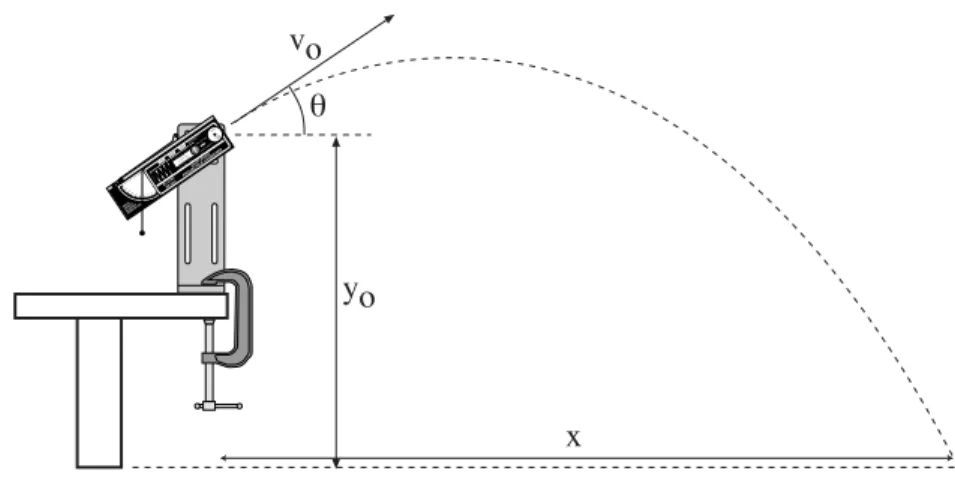
Complications arise, though, when the launcher is on the table and the target is on the floor. (See figure 2.0.)
To solve the problem in this case, we have to back up a bit and start with our basic kinematics equations. The horizontal distance traveled by the projectile in time tis
x=vxt (2.1)
wherevx is the horizontal component of the initial velocity,vx =vocosθ.
The timetat which the projectile hits the ground (and the target) is found by solving
0 =yo+viyt−
1 2gt
2 (2.2)
whereviy=vosinθand g= 9.8 m/s2. The solution to equation 2.2 is given
by the quadratic equation, so
t= 1
−g
−vosinθ±
q
v2
osin2θ+ 2yog