HungThesis Final

(1)

Effects of quantal and thermodynamical

fluctuations on superfluid pairing in nuclei

Doctoral Dissertation

by

Nguyen Quang Hung

Institute of Physics

10, Daotan street, Badinh district, Hanoi city, Vietnam

(2)

(3)

Acknowledgements

I would like to express my deep gratitude to my supervisor Dr. Nguyen Dinh Dang for

his guidance and encouragement during this research. He taught me not only physics

but also how to become an independent researcher. He always encourages me to develop

independent thoughts. He brought me the passion to research. My life really changed

after I met him.

I would like to thank Prof. Hoang Ngoc Long for his continuous support and great

advices to me since I was his Master’s student. He opened the door for me to theoretical

physics. I am greatly indebted to him.

I would like also to thank Prof. Pham Quoc Hung and Prof. Bach Thanh Cong of

Hanoi University of Science for their recommendations to the program of RIKEN Asia

Associate.

I am grateful to RIKEN Asia Program Associate for the financial support for my

research in RIKEN, and my life during my three-year stay in Japan between 2006 and

2009. This has been a very useful program for students from developing countries like

Vietnam to come to conduct research of high-quality international standard in RIKEN.

I am thankful to Dr. Y. Yano - director of RIKEN Nishina Center for Accelerator-Based

Science, Prof. T. Motobayashi - director of the Heavy-Ion Nuclear Physics Laboratory,

my RIKEN colleagues and friends for their continuous support, assistance, attention

to my research and to me. All the numerical calculations in the present dissertation

were carried out using the FORTRAN IMSL Library by Visual Numerics on the RIKEN

Super Combined Cluster (RSCC) system.

(4)

Global Relation Office), Ms. R. Kuwana (RIKEN Nishina Center) for their kind

assis-tances during my stay in RIKEN.

I am also thankful to Prof. S. Frauendorf (University of Notre Dame), Prof. V.

Zelevinsky (Michigan State University), Prof. B.A. Brown (Michigan State

Univer-sity), Prof. P. Danielewicz (Michigan State UniverUniver-sity), Prof. P. Schuck (Institute de

Physique Nucl´eaire - Orsay), Prof. L.G. Moretto (Lawrence Berkeley National

Lab-oratory), Dr. M. Sambataro (Istituto Nazionale di Fisica Nucleare), Dr. V. Kim Au

(Texas A&M University), Dr. A. Rios (Michigan State University), and Mr. I. Bentley

(University of Notre Dame) for fruitful discussions and various suggestions on a number

of issues included in this dissertation.

I am indebted to my parents, brother, sister, and my relatives in Vietnam for their

encouragement and confidence in me. Finally, I would like to thank my wife for her

(5)

Statement of authorship

I hereby certify that the present dissertation is my own research work. All the data

and results presented in this dissertation are true and correct. They are based on

the results and conclusions of four papers written in co-authorship with my thesis

supervisor Dr. N. Dinh Dang. Three of them have been published in international

peer-review journals, the fourth one is now under peer review. The anonymous referees

of these papers are qualified experts in the field. These results have also been reported

at 5 international meetings and 6 seminars in France, Germany, Italy, Japan, New

Zealand, and USA. This approbation process guarantees that these results have never

been published by anyone else in any other works or articles.

(6)

List of Tables

2.1 The energy difference ∆E ≡Eg.s.(G)−Eg.s.(0) at variousG(in MeV) as

predicted by the QRPA, SCQRPA, LNQRPA, LNSCQRPA, and exact

solutions for N = 10. . . 43

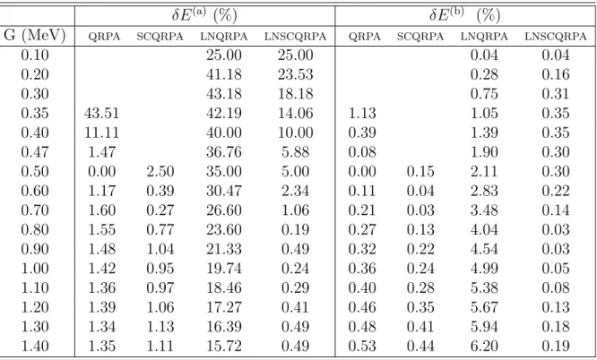
2.2 Relative errorsδE(a)_and_δE(b) _{from Eq. (2.54) at various}_G_{as predicted}

by the QRPA, SCQRPA, LNQRPA, and LNSCQRPA forN = 10. . . 44

2.3 BCS1 and LN1 pairing gaps (in MeV) at various values of G (in MeV)

(see text). . . 54

2.4 The ratio (δNj)2/hDji from Eqs. (2.19) and (2.20) corresponding to

the 5 lowest levels j = 1, . . . , 5, and the energies ω3 (in MeV) of the

first excited state described in the text for N = 10 at different values

of G (in MeV) within the LNSCQRPA. The energy ω3(a) is obtained

including the last term at the right-hand side of Eq. (2.19), while ω3(b)

(9)

List of Figures

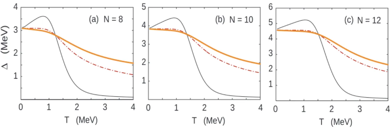
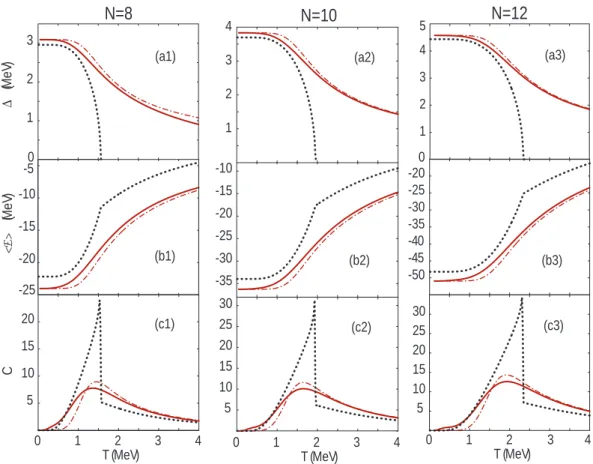
1.1 Pairing gaps ∆, total energies hEi, and heat capacities C, obtained for

N = 8, 10, and 12 (G= 0.9 MeV) within the FTBCS (dotted lines), CE

(dash-dotted lines), and GCE (solid lines) vs temperatureT. . . 20

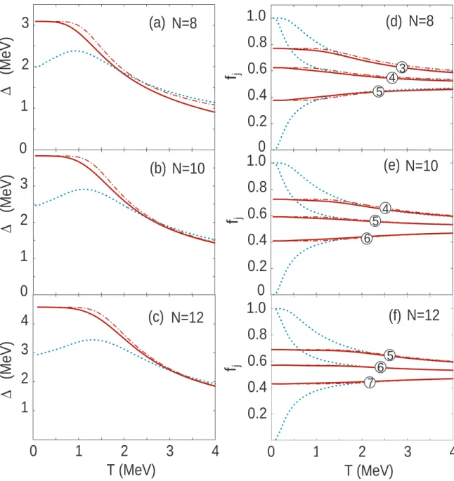
1.2 Pairing gaps (1.42) and single-particle occupation numbersfj forN = 8,

10, and 12, obtained within the mean field (dotted lines) as functions of

T, in comparison with the GCE gaps (solid lines), and CE (dash-dotted

lines) ones. . . 22

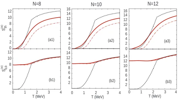
1.3 Thermodynamic entropyS_th(α), and quasiparticle (single-particle) entropy

Sq.p.(α), obtained forN = 8, 10, and 12 (G= 0.9 MeV) vsT. The notations

forα = FTBCS, CE, and GCE are the same as in Fig. 1.1. . . 23

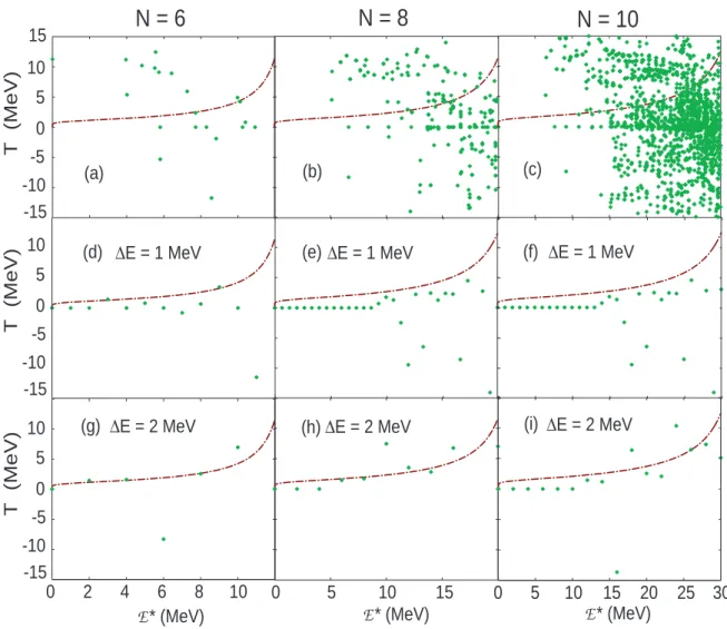
1.4 Temperature extracted from Eq. (1.37) within the MCE (dots) vs

exci-tation energy E∗ _{in comparison with the CE results (dash-dotted line)}

for N = 8, 10, and 12. The results in the top panels, (a) – (c), are

obtained by using Eq. (1.31), whereas those in the middle panels, (d) –

(f), and bottom ones, (g) – (i), are calculated by using Eq. (1.37) with

two different values of the energy interval ∆E in the statistical weight

Ω in Eq. (1.36). . . 25

1.5 Temperatures [(a) – (c)], entropies [(d) – (f)], and pairing gaps [(g) – (i)]

within the MCE as functions of excitation energy E∗ _for _N _{= 8 (}_G ₌

0.9 MeV) obtained by using the Gaussian, Lorentz, and Breit-Wigner

distributions from Eq. (1.38) for the level density at different values of

(10)

1.6 Pairing gaps extracted from the odd-even mass differences as functions

of T for N = 8, 10, and 12. The thin solid and thick solid lines denote

the gaps ∆(β, N) from Eq. (1.43), and the modified gaps ∆(e β, N) from

Eq. (1.45), respectively. The dash-dotted lines are the same canonical

gaps ∆C as in Figs. 1.1 and 1.2. . . 27

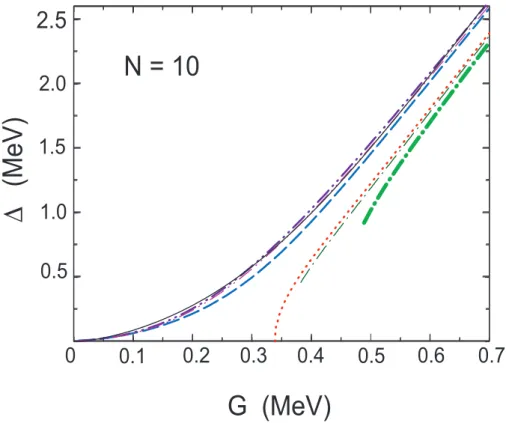
2.1 Pairing gaps ∆ as functions of G for N=10. The dotted, thin and

thick dash-dotted denote the BCS, RBCS, and BCS1 results,

respec-tively while the dashed, thick and thin dash-double-dotted lines

repre-sent the LN1, LN and RLN results, respectively.. The thin solid line

depicts the exact gap (see the text). . . 41

2.2 Ground state energies as functions of G for N = 10. The exact result

is represented by the thin solid line in both panels (a) and (b). In

panel (a), the dotted line denotes the BCS result, the thin dashed line

stands for the LN result, the dash-dotted line shows thepp RPA result

atG≤GBCS

c , and the QRPA one at G > GBCSc , while the

dash–double-dotted line depicts the LNQRPA result. Predictions by self-consistent

approaches are plotted in panel (b), where the thick dashed line denotes

the SCRPA result, while the SCQRPA and LNSCQRPA are shown by

the thick solid and thin double-dash–dotted lines, respectively. . . 42

2.3 Chemical potentials λand λ± _{as functions of}_G _for_N _{= 10 as predicted}

by the exact solutions, RPA, QRPA, SCRPA, SCQRPA, and

LNSC-QRPA. Notations are as in Fig. 2.2. . . 46

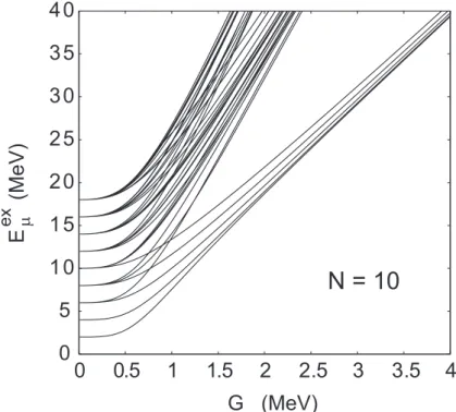
2.4 Exact energies Eex

µ ≡ Eµex(N)− E0ex(N) obtained within the Richardson

model for excited statesµrelative to the exact ground-state levelEex 0 as

(11)

2.5 The energies of the first excited state as functions of G at N=10. The

results refer to the exact solution, Eex

1 (solid line), the QRPA

solu-tion, ωQRPA₂ (dash-dotted line), the SCQRPA solution, ω₂SCQRPA (thick solid line), the LNQRPA solutions,ω₂LNQRPA(thin dash – double-dotted line) and ω₃LNQRPA (thick dash – double-dotted line), as well as the LNSCQRPA solutions,ω₂LNSCQRPA (thin double-dash – dotted line) and

ω₃LNSCQRPA (thick double-dash – dotted line). . . 48 2.6 The energies of the first excited state in different schemes as functions of

Gfor N = 10. The thin and thick dash – double-dotted lines denote the

second and third LNQRPA solutions, while the thin and thick dotted

lines stand for the absolute values of the corresponding solutions within

the LNQRPA1 scheme. . . 50

2.7 Energies of ground state (left panels) (notations as in Fig. 2.2) and first

excited state (right panels) (notations as in Fig. 2.5) for several values

of N indicated on the panels as functions of G. . . 52

2.8 Energy ∆ω(SC)RPA_{(2.57) obtained within the}_pp_{RPA (dash-dotted line)}

and SCRPA (thick solid line) as a function of G for several values of

N in comparison with the energy ωLNQRPA₃ (dash – double-dotted line),

ω₃LNSCQRPA (double-dash – dotted line), and the exact energy Eex 1 (thin

solid line), which are the same as those in Fig. 2.7 (d) – (f) forN = 4,

(12)

3.1 Diagrams summarized within the FTBCS1+SCQRPA. An arrow thin

line denotes the quasiparticle propagation, whereas a wavy line

repre-sents an SCQRPA phonon. The free quasiparticle Green function G0 j is

shown as the graph (a), whereas the loops in (b) and (c) stand for the

first and second summations at the right-hand side of Eq. (3.29),

respec-tively. An open circle in (b) denotes the vertex∼V_jµp1−nj +νµ, while

a box in (c) stands for ∼ V_jµ√nj +νµ. An SCQRPA phonon is

repre-sented in (d) as a sum of forward- and backward-going time conjugated

quasiparticles pairs. . . 65

3.2 (Level-weighted pairing gaps ∆ obtained within the FTBCS1 as

func-tions of temperature T at various values of pairing parameter G (in

MeV) indicated by the figures near the lines for several values of particle

number N. Open circles on the axes of abscissas in panels (a) and (b)

mark the valuesT1 of temperature, where the FTBCS1 gap turns finite

at low G. Full circles denote temperature Tec, where the gap vanishes,

and T2, where it reappears. . . 69

3.3 Level-dependent pairing gap ∆j (3.2) and level-weighted pairing gap ∆

(3.36) obtained within the FTBCS1 as functions of temperature T for

N = 20 andG= 0.44 MeV. Thick solid lines represent the level-weighted

gaps ∆. Thin solid lines denote the level-dependent gaps ∆j

correspond-ing to thej-th orbitals, whose level numbers j are marked at the lines.

Dashed and dotted lines stand for the level-independent part (quantal

component), ∆, and the level-dependent one (thermal component),δ∆j,

(13)

3.4 Level-weighted pairing gaps (a, d), total energies (b, e), and heat

capac-ities (c, f) as functions of temperatureT, obtained forN = 10 [(a) – (c)],

andN = 50 [(d) – (f)]. The dotted, thin solid, thick solid lines show the

FTBCS, FTBCS1, and FTBCS1+SCQRPA results, respectively. The

predictions by the FTLN1 and FTLN1+SCQRPA are presented by the

thin and thick dashed lines, respectively. The thin and thick dash-dotted

lines in (a) – (c) denote results of the GCE and CE ensembles,

respec-tively. The calculations of the mass operator and quasiparticle damping

within the SCQRPA were performed usingε= 0.05 MeV. . . 74

3.5 Level-weighted pairing gaps, total energies, and heat capacities for 10

neutrons in the 1f7/22p3/22p1/21f5/2 shell of 56Fe and all neutron bound

states of120_{Sn as functions of} _T ₍_ε_{= 0.1 MeV). Notations are as in Fig.}

3.4. In (b) and (c), the predictions by the finite-temperature quantum

Monte Carlo method [59] are shown as boxes and crosses with error bars

connected by dash-dotted lines. . . 76

3.6 Quasiparticle occupation numbers for N = 10 with G = 0.4 MeV (a,

b) and 120_{Sn with} _G _{= 0.137 MeV (c) as functions of} _T_{. In (a) and}

(b) the solid lines are predictions within FTBCS1+SCQRPA for the

levels numerated by the numbers in the circles starting from the lowest

ones. The dashed lines, numerated by the italic numbers, show the

corresponding results obtained within the FTBCS1. In (c) predictions

for the neutron orbitals of the (50 - 82) shell in 120_{Sn, obtained within}

the FTBCS1 and FTBCS1+SCQRPA, are shown as the dashed and solid

lines, respectively. . . 77

3.7 Level-weighted gaps for N = 10 with G = 0.4 MeV as predicted by

the WT (dashed), HP (dash-dotted), and QBA (thin dotted)

approxi-mations in comparison with the FTBCS (thick dotted), FTBCS1 (thin

(14)

4.1 Level-weighted pairing gaps ¯∆ as functions of T at various M [(a), (d)],

and as functions ofM [(b), (e)] andγ [(c), (f)] at several T for N = 10,

G= 0.5 MeV obtained within the FTBCS (left) and FTBCS1 (right). 91

4.2 Same as Fig. 4.1 but for neutrons in 20_{O using} _G_{= 1.04 MeV.} _{. . . .} ₉₄

4.3 Same as Fig. 4.1 but for neutrons in 44_{Ca using} _G_{= 0.48 MeV. . . . .} ₉₇

4.4 Level-weighted pairing gaps as functions of T at various M obtained

within the FTBCS (left) and FTBCS1 (right) for neutrons [(a), (c)],

and protons [(b), (d)] in 22_{Ne using} _G

n= 1.0 MeV and Gp = 1.32 MeV. 98

4.5 Moment of inertia as a function of the square γ2 _{of angular velocity} _γ

obtained within the FTBCS (left) and FTBCS1 (right) at various T for

N = 10 [(a), e)], neutrons in 20_{O [(b), (f)] and} 44_{Ca [(c), (g)], and the}

whole22_{Ne nucleus (including both proton and neutron gaps) [(d), (h)].} ₉₉

4.6 Level-weighted pairing gaps ¯∆ for N = 10 with G= 0.5 MeV [ε = 0.1

MeV in Eqs. (4.26) and (4.27)]. (a1) – (c1): ¯∆ vs temperature T at

different angular momentaM. (a2) – (c3): Results obtained at different

values of T, namely, (a2) – (c2): ¯∆ vs M; (a3) – (c3): ¯∆ vs angular

velocity γ. The dotted, thin solid, thick solid, thin dash-dotted, thick

dash-dotted lines are results obtained within the FTBCS, FTBCS1,

FT-BCS1+SCQRPA, FTLN1, FTLN1+SCQRPA, respectively. The solid

lines with circles and boxes in (a1) and (a3) correspond to two

defini-tions ∆(1)c and ∆(2)c of the canonical gaps at T = 0, respectively (See

Sec. 4.4.6). In (a2) the dashed lines connecting the discrete values of

the corresponding canonical gaps atT = 0 are drawn to guide the eye. 101

4.7 Moment of inertia J as function of the squareγ2 _{of angular velocity at}

various T for N = 10 with G= 0.5 MeV (ε = 0.1 MeV). Notations are

(15)

4.8 Level-weighted pairing gaps ¯∆, total energies E, and heat capacities C

as functions of temperatureT for three values of angular momentumM

obtained within the FTBCS (dotted lines), FTBCS1 (thin solid lines)

and FTBCS1 + SCQRPA (thick solid lines) for neutrons in 20_{O with}

G= 1.04 MeV (ε= 0.1 MeV). . . 104

4.9 Same as in Fig. 4.8 but for neutrons in 44_{Ca with} _G _{= 0.48 MeV (}_ε ₌

1 MeV). . . 105

4.10 (a) Canonical moment of inertia vs γ2_{; (b): Absolute values} _|hEi C −

Em.f.| (solid line) and |Eunc.| (dotted line) vs γ; (c): [∆(1)C ]2 vs γ for the

(16)

Introduction

Many experiments on heavy-ion fusion reaction had been carried out in the last two

decades (See Ref. [37] for a detail account). In these experiments compound nuclei

at highly excitation energies were created. The time required for these compound

nuclei to reach thermal equilibrium is around 10−23 _{seconds, which is much shorter}

than the typical time of ∼ 10−15 _{seconds, after which they start to decay. Therefore}

one can apply statistical thermodynamics to these highly-excited nuclei, and assign for

them a temperature T, which is extracted from their total or excitation energies after

subtracting the contribution due to angular momentum. This is why such systems

can be referred to as nuclei at finite temperature or hot nuclei. The typical range of

temperature for a self-sustained thermally equilibrated nucleus is below the neutron

binding energy, which is T < 6 – 8 MeV for heavy nuclei.

Phase transitions are common features of infinite systems in thermodynamics. At

the phase-transition point, called critical point, physical properties of the system

un-dergo an abrupt change. Phase transitions like the one from the superfluid

(supercon-ducting) state to the normal state are experimentally found in metal superconductors,

ultracold gases, liquid helium, etc. They are described very well by the many-body

mean-field theories, such as the Bardeen-Cooper-Schrieffer (BCS) [3] theory for the

superfluid-normal (SN) phase transition. Fluctuations play no role in these systems

as their effects are either zero in infinite systems or negligible for very large systems.

However, in small finite systems such as atomic nuclei or ultrasmall superconducting

(17)

finiteness of these systems. Therefore, in order to be reliable, the well-known

many-body theories such as the BCS theory or random-phase approximation (RPA) [58],

which is a theory to describe small-amplitude vibrations around the mean field, need

to be corrected to take into account the effects of quantal and thermal fluctuations.

Zero temperature

At zero temperature, one of standard methods to treat the quantal correlations beyond

the mean field is the well-known random-phase approximation (RPA). Extensively

employed in nuclear systems, the RPA includes correlations in the ground state, and

provides a simple theory of excited states of the nucleus. However, the RPA breaks

down at a certain value Gc of interaction parameter G, where it yields imaginary

solutions. The reason is that the RPA equations, linear with respect to the X and

Y amplitudes of the RPA excitation operator, are derived based on the quasi-boson

approximation (QBA). The latter neglects the Pauli principle between fermion pairs,

and its validity is getting poor with increasing the interaction parameter G. The

collapse of the RPA at the critical value Gc of G invalidates the use of the QBA. The

RPA therefore needs to be extended to correct this deficiency, at least for finite systems

such as nuclei.

One of methods to restore the Pauli principle is to renormalize the conventional

RPA to include the non-zero values of the commutator between the fermion-pair

oper-ators in the correlated ground state. These so-called ground-state correlations beyond

RPA cause the quantal fluctuations, whose effects are neglected within the QBA. The

interaction in this way is renormalized and the collapse of RPA is avoided. The

result-ing theory is called the renormalized RPA (RRPA) [36, 62, 9]. However, the test of

the RRPA carried out within several exactly solvable models showed that the RRPA

results are still far from the exact solutions of the models [9, 27, 38].

Recently, a significant development in improving the RPA has been carried out

(18)

of renormalizing the particle-particle (pp) RPA, the SCRPA made a step forward by

including the screening factors, which are the expectation values of the products of two

pairing operators in the correlated ground state. The SCRPA has been applied to the

exactly solvable multi-level pairing model, where the energies of the ground state and

first excited state in the system withN+2 particles relative to the energy of the

ground-state level in theN-particle system are calculated and compared with the exact results.

It has been found that the agreement with the exact solutions is good only in the weak

coupling region, where the pairing-interaction parameter Gis smaller than the critical

valuesGc. In the strong coupling region (G >> Gc), the agreement between the SCRPA

and exact results becomes poor [27, 38]. In this region a quasiparticle representation

should be used in place of theppone, as has been pointed out in Ref. [21]. As a matter

of fact, an extended version of the SCRPA in the superfluid region has been proposed

and is called the self-consistent quasiparticle RPA (SCQRPA), which was applied for

the first time to the seniority model in Ref. [28] and a two-level pairing model in Ref.

[55]. The derivations of the SCQRPA equations were based on the

Bardeen-Cooper-Schrieffer (BCS) [3] equations and self-consistently coupled to the quasiparitcle RPA

(QRPA). However, the SCQRPA also collapses at G = Gc. It is therefore highly

desirable to develop a SCQRPA that works at all values ofGand also in more realistic

cases, e.g., multilevel models. One of the aim of present study is to construct such

an approach. Obviously, the collapse of the SCQRPA at G = Gc, which is the same

as that of the non-trivial solution for the pairing gap within the BCS theory, can be

avoided by performing the particle-number projection (PNP). The latter removes the

quantal fluctuations caused by particle-number violation inherent in the BCS wave

functions. The Lipkin-Nogami method [47, 54], which is an approximated PNP before

variation, will be used in such extension of the SCQRPA in the present study because

of its simplicity. This approach shall be applied to a multi-level pairing model, the

so-called Richardson model [57], which is an exactly solvable model extensively employed

(19)

Finite temperature

At finite temperature, fluctuations strongly affect thermal pairing correlations in

nu-clear systems, which has been extensively studied within the BCS theory at finite

temperatureT (FTBCS theory) [3]. The FTBCS theory predicts a destruction of

pair-ing correlation at a critical temperatureTc '0.568∆(0) [∆(0) is the pairing gap at zero

temperature], resulting in a sharp transition from the superfluid phase to normal one

(the SN phase transition) [30, 45] in good agreement with the experimental findings

in macroscopic systems such as metallic superconductors. However, the BCS theory is

valid only when the assumption on the quasiparticle mean field is good, i.e. when the

difference between the pair operator P_jm† ≡a†_jma_j†₋_m and its expectation valuehP_jm† iis small so that the quadratic term (P_jm† − hP_jm† i)2 _{is negligible, where}_a†

jm is the operator

that creates a particle with angular momentum j and spin projection m. For small

systems such as atomic nuclei or for underdoped cuprates, where the coherence lengths

(the Cooper-pair sizes) are very short, the fluctuations (P_jm† − hP_jm† i)2 _{are no longer}

small, which invalidate the quasiparticle mean-field assumption, and break down the

BCS theory. As the result, the gap evolves continuously across Tc, and persists well

above Tc [26, 42].

The effects of thermal fluctuations on the pairing properties of nuclei have been

the subject of numerous theoretical studies in the last three decades. In the seventies,

by applying the macroscopic Landau theory of phase transitions to a uniform model,

Moretto has shown that thermal fluctuations smooth out the sharp SN phase

transi-tion in finite systems [49]. In the eighties, this approach was incorporated by Goodman

into the Hartree-Fock-Bogoliubov (HFB) theory at finite temperature [32] to account

for the effect of thermal fluctuations [33]. Theoretical studies within the static-path

approximation (SPA) carried out in the nineties also came to the non-vanishing pairing

correlations at finite temperature [60], which are qualitatively similar to the predictions

(20)

calculations [73, 24] also show that pairing does not abruptly vanish atTc, but still

sur-vives atT > Tc. The recent microscopic approach to thermal pairing, called

modified-HFB (Mmodified-HFB) theory [18], includes the quasiparticle-number fluctuation (QNF) in the

modified single-particle density matrix and particle-pairing tensor. Its limit of constant

pairing interactionGis the modified BCS (MBCS) theory [22, 19, 12, 13]. The MBCS

theory predicts a pairing gap, which does not collapse at Tc, but monotonously

de-creases with increasingT, in qualitative agreement with the predictions by the Landau

theory of phase transitions and SPA. This feature also agrees with the results obtained

by averaging the exact eigenvalues of the pairing problem over the canonical ensemble

(CE) with a temperature-dependent partition function [12]. The recent extraction of

pairing gap from the experimental level densities [42] confirms that the pairing gap

does not vanish atTc but decreases asT increases, in line with the predictions by these

approaches.

The above mentioned approaches are based on the independent quasiparticles,

whose occupation numbers follow the Fermi-Dirac distribution of free fermions.

Dy-namic effects such as those due to coupling to small-amplitude vibrations within the

RPA are ignored. These effects have recently been explored by extending the SCRPA

to finite temperature using the double-time Green’s function method [21]. However,

the finite-temperature SCRPA also fails in the region of strong pairing, where it should

be replaced by the quasiparticle representation. Therefore, it is highly desirable to

develop a self-consistent quasiparticle RPA (SCQRPA) at finite temperature, which is

workable at any value of pairing interaction parameter G.

The thermodynamic averages of the exact solutions of the pairing Hamiltonian are

usually carried out within CE assuming that nucleus is a system with a fixed number of

particles, and the results are compared with those obtained within different theoretical

approximations at finite temperature. However, the latter are always derived within the

grand canonical ensemble (GCE), where both energy and particle number are allowed

(21)

should be extracted from the microcanonical ensemble (MCE) of thermally isolated

nuclei is also quite often debated and studied in detail [73]. In thermodynamics limit

(i.e. when the system’s particle number N and volume V approach infinity, but N/V

is finite), fluctuations of energy and particle number are zero, therefore three types

of ensembles offer the same average values for thermodynamic quantities.

Thermo-dynamics limit works quite well in large systems as well where these fluctuations are

negligible. The discrepancies between the predictions by three types of ensembles arise

when thermodynamics is applied to small systems such as atomic nuclei or

nanometer-size clusters. These systems have a fixed and not very large number of particles, their

single-particle energy spectra are discrete with the level spacing comparable to the

pairing gap. Under this circumstance, the justification of using the GCE for these

sys-tems becomes questionable. These results suggest that a thorough comparison of the

predictions offered by the exact pairing solutions averaged within three principal

ther-modynamic ensembles, and those given by the recent microscopic approaches, which

include fluctuations around the thermal pairing mean field in nuclei, might be timely

and useful. This question is not new, but the answers to it have been so far only partial.

Already in the sixties Kubo [43] drew attention to the thermodynamic effects in

very small metal particles. Later, Denton et al. [25] used Kubo’s assumption to study

the difference between the predictions offered by the GCE and CE for the heat

ca-pacity and spin susceptibility within a spinless equidistant level model for electrons.

Very recently, the predictions for thermodynamic quantities such as total energy, heat

capacity, entropy, and microcanonical temperature within three principal ensembles

were studied and compared in Ref. [68] by using the exact solutions of an equidistant

multilevel model with constant pairing interaction parameter. However, no results for

the pairing gaps as functions of temperature were reported. It would be, therefore,

in-teresting to make a systematic comparison of predictions for nuclear pairing properties

obtained by averaging the exact solutions in three principle ensembles as well as those

(22)

Finite angular momentum

Fluctuations affect not only the nuclear systems at zero and finite temperature, but

also the rotating nuclei. The rotational phase of nucleus as a whole, such as that in

spherical nuclei, is known to affect nuclear level densities. The relationship between this

noncollective rotation and pairing correlations has been the subjects of many theoretical

studies. The effect of thermal pairing on the angular momentum at finite temperature

was first examined by Kammuri in Ref. [40], who included in the FTBCS equations the

effect caused by the projectionM of the total angular momentum operator on thez-axis

of the laboratory system (or nuclear symmetry axis in the case of deformed nuclei). It

has been pointed out in Ref. [40] that, at finite angular momentum, a system can turn

into the superconducting phase at some intermediate excitation energy (temperature),

whereas it remains in the normal phase at low and high excitation energies. This

effect was later confirmed by Moretto in Refs. [50, 51] by applying the FTBCS at finite

angular momentum to the uniform model. It has been shown in these papers that, apart

from the region where the pairing gap decreases with increasing both temperature T

and angular momentum M, and vanishes at given critical values Tc and Mc, there

is a region of M, whose values are slightly higher than Mc, where the pairing gap

reappears at T =T1, increases with T at T > T1 to reach a maximum, then decreases

again to vanish atT ≥T2. This effect is called anomalous pairing or thermally assisted

pairing correlation. In the recent study of the projected gaps for even or odd number

of particles in ultra-small metallic grains in Ref. [2] a similar reappearance of pairing

correlation at finite temperature was also found, which is referred to as the reentrance

effect. Recently, this phenomenon was further studied in Refs. [31, 65] by performing

the exact calculations within the canonical ensemble for the pairing Hamiltonian at

finite temperature and rotational frequency. The results of Refs. [31, 65] also show a

manifestation of the reentrance of pairing correlation at finite temperature. However,

different from the results of the FTBCS theory, the reentrance effect shows up in such

(23)

due to the strong fluctuations of the order parameters.

The goal of the present study is to construct an approach that works at all values

of pairing interaction parameter G at zero temperature as well as finite temperature

to explore the effects due to QNF and dynamic coupling to the SCQRPA vibrations

on the pairing properties of finite systems in a self-consistent way. This approach

shall also be extended to describe hot rotating nuclei in which both the effects due to

temperature and angular momentum on nuclear pairing can be studied simultaneously

in a microscopic way.

Structure of the dissertation

The present dissertation is organized as follows. The exact solution of pairing

Hamil-tonian at zero temperature and the thermodynamic averages of exact solutions within

three principle ensembles are presented in Chapter 1. The derivation of the SCQRPA

at zero temperature and its extensions to finite temperature and angular momentum

are introduced in Chapters 2, 3 and 4, respectively, where the analysis of numerical

results are also discussed. Conclusions are given in the end of each chapter. The last

chapter summarizes the dissertation and offers an outlook for further extensions and

applications of the theory developed in this work. This dissertation has 142 pages

including 30 figures and 4 tables.

The results of the present dissertation have been published and reported as follows

(see the list of publications):

Chapter 1: (I.B.4), (III.B.4), (IV.8); Chapter 2: (I.A.1), (II.A.1), (III.A.1) and

(IV.1 – 3); Chapter 3: (I.A.2), (III.A.2), and (IV.4 – 11); Chapter 4: (I.A.3), (II.A.2),

(24)

Chapter 1 Exact solution of pairing

Hamiltonian

1.1 Pairing Hamiltonian

The pairing Hamiltonian

H=X

jm

²ja†jmajm−G

X

jj0

X

mm0_>₀

a†_jma†_j_m_ea_j0_mf0aj0m0 , (1.1)

describes a set of N particles with single-particle energies ²j, which are generated by

particle creation operators a†_jm on j-th orbitals with shell degeneracies 2Ωj (Ωj =

j + 1/2), and interacting via a monopole-pairing force with a constant parameter G.

The symbol e denotes the time-reversal operator, namely ajme = (−)j−maj−m. In

general, for a two-component system with Z protons and N neutrons, the sums in

Eq. (1.1) run over all jτmτ, jτ0m0τ, and Gτ with τ = (Z, N). This general notation is

omitted here as the calculations in the present study are carried out only for one type

of particles.

By using the Bogoliubov’s transformation from the particle operators, a†_jm andajm,

to the quasiparticle ones, α†_jm and αjm,

a†_jm =ujα†jm+vjαjme , ajme =ujαjme −vjα†jm , (1.2)

the pairing Hamiltonian (1.1) is transformed into the quasiparticle Hamiltonian as

follows [19, 12]

H =a+XbjNj +

X

cj(A†j +Aj) +

X

djj0A†_jA_j0 +

X

(25)

+X

jj0

hjj0(A†_jA_j†0 +A_j0A_j) +

X

jj0

qjj0N_jN_j0 , (1.3)

where Nj is the quasiparticle-number operator, whereas A†j and Aj are the creation

and destruction operators of a pair of time-reversal conjugated quasiparticles:

Nj = Ωj

X

m=−Ωj

α†_jmαjm = Ωj

X

m=1

(α†_jmαjm+αj†−mαj−m), (1.4)

A†_j = √1

2

£

α†_j ⊗α†_j¤0₀ = p1

Ωj Ωj

X

m=1

α†_jmα†_j_m_e , Aj = (A†j)† . (1.5)

They obey the following commutation relations

[Aj , A†j0] = δ_jj0D_j , where D_j = 1−Nj

Ωj

, (1.6)

[Nj , A†j0] = 2δ_jj0A†_j0 , [N_j , A_j0] = −2δ_jj0A_j0 . (1.7)

The functionals a, bj, cj, djj0, g_j(j0), h_jj0, q_jj0 in Eq. (1.3) are given in terms of the

coefficients uj, vj of the Bogoliubov’s transformation, and the single particle energies

²j as (See Eqs. (7) – (13) of Ref. [19], e.g.)

a = 2X

j

Ωj²jvj2−G

¡ X

j

Ωjujvj

¢₂

−GX

j

Ωjv4j , (1.8)

bj =²j(u2j −v2j) + 2Gujvj

X

j0

Ωj0u_j0v_j0 +Gv_j4 , (1.9)

cj = 2

p

Ωj²jujvj −G

p

Ωj(u2j −vj2)

X

j0

Ωj0u_j0v_j0 −2G

p

Ωjujvj3 , (1.10)

djj0 =−G

p

ΩjΩj0(u2_ju2_j0 +v_j2v_j20) =d_j0_j , (1.11)

gj(j0) = Gujvj

p

Ωj0(u2_j0 −v_j20) , (1.12)

hjj0 = G

2

p

ΩjΩj0(u2_jv2_j0 +v_j2u2_j0) =h_j0_j , (1.13)

(26)

1.2 Exact solution at zero temperature

The pairing Hamiltonian (1.1) was solved exactly for the first time in the sixties by

Richardson [57]. By noticing that the operators ˆJz

j ≡ ( ˆNj −Ωj)/2, ˆJj+ ≡ Pˆj†, and

ˆ

J_j− ≡ Pˆj close an SU(2) algebra of angular momentum, the authors of Ref. [71] have

reduced the problem of solving the Hamiltonian (1.1) to its exact diagonalization in the

subsets of representations, each of which is given by a set basis states|ki ≡ |{sj},{Nj}i

characterized by the partial occupation numberNj ≡(Jjz+ Ωj)/2 and partial seniority

(the number of unpaired particles) sj ≡ Ωj −2Jj of the jth single-particle orbital.

Here Jj(Jj + 1) is the eigenvalue of the total angular momentum operator ( ˆJj)2 ≡

ˆ

J_j+Jˆ_j− + ˆJz

j( ˆJjz −1). The partial occupation number Nj and seniority sj are bound

by the constraints of angular momentum algebra sj ≤ Nj ≤ 2Ωj −sj with sj ≤ Ωj.

The pairing Hamiltonian (1.1) can be expressed in terms of basis|{sj},{Nj}iwith the

diagonal elements, which have the form as [71]

h{sj},{Nj}|H|{sj},{Nj}i=

X

j

·

²jNj+

G

4(Nj −sj)(2Ωj−sj −Nj + 2)

¸

, (1.15)

and off-diagonal elements given as

h{sj}...Nj + 2, ...Nj0 −2, ...|H|{s_j}, ...N_j, ...N_j0, ...i

= G

4 [(Nj0 −sj0)(2Ωj0 −sj0−Nj0 + 2)(2Ωj −sj −Nj)(Nj −sj+ 2)]

1/2 _. _(1.16)

Diagonalizing the matrix defined in Eqs. (1.15) and (1.16), one finds all the

eigenval-ues Es and eigenstates (eigenvectors) |siof the Hamiltonian (1.1). Eachsth eigenstate

|si is fragmented over the basis states|kiaccording to |si=P_kC_k(s)|ki with the total seniority s=P_jsj, and degenerated by

ds =

Y

j

·

(2Ωj)!

sj!(2Ω−sj)!

− (2Ωj)!

(sj −2)!(2Ω−sj+ 2)!

¸

, (1.17)

where (C_k(s))2_{determine the weights of the eigenvector components. The state-dependent}

(27)

average value of partial occupation numbers N_j(k) weighted over the basis states |ki as

f_j(s) =

P

kN (k) j (C

(s) k )2

P

k(C (s) k )2

=X

k

N_j(k)(C_k(s))2 _, _with X k

(C_k(s))2 _{= 1} _. _(1.18)

1.3 Exact solution embedded in thermodynamic

en-sembles

The properties of the nucleus as a system of N interacting fermions at energy E can

be extracted from its level density ρ(E, N) [6]

ρ(E, N) =X

s,n

δ(E − E_s(n))δ(N −n) , (1.19)

whereEs(n)are the energies of the quantum states|siof then-particle system. Applying

to the pairing problem, these energies are the eigenvalues, which are obtained by exactly

diagonalizing the pairing Hamiltonian (1.1), as has been discussed in Sec. 1.2.

1.3.1 Grand canonical and canonical ensembles

Since each system in a grand canonical ensemble (GCE) is exchanging its energy and

particle number with the heat bath at a given temperatureT = 1/β, both of its energy

and particle number are allowed to fluctuate. Therefore, instead of the level density

(1.19), it is convenient to use the average value, which is obtained by integrating (1.19)

over the intervals in E and N. This Laplace transform of the level density ρ(E, N)

defines the grand partition functionZ(β, λ) [6],

Z(β, λ) =

ZZ _∞

0

ρ(E, N)e−β(E−λN)_dNd_E ₌X n

eβλn_Z₍_{β, n}₎ _, _(1.20)

where Z(β, n) denotes the partition function of the canonical ensemble (CE) at

tem-perature T and particle number fixed at n, namely

Z(β, n) =Xps(β, n), ps(β, n) =d(sn)e−βE (n)

(28)

The summations over n and s in Eqs. (1.20) and (1.21) are obtained by using Eq.

(1.19) taking into account the degeneracyd(sn) (1.17) of each sth state in then-particle

system, and carrying out the double integration with δ functions.

The average value of any observableO, which depends onsandn, is now calculated

within the GCE and CE as

hOiGC =

1

Z(β, λ)

X

s,n

O(n)

s zs,n(β, λ), zs,n(β, λ) = eβλnps(β, n) . (1.22)

within the GCE, and

hOiC =

1

Z(β, N)

X

s

O(N)

s ps(β, N), (1.23)

within the CE at the particle number fixed at n = N. Using Eqs. (1.22) and (1.23)

to calculate thermodynamic quantities within the GCE and CE, we obtain the total

energies

hEiGC =

1

Z(β, λ)

X

s,n

E(n)

s zs,n(β, λ) , hEiC =

1

Z(λ, N)

X

s

E(N)

s ps(β, N) , (1.24)

for a system within the GCE and CE, respectively. The derivative of the total energy

over temperature gives the heat capacity C, namely

C(α) ₌ ∂hEiα

∂T . (1.25)

Carrying out the derivative in Eq. (1.25) by using hEαi=−∂lnZ(β)α/∂β leads to the

identity

C(α)=β2∂

2_ln_Z₍_β₎ α

∂β2 =β 2

·

hE2iα− hEi2α

¸

, (1.26)

with Z(β)α = Z(β, λ) for the GCE (α = GC), and Z(β)α = Z(β, N) for the CE

(α= C), whereas

hE2_i GC=

1

Z(β, λ)

X

s,n

(E(n)

s )2zs,n(β, λ), hE2iC =

1

Z(β, N)

X

s

(E(N)

s )2ps(λ, N) ,

(1.27)

according to Eqs. (1.22) and (1.23), respectively. Although Eqs. (1.25) and (1.26) are

equivalent, the latter yields more precise results in practical calculations as it does not

(29)

The thermodynamic entropy S_th(α) is calculated within the GCE (α = GC) or CE (α= C) based on the general definition of the change of entropy (by Clausius):

dS=βdE . (1.28)

By using the differentials of lnZ(β)α, namely

d[lnZ(β, λ)] =βNdλ− hEiGCdβ , d[lnZ(β, N)] =−hEiCdβ , (1.29)

to integrate Eq. (1.28), one obtains

S_th(GC)=β(hEiGC−λN) + lnZ(β, λ) , Sth(C) =βhEiC+ lnZ(β, N) . (1.30)

Similar to Eq. (1.26) for the heat capacity, the expressions at the right-hand side of Eq.

(1.30) contain only the energies hEiα and logarithms lnZ(β)α of partition functions.

Therefore, in practical calculations, the identities in Eq. (1.30) are free from errors

caused by numerically integrating Eq. (1.28), i.e.

S_th(α) =

Z _T

0

1

τC

(α)_{dτ .} _(1.31)

Since the particle number fluctuates within the GCE, the average particle numberhNi

is calculated as

hNi= 1

Z(β, λ)

X

s,n

nzs,n(β, λ) =

1

β

∂lnZ(β, λ)

∂λ . (1.32)

This equation implies that, within the GCE, the chemical potentialλshould be chosen

as a function ofT so that the average particle numberhNiof the system always remains

equal to N.

The occupation number fj on the jth single-particle orbital is obtained as the

ensemble average of the state-dependent occupation numbers f_j(s), namely

f_j(GC) = 1

Z(β, λ)

X

s,n

f_j(s,n)zs,n(β, λ) , fj(C) =

1

Z(β, N)

X

s

f_j(s,N)ps(β, N), (1.33)

for the GCE and CE, respectively. By using Eq. (1.33), the single-particle entropy

Ss.p.(α) is calculated within the GCE (α= GC) or CE (α= C) in the standard way as

S(α) s.p. =−2

X

Ωj[fj(α)lnf (α)

j + (1−f (α)

j )ln(1−f (α)

(30)

The single-particle entropy (1.34) is different from the thermodynamic entropy [Eqs.

(1.28) – (1.31)] as Eq. (1.34) represents the entropy of a system of noninteracting

fermions with occupation numbers equal to f_j(α). Within the mean field, the single-particle occupation numbersfj are described by the Fermi-Dirac distribution for

inde-pendent particles as

fFD

j =

1

eβ(²j−λ)_{+ 1} . (1.35)

1.3.2 Microcanonical ensemble

Different from the GCE and CE, there is no heat bath within the microcanonical

ensemble (MCE). A MCE consists of thermodynamically isolated systems, each of

which may be in a different microstate (microscopic quantum state) |si, but has the

same total energyE and particle number N. Since the energy and particle number of

the system are fixed, one should use the level density (1.19) to calculate directly the

entropy by Boltzmann’s definition, namely

S(MC)₍_E_{) = lnΩ(}_E₎ _, _(1.36)

where Ω(E) = ρ(E)∆E is the statistical weight, i.e. the number of eigenstates of

Hamil-tonian (1.1) within a fixed energy interval ∆E. The condition of thermal equilibrium

then leads to the standard definition of temperature within the MCE as [6]

β = ∂S

(MC)₍_E₎

∂E =

1

ρ(E)

∂ρ(E)

∂E , (1.37)

using which one can build a “thermometer” for each value of the excitation energy

E of the system. By using Eqs. (1.18) and (1.34) together with the “thermometer”

(1.37), the single-particle entropy Ss.p.(s) for the sth eigenstate can also be evaluated as

a function of temperatureT.

In practical calculations, to handle the numerical derivative at the right-hand side

(31)

distribution in Eq. (1.19). This is realized by replacing the Dirac-δ function δ(x) at

the right-hand side of Eq. (1.19), where x ≡ E − Es, with a nascent δ-function δσ(x)

(σ >0), i.e. a function that becomes the originalδ(x) in the limitσ →01_{. Among the}

popular nascent δ functions are the Gaussian (or normal) distribution, Breit-Wigner

distribution [8], and Lorentz (or relativistic Breit-Wigner) distribution, which are given

as

δσ(x)G =

1

σ√2πe

−x2

2σ2 , δ_σ(x)_BW = 1

π σ x2₊_σ2 ,

δσ(E − Es)L=

1

π

σE2

(E2_{− E}2

s)2+σ2E2

, (1.38)

respectively. In these distributions, σ is a parameter, which defines the width of the

peak centered at E = Es. The full widths at the half maximum (FWHM) Γ of these

distributions are Γ = 2σ√2ln2 ' 2.36σ for the Gaussian distribution, and 2σ for the

Breit-Wigner and Lorentz ones. The disadvantage of using such smoothing is that the

temperature extracted from Eq. (1.37), of course, depends on the chosen distribution

as well as the value of the parameter σ. It is worth mentioning that changing σ is

not equivalent to changing ∆E for the discrete ρ(E) used in calculating the statistical

weight Ω(E) in Eq. (1.36), since the wings of any distributions in Eq. (1.38) extend

with increasingσ, whereas for the discrete spectrum, no more levels might be found in

the low E by enlarging ∆E.

The generalized form of Boltzmann’s entropy (1.36) is the definition by von

Neu-mann

S =−Tr[ρlnρ] , (1.39)

which is the quantum mechanical correspondent of the Shannon’s entropy in classical

theory. By expressing the level densityρ(E) in Eq. (1.19) in terms of the local densities

of states Fk(E) [73],

ρ(E) =X

k

Fk(E) , Fk(E) =

X

s

[C_k(s)]2_δ₍_{E − E}

s) , (1.40)

1_{This replacement is equivalent to the folding procedure for the average density, discussed in Sec.}

(32)

the von Neumann’ s entropy becomes

S(s)₌₋X k

[C_k(s)]2_ln[_C(s)

k ]2 . (1.41)

By using Eqs. (1.37) and (1.41) one can extract a quantity Ts as the “microcanonical

temperature of each eigenstates”.

1.3.3 Determination of pairing gaps from total energies

A. Ensemble-averaged pairing gaps

Although the exact solution of Hamiltonian (1.1) does not produce a pairing gap per

se, which is a quantity determined within the mean field, it is useful to define an

ensemble-averaged pairing gap to be closely compared with the gaps predicted by the

approximations within and beyond the mean field. In the present chapter, we define

this ensemble-averaged gap ∆α from the pairing energy E_pair(α) of the system as follows

∆α =

q

−GE_pair(α) , E_pair(α) =hEiα−hEi(0)α , hEi(0)α ≡2

X

j

Ωj

£

²j−

G

2f

(α) j

¤

f_j(α), (1.42)

within the GCE (α = GC), CE (α = C), and MCE (α= MC), where for the latter we

put E_pair(α) ≡ Epair(s) with hEiMC ≡ Es(N). The termhEi(0)α denotes the contribution from

the energy 2P_jΩj²jfj(α)of the single-particle motion described by the first term at the

right-hand side of Hamiltonian (1.1), and the energy −GP_jΩj[fj(α)]2 of uncorrelated

single-particle configurations caused by the pairing interaction in Hamiltonian (1.1).

Therefore, subtracting the term hEi(0)α from the total energy hEiα yields the residual

that corresponds to the energy due to pure pairing correlations. By replacingf_j(α) with

v2

j, one recovers from Eq. (1.42) the expression E (BCS)

pair =−∆2BCS/Gof the BCS theory.

Given several definitions of the ensemble-averaged gap existing in the literature, it is

worth mentioning that the definition (1.42) is very similar to that given by Eq. (52)

of Ref. [23], whereas, even within the CE, the gap ∆C is different from the canonical

(33)

−GP_jj0hPˆ_j†Pˆ_j0i_α of the last term of Hamiltonian (1.1) as the latter still contains the

uncorrelated term−GP_jΩj[fj(α)]2.

B. Empirical determination of pairing gap at finite temperature

The three-point odd-even mass difference [6] is often used as a linear approximation to

the empirically derived pairing gap ∆(3)₍_N_{) of a nucleus with an even particle number}

N in the ground state (T = 0) 2_{. A simple extension of this formula to} _T ₆_{= 0 reads}

∆(β, N)' 1

2[hE(N + 1)iα−2hE(N)iα+hE(N −1)iα] , (1.43) which was used, e.g., in Ref. [41] to extract the thermal pairing gaps in molybdenum

isotopes. A drawback of the gap ∆(β, N) defined in this way is that it still contains the

admixture with the contribution from uncorrelated single-particle configurations. To

remove this contribution so that the experimentally extracted pairing gap is comparable

with ∆α in Eq. (1.42), we propose in the present chapter an improved odd-even mass

difference formula at T 6= 0 as follows. Using Eq. (1.42) to express the total energy

hE(N)iα of the system in terms of ∆α(N) and hE(N)i0α, we obtain

hE(N)iα =hE(N)i(0)α −

e

∆2₍_{β, N}₎

G . (1.44)

wherehE(N)iα is the experimentally known total energy of the system with even

par-ticle number N at T 6= 0, whereas ∆(e β, N) is the pairing gap of this system to be

determined. ReplacinghE(N)iα in the definition of the odd-even mass difference (1.43)

with the right-hand side of Eq. (1.44), and requiring the obtained result to be equal

to the pairing gap ∆(e β, N) at the left-hand side of (1.43), we end up with a quadratic

equation for∆(e β, N), whose positive solution is

e

∆(β, N) = G 2

·

1 +

r

1−4S0

G

¸

, (1.45)

S0 ₌ 1

2

£

hE(N + 1)iα+hE(N −1)iα

¤

− hE(N)i(0) α .

2_{Sometime the four- and five-point formulas are also used, which represent only the average values}

of the gaps ∆(3) _{over the neighboring nuclei, namely, ∆}(4)₍_N₎ _≡ _[∆(3)₍_N_{) + ∆}(3)₍_N ₋_1)]_/_{2 and}

(34)

As compared to the simple finite-temperature extension of the odd-even mass (1.43),

the modified gap ∆(e β, N) is closer to the ensemble-averaged gap ∆α (1.42) since it is

free from the contribution of uncorrelated single-particle configurations. In Eq. (1.45),

the energieshE(N+ 1)iα andhE(N−1)iα can be extracted from experiments, whereas

the pairing interaction parameterGcan be obtained by fitting the experimental values

of ∆(T = 0, N). The energy hE(N)i(0)α remains the only model-dependent quantity

being determined in terms of the single-particle energies ²j and occupation numbers

f_j(α).

1.4 Analysis of numerical results

1.4.1 Details of numerical calculations

The schematic model employed for numerical calculations consists ofN particles, which

are distributed over Ω =N doubly-folded equidistant levels (i.e. with the level

degen-eracy 2Ωj = 2). These levels, whose energies are ²j =²[j −(Ω + 1)/2] (j = 1, . . . , Ω),

interact via the pairing force with a constant parameter G. The model is half-filled,

namely, in the absence of the pairing interaction, all the lowest Ω/2 levels (with

neg-ative single-particle energies) are filled up with N particles, leaving Ω/2 upper levels

(with positive single-particle energies) empty 3_{. It is worth mentioning that the}

exten-sion of the exact solution to T 6= 0 is not possible at a large value of Ω = N. For the

present schematic model, the number of eigenstates, each of which is 2S_{-degenerated,}

increases almost exponentially with Ω so that at Ω = 16 there are 5.196627×106 _states,

which corresponds to the order ∼ 2.7×1013 _{for the square matrix to be diagonalized.}

This makes the finite-temperature extension of the exact pairing solution practically

impossible for Ω>16 since all the eigenvalues must be included in the partition

func-tion. Therefore, here we limit the calculations up to Ω = N = 14, for which there

3_{This model is also called Richardson’s model, picket-fence model, ladder model, multilevel pairing}

(35)

1 2 3 -25 -20 -15 -10 -5 5 10 15 20 (a1) N=8 (b1) (c1) ∆ ( MeV ) <E> ( MeV ) C 1 2 3 4 -35 -30 -25 -20 -15 -10 5 10 15 20 25 30 1 2 3 4 5 -50 -45 -40 -35 -30 -25 -20 5 10 15 20 25 30 (a2) N=10 (b2) (c2) (a3) N=12 (b3) (c3) 0 0

0 1 2 3 4

T (MeV) 0 1 T (MeV) 2 3 4

0 1 2 3 4

T (MeV)

Figure 1.1: Pairing gaps ∆, total energieshEi, and heat capacitiesC, obtained forN = 8, 10, and 12 (G= 0.9 MeV) within the FTBCS (dotted lines), CE (dash-dotted lines), and GCE (solid lines) vs temperature T.

are 73789 eigenstates. For the GCE average (1.22) with respect to the system with N

particles and Ω = N levels, the sum over particle numbers n runs from nmin = 1 to

nmax = 2Ω−1 with the blocking effect caused by the odd particle properly taken into

account. The calculations are carried out by using the level distance²= 1 MeV and the

pairing interaction parameter G= 0.9 MeV. With these parameters, the values of the

pairing gap obtained at T = 0 are equal to around 3, 3.5, and 4.5 MeV for N = 8, 10,

(36)

1.4.2 Results within GCE and CE

Shown in Fig. 1.1 are the pairing gaps, total energies, and heat capacity obtained

for N = 8, 10, and 12 as functions of temperature T within the conventional finite

temperature BCS (FTBCS) theory, along with the corresponding results obtained by

embedding the exact solutions (eigenvalues) of the Hamiltonian (1.1) in the CE and

GCE. These latter results using the exact pairing solutions are referred to as CE and

GCE results hereafter. It is seen from this figure that the GCE results are close to

the CE ones for the gaps, obtained from Eq. (1.42), as well as for the total energies,

obtained by using Eq. (1.24). Among three systems under consideration, the largest

discrepancies between the CE and GCE results are seen in the lightest system (N =

8), for which the GCE gap is slightly lower than the CE one, and consequently, the

GCE total energy is slightly higher than that obtained within the CE. AsN increases,

the high-T values of the GCE and CE gaps become closer, so do the corresponding

total energies. Different from the FTBCS results (dotted lines), which show a collapse

of the gap and a spike in the temperature dependence of the heat capacity at T =Tc,

no singularity occurs in the GCE and CE results. Both GCE and CE gaps decrease

monotonously with increasing T and remain finite even at T À 5 MeV. For the heat

capacities [Figs 1.1 (c1) – 1.1 (c3)], the spike obtained at T = Tc within the FTBCS

theory is completely smeared out within the GCE and CE, where only a broad bump

is seen in a large temperature region between 0 and 3 MeV. At T < 1 – 1.2 MeV,

the difference between the GCE and CE energies leads to a significant discrepancy

between the GCE and CE values for the heat capacity. The GCE and CE pairing gaps

are compared with the “mean-field” gap in Figs. 1.2 (a) – 1.2 (c). The “mean-field”

gap is calculated from the same Eq. (1.42), but with the Fermi-Dirac distributions from

Eq. (1.35) replacing the single-particle occupation numbers f_j(GC). The corresponding single-particle occupation numbers fj for 3 levels around the Fermi surface in the

systems with N = 8, 10, and 12 are shown in Figs. 1.2 (d) – 1.2 (f). This figure show

(37)

1

2

3

1

2

3

1

2

3

4

0

1

2

3

4 T (MeV)

0.2

0.4

0.6

0.8

1.0

5 5 5

0.2

0.4

0.6

0.8

1.0

5 5 6 6

0.2

0.4

0.6

0.8

1.0

0

1

2

3

4 T (MeV)

f

j

f

j

f

j

∆

(MeV)

∆

(MeV)

∆

(MeV)

N=8

(a)

N=10

(b)

N=12

(c)

N=8

(d)

N=10

(e)

N=12

(f)

0

3 3 3 4 4 7 7 7 5 5

Figure 1.2: Pairing gaps (1.42) and single-particle occupation numbersfj forN = 8, 10,

HungThesis Final

Effects of quantal and thermodynamical

fluctuations on superfluid pairing in nuclei

Doctoral Dissertation

by

Nguyen Quang Hung

Institute of Physics

10, Daotan street, Badinh district, Hanoi city, Vietnam

Acknowledgements

Statement of authorship

Contents

List of Tables

List of Figures

Introduction

Chapter 1

Exact solution of pairing

Hamiltonian

1.1

Pairing Hamiltonian

1.2

Exact solution at zero temperature

1.3

Exact solution embedded in thermodynamic

en-sembles

1.3.1

Grand canonical and canonical ensembles

1.3.2

Microcanonical ensemble

1.3.3

Determination of pairing gaps from total energies

1.4

Analysis of numerical results

1.4.1

Details of numerical calculations

1.4.2

Results within GCE and CE

1

2

3

1

2

3

1

2

3

4

0

1

2

3

4

T (MeV)

0.2

0.4

0.6

0.8

1.0

0.2

0.4

0.6

0.8

1.0

0.2

0.4

0.6

0.8

1.0

0

1

2

3

4

T (MeV)

f

f

f

∆

(MeV)

∆

(MeV)