Exploiting Experts’ Knowledge
for Structure Learning of Bayesian Networks
Hossein Amirkhani, Mohammad Rahmati, Peter J.F. Lucas, and Arjen Hommersom
Abstract—Learning Bayesian network structures from data is known to be hard, mainly because the number of candidate graphs is super-exponential in the number of variables. Furthermore, using observational data alone, the true causal graph is not discernible from other graphs that model the same set of conditional independencies. In this paper, it is investigated whether Bayesian network structure learning can be improved by exploiting the opinions of multiple domain experts regarding cause-effect relationships. In practice, experts have different individual probabilities of correctly labeling the inclusion or exclusion of edges in the structure. The accuracy of each expert is modeled by three parameters. Two new scoring functions are introduced that score each candidate graph based on the data and experts’ opinions, taking into account their accuracy parameters. In the first scoring function, the experts’ accuracies are estimated using an expectation-maximization-based algorithm and the estimated accuracies are explicitly used in the scoring process. The second function marginalizes out the accuracy parameters to obtain more robust scores when it is not possible to obtain a good estimate of experts’ accuracies. The experimental results on simulated and real world datasets show that exploiting experts’ knowledge can improve the structure learning if we take the experts’ accuracies into account.
Index Terms—Bayesian networks, structure learning, experts’ knowledge, experts’ accuracy, marginalization-based score
F
1
I
NTRODUCTIONB
AYESIANnetworks are a popular class of probabilistic graphical models that are applicable to many problems that are characterized by uncertainty concerning multiple variables and their relationships. At a qualitative level, the structure of a Bayesian network describes the rela-tionships between random variables in the form of condi-tional independence relations. At a quantitative level, (local) relationships between random variables are described by (conditional) probability distributions, also called Bayesian network parameters. To apply Bayesian networks to a par-ticular domain, it is first necessary to learn the Bayesian network structure and its parameters for that particular problem domain. Alternatively, one may design a Bayesian network structure based on experts’ knowledge alone and then use either subjective estimates or statistical parame-ter estimation to obtain the Bayesian network. This paper focuses on the issue of how structure learning can benefit from available experts’ knowledge.During the last two decades, many Bayesian network structure learning algorithms have been proposed (e.g. [1], [2], [3], [4], [5], [6], [7]). One of the most widely used class of structure learning algorithms are thescore-basedmethods.
• H. Amirkhani was with the Computer Engineering and Information Technology Department, Amirkabir University of Technology, Tehran, Iran. Presently, he is with the Technology and Engineering Department, University of Qom, Qom, Iran. E-mail:[email protected].
• M. Rahmati is with the Computer Engineering and Information Tech-nology Department, Amirkabir University of TechTech-nology, Tehran, Iran. E-mail:[email protected].
• P.J.F. Lucas is with the Institute for Computing and Information Sciences, Radboud University, Nijmegen, The Netherlands. E-mail: [email protected]. • A. Hommersom is with the Institute for Computing and Information Sciences, Radboud University, Nijmegen, The Netherlands. He is also with the Faculty of Science, Management & Technology, Open University, Heerlen, The Netherlands. E-mail: [email protected].
They attempt to identify the model that best fits the data by searching through the space of candidate models and selecting the one that obtains the highest score. The search is guided by various heuristics, very often hill-climbing [2], but genetic algorithms [8] and particle swarm optimiza-tion [9] have also been used. Typical scoring funcoptimiza-tions are the Akaike information criteria (AIC) [10], the Bayesian information criteria (BIC) [11], and the Bayesian Dirichlet equivalence uniform (BDeu) [2] scores. The other common approaches, often referred to as the constraint-based meth-ods [12], estimate from the data whether certain conditional independencies between the variables hold. Networks that are consistent with these independencies are selected.
There are several challenges a Bayesian network struc-ture learning algorithm encounters when trying to discover a good model. First, the number of candidate graphs is super-exponential in the number of variables. More pre-cisely, the number of DAGs withnvariables is greater than 2(n2)(i.e., the number of undirected graphs withnvariables);
the exact number of DAGs can be computed using Robin-son’s formula [13]. Because of the huge search space, the learning problem is hard [14]. This implies that for more than six variables, heuristic search is needed, and thus the globally optimal Bayesian network may not be found. This is complicated by the fact that in many practical learning settings, there is little data or the data are noisy, so that the score that is being used is not accurate. Furthermore, for most structures there are many different Markov equivalent
graphs that encode the same independence relations, i.e., these structures cannot be distinguished based on data alone. These limitations generally lead to learned models that substantially differ from the true causal network of the underlying problem.
learning, some researchers have proposed the use of experts’ knowledge to bias the search procedure and reduce the complexity of the search space [1], [15], [16], [17], [18], [19]. A shortcoming in the majority of such methods is that they assume that there exists a completely reliable expert, and the expert’s opinions about the structure are considered to be consistent with the true structure. It is obvious that in a real world setting, each expert may produce some errors in the provided opinions. In fact, it is more realistic to assume that we have to deal with multiple experts with varying levels of expertise rather than an omniscient expert.
In this paper, we propose two novel scoring functions to combine the available data with the knowledge from multiple, possibly unreliable, experts. The main advantages are that (i) it is not necessary to have a completely reliable expert, (ii) experts only have to label some of the edges (included in the graph, or not), and (iii) these scores can deal with conflicts between experts. In the first approach, we propose an expectation-maximization-based method for estimating the accuracy of each expert, then this information is explicitly used to score each structure based on both data and experts’ opinions. In the second approach, we propose a Bayesian alternative by taking into account the uncertainty in the accuracy of each expert.
The first scoring function which is proposed in this paper, which we refer to as theexplicit-accuracy-based score, builds upon the method originally proposed by [16]. The main advantage of our approach is that we assume that experts are heterogeneous, i.e., different experts have dif-ferent levels of accuracy. In addition, with our second score, referred to as themarginalization-based score, we are able to handle the problem that the estimated experts’ accuracies may not be so reliable, and we obtain a more robust score by marginalizing out the experts’ accuracy parameters. Ex-perimental results reveal that exploiting experts’ knowledge can improve the structure learning if we take the experts’ ac-curacies into account. Specifically, if the experts’ acac-curacies can be confidently estimated, it is suggested to explicitly use the estimated accuracies in the scoring process, otherwise, marginalizing out the accuracy parameters yields more ro-bust scores.
The rest of this paper is organized as follows. In Section 2, we introduce the notations and preliminaries that will be used in subsequent sections. Specially, we present a three-parameter-based model of experts’ accuracies in this section. Then, in Section 3, we clarify our problem setting based on some graphical models. Sections 4 and 5 present our scoring functions, i.e. explicit-accuracy-based score and marginalization-based score, respectively. Section 6 details our experimental procedures and presents the results. Fi-nally, Section 7 concludes the paper.
2
P
RELIMINARIESIn this section, we first introduce Bayesian networks and some Markov independence properties. Subsequently, we briefly review score-based Bayesian network structure learning. Finally, we present our three-parameter-based model of experts’ accuracies, along with some further no-tations that will be used throughout the remainder of this paper.
2.1 Bayesian Networks
Formally, a Bayesian network, or BN for short, is a tuple
B = (G,X, P), with G = (V, E) a directed acyclic graph
(DAG) with set of nodes V and directed edges or arcs
E⊆V ×V,X ={X1, . . . , Xn}is a set of random variables with a 1-1 correspondence toV, andP is a joint probability distribution overX. An arc is denoted by(Xi →Xj)∈E
or (Xj ← Xi) ∈ E. In the following we assume that the
random variablesXi are all discrete. According to thechain rule for Bayesian networks,P can be written as the product of the probabilities of the random variables, conditioned on their parents:
P(X1, . . . , Xn) = n Y
i=1
P(Xi |π(Xi)),
where π(Xi)is the set of parents ofXi, i.e., the set {Xj | (Xj →Xi)∈E}. The number of values that these parents
can take is denoted byqi = QXj∈π(Xi)rj, whererj is the number of values thatXjcan take.
The graph structure ofGencodes a set of independence
assumptions about P which is formalized by d-separation
(directed separation): If a set of nodesXd-separates another set of nodesY given a set of nodesZ, thenX is indepen-dent ofY givenZ, written as(X⊥Y |Z). D-separation is defined as follows. Letρbe a trail inG, i.e., a path without considering the directions of the arcs. A trailρis said to be
blockedby a set of nodesZif and only if (at least) one of the following holds:
• ρcontains achainU→Zi→W, such thatZi is inZ, • ρcontains aforkU ←Zi →W, such thatZiis inZ,
• ρcontains acolliderU →Zi←W, such that neitherZi
nor any descendant ofZiis inZ.
Then,X andY are said to be d-separatedbyZ if any trail
between any node in X and any node in Y is blocked
by Z. One of the special features of a Bayesian network is that, through the notion of collider, variables that are (conditionally) independent could become dependent by conditioning on the collider or one of its descendants. An undirected network, i.e., Markov random field, does not have this property [20].
If two graphs encode the same set of independencies, then we say that these graphs are Markov equivalent. To represent equivalence classes of DAGs, partially directed acyclic graphs (PDAGs) are employed, which are acyclic graphs with both directed and undirected edges. The
completed PDAG (CPDAG) [21] – also called the essential graph[22] – of a DAG G = (V, E)is a PDAGG0such that (i) it contains the same nodes as G, and (ii) for each edge (X → Y) ∈ E, if each graph in the equivalence class of
G has the edge X → Y, then X → Y is in G0; otherwise
X−Y is inG0. The consequence of the definition of Markov equivalence is that some arcs have a strict orientation and meaning, whereas in others the orientation can also be reversed without changing the meaning.
2.2 Score-Based Structure Learning
the appropriate model by a hill-climbing search through the space of candidate models and selecting the one with the highest score [2]. The hill-climbing search selects at each step the best transformation among all feasible edge removals, edge reversals, and edge additions. Obviously, it ignores the edge reversals and edge additions that create directed cycles in the graph. When the score cannot be strictly improved anymore, the search stops.
Bayesian network scores are usually based on a max-imum likelihood principle that picks the model that best ‘fits’ the observed data. To prevent overfitting, a Bayesian Occam’s razor [23] can be used to select the model with the highest marginal likelihood P(D | G), i.e., where the parameters are integrated out:
P(D|G) =
Z
P(D|G,Θ)f(Θ|G)dΘ,
with f a probability density, such that Θ are the possible parameters for DAGG. Assuming that the conditional dis-tributions defined in a Bayesian network are independent, [2] showed that this implies that the prior of these condi-tional distributions must be a Dirichlet, i.e.,θij∼ Dir(αij),
where θij represents P(Xi | π(Xi) = j) such that j is
one of the configuration of the parents ofXi,1 ≤ j ≤ qi,
and αij is a vector of length ri. LetNijk be the counts of Xi=kand its parents having the valuejin the dataD, and Nij=Prki=1Nijk, it can then be shown that:
P(D|G) = |V| Y
i=1
qi
Y
j=1
Γ(αij) Γ(αij+Nij)
ri
Y
k=1
Γ(αijk+Nijk) Γ(αijk)
,
where Γ(x) = R∞
0 t
x−1e−t
dt is the Gamma function. This score is called the BD (Bayesian Dirichlet) score. [2] also proved that for complete graphs, the only prior that assigns the same marginal likelihood to Markov equivalent graphs is the prior where:
αijk=αP0(Xi=k, π(Xi) =j)
withα > 0, whereP0is a prior distribution. Finally, taking a uniform prior forP0, i.e.,P0(Xi = k, π(Xi) =j) = q1
iri,
we obtain a very popular score called the BDeu (Bayesian Dirichlet equivalent uniform) score. In this score, the only
parameter which we need to choose is α, which is also
referred to as theequivalent sample size.
2.3 Edge Types, Experts’ Opinions and Accuracies
If the number of nodes in the structure isn, i.e.,n = |V|, then there areN=n(n−1)/2different node pairs. Through-out this paper we assume that there is a fixed ordering over node pairs, and a fixed ordering over the nodes in each pair. If theith pair is(X, Y), the status of the edge between X
andY is indicated bygi, where
• gi =→if(X →Y)∈E, • gi =←if(X ←Y)∈E,
• gi ==if neither(X→Y)nor(X ←Y)is inE.
According to the above notations, there are three edge types in the structure: {→,←,=}. Note that the edge
types → and ← do not essentially differ, but depend on
the ordering over the nodes in the pairs. As an exam-ple, consider the Bayesian network structure depicted in
X
Y Z
W
Fig. 1. Simple Bayesian network structure.
Fig. 1. Since there are 4 nodes in this graph, the number
of node pairs is N = 6. If these pairs are ordered as
(X,Y), (X,Z), (X,W), (Y,Z), (Y,W), (Z,W), we have g1 =→,
g2=→,g3=←,g4==,g5==,g6==.
We denote the prior distribution over edge types as p={p→, p←, p=}. For example, when p = {p→ = 0.1, p← = 0.2, p= = 0.7}it means that prior to having any data or experts’ knowledge, we believe that 10%, 20%, and 70% ofgis are respectively equal to→,←,=.
The number of experts is indicated by R. The opinion of the ith expert regarding the jth pair is denoted by
Oji ∈ {∅,→,←,=}, where Oij = ∅ meaning that the ith
expert has not provided any opinion about thejth pair. We use Oi to indicate all opinions provided by theith expert,
Oj to mention the opinions provided by all experts about
thejth pair, andOto denote all provided opinions. We model theaccuracy of an expertby three parameters:
• γ1: The probability of detecting the existing edges with
correctdirections,
• γ2: The probability of detecting the existing edges with reversedirections,
• γ3: The probability of correctly detecting the absent
edges.
We add a superscript such as γ1i, γ2i, γ3i to denote the accuracy parameters of theith expert. In addition,γi indi-cates the set containing all three accuracy parameters of the
ith expert. Finally, the accuracy parameters of all experts are collectively denoted by boldfaceγ.
As an example assume that the accuracy parameters of the ith expert are γ1i = 0.6, γ2i = 0.1, γ3i = 0.8. We can conclude that if this expert gives an opinion about thejth pair, the following confusion matrix shows the probabilities of providing different opinions by this expert:
→ ← =
→ 0.6 0.1 0.3 ← 0.1 0.6 0.3
= 0.1 0.1 0.8
,
where each row shows a possible value for gj and each
column indicates a possible opinion Oij. Obviously, each
row must sum to one. About the last row note that when the expert is wrong about the absent edgegj ==, he/she
selects one of the possible edges→or←. We consider these two possibilities equally likely because we do not have any evidence to favor one over the other.
3
P
ROBLEMS
ETTING
D
G
O
γ p
K
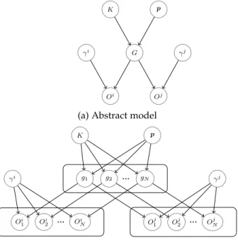
Fig. 2. Graphical model of the factors affecting the structure, data, and experts’ opinions (G: graph structure;D: data;O: experts’ opinions;p: prior distribution over edge types;K: information that determines G; γ: accuracy of experts; : noise). See text for further explanation.
and experts’ opinions O. In this model, K denotes the
set of information determining the structure. Note that the prior distribution p can be seen as a part of K, but we separate it because it plays a distinguished role in the next section. According to this model, data is directly affected by the structure and a noise factor. Experts’ opinions are also directly affected by the graph structure and experts’ accuracy parameters.
Fig.3shows graphical models of the experts’ opinions. The right model represents a more detailed version of the left one. According to this figure, the opinions of each expert are determined by the graph structure and the individ-ual’s accuracy parameters. More precisely, according to the detailed model, the opinion of one expert regarding one particular node pair is influenced by the edge status of that pair and the experts’ accuracy parameters.
Fig.4indicates the roles of different accuracy parameters of an expert in determining the personal opinions. In this figure,OiEandOAi are the opinions of theith expert about
the existing and absent edges inG, respectively. Based on this model, the opinions regarding existing edges are influ-enced byγ1andγ2parameters, and the opinions regarding absent edges are influenced by theγ3parameter.
Using the d-separation rules in Bayesian networks, in-troduced in Section 2, we can derive a set of conditional independence statements from these models. Some of these
statements are presented in Table 1. Only those used in
the remainder of the paper are listed here, as clearly, more statements can be read off from the graphical models. In each of the statements in Table1, assume that1≤i, j≤R, 1≤x, y≤N,i6=j, andx6=y.
There is one point that must be noted about the
in-dependence statements in Table 1. Consider statement 3
as an example. According to this statement, D and γ are
independent given G. Note that based on Fig. 2, if O is not given,Dandγ are independent, regardless of whether
G is given or not. Anyway, having G does not violate
this independence, and because we needD⊥γ |G in the
subsequent sections, we introduce this statement instead of
D⊥γ. This also holds for some other statements in Table1.
4
E
XPLICIT-A
CCURACY-B
ASEDS
COREIn our first scoring function, we explicitly use the estimated accuracy parameters of experts to quantify the quality of
γi
Oi G
Oj γj
p
K
(a) Abstract model
Oi
1 O
i
2 ... O
i N
p
K
Oj1 O
j
2 ... O
j N γi g1 g2 ... gN γj
(b) Detailed model
Fig. 3. Graphical models of the experts’ opinions.
γi
1, γi2
Oi E
G
Oi A
γi
3
Fig. 4. Graphical model of the roles of different accuracy parameters.
TABLE 1
Some Independence Statements Derived from Models of Figs.2to4
Number Statement Model
1 G⊥γ Fig.2
2 G⊥γ|p Fig.2
3 D⊥γ|G Fig.2
4 O⊥D|G Fig.2
5 O⊥D|G,γ Fig.2
6 Oi⊥Oj|G Fig.3a 7 Oi⊥Oj|G,γ
Fig.3a
8 Oj⊥γi|G, γj
Fig.3a
9 Ojx⊥Ojy|G, γj Fig.3b 10 Ojx⊥gy|gx, γj Fig.3b 11 Oi
x⊥O j
x|gx,p,γ Fig.3b 12 Ojx⊥γi|gx,p, γj Fig.3b 13 Ojx⊥p|gx, γj Fig.3b 14 (γ1, γi i
2)⊥γ3i Fig.4
4.1 Score Derivation
The goal of the explicit-accuracy-based scoring function is to score a candidate structureG using the dataD, experts’ opinionsO, and estimated experts’ accuraciesγ. A Bayesian measure of the goodness of fit ofGis its posterior probabil-ity givenD,O, andγ:
P(G|D, O,γ)∝P(G, D, O,γ) =
P(γ)P(G|γ)P(D|G,γ)P(O|G, D,γ).
Since P(γ) does not depend on the graph structure, we omit it from the score. P(G|γ) is simplified to P(G) based on statement 1 in Table 1. In addition,P(D | G,γ) is simplified to P(D | G) according to statement 3. Fi-nally, P(O | G, D,γ) is simplified to P(O | G,γ) using statement5. Therefore, the explicit-accuracy-based score is introduced as thelogofP(G|D, O,γ)and given as:
Scoreexplicit(G;D, O,γ)
= logP(G) + logP(D|G) + logP(O|G,γ). (1)
For the first two parts of this score, there are different choices mentioned in the literature. For the priorP(G), the simplest and most common choice, which we also use in our experiments, is the uniform prior. It means that all structures are equally likely a priori, and therefore we can omit it from the score. Other choices are to provide greater penalty to dense networks [24] and to consider the number of options in determining the parents of each node [25]. For the second part logP(D | G), we use the BDeu score introduced in Section2.
For the last part of the explicit-accuracy-based score, we use statements7,8,9,10from Table1and obtain
logP(O|G,γ) = R X
j=1
N X
i=1
logP(Oji |gi, γj). (2)
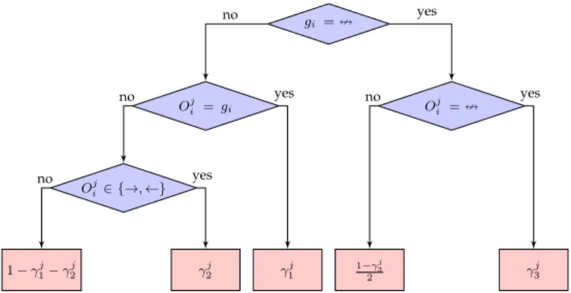
The termP(Oji |gi, γj)in equation (2) is computed using
the decision tree depicted in Fig.5. Note that we only use the provided opinions (i.e.,Oij 6= ∅) to scoreG. The reason for dividing 1−γ3j
by 2 in this figure is that when the
expert is wrong about an absent edge in G like X = Y,
he/she selects one of the possible edgesX→Y orX←Y. We consider these two possibilities equally likely because there is no evidence to favor one over the other.
4.2 Expectation-Maximization-Based Accuracy
Esti-mation
One way to estimate the experts’ accuracies is to use the expectation-maximization (EM) algorithm [26]. This ap-proach has been used in the crowdsourcing literatures such as [27], [28]. In the structure learning problem, we also previ-ously used this algorithm to estimate the experts’ confusion matrices [29], [30]. Here, we follow the same framework but derive the formulas for the three-parameter-based model of experts’ accuracies proposed in Section2.
If we consider the prior distributionpand the experts’
accuracies γ as the parameters, the maximum-likelihood
estimate of these parameters is
(ˆp,γˆ) = arg max
p,γ
{logP(O|p,γ)}.
Note that we use only the experts’ opinionsOin the likeli-hood function. Obviously, the dataDcan also help in this estimation problem, but we ignore it for simplicity’s sake.
To solve this optimization problem, we consider the true structureGas a hidden variable and use the EM algorithm. We assume that (Oi, gi) is independent of (Oj, gj), for
each j 6= i, given (p,γ). This assumption is not true in general, but to make the computations tractable, we ought to consider it. With this assumption, the log-likelihood of complete data(O, G)is
logP(O, G|p,γ) = N X
i=1
logP(Oi, gi|p,γ).
Sincegiis a member of{→,←,=}, we can write
logP(Oi, gi|p,γ)
= X
k∈{→,←,=}
I(gi=k) logP(Oi, gi=k|p,γ),
whereI(c)is the indicator function, which is one if the con-ditioncis satisfied and zero otherwise. We simply expand the inner term in the above expression as
P(Oi, gi=k|p,γ) =P(gi=k|p,γ)P(Oi|gi=k,p,γ).
Using statement2in Table1, we have
P(gi=k|p,γ) =P(gi =k|p) =pk. (3)
Also according to statement11in Table1, we have
P(Oi|gi =k,p,γ) = R Y
j=1
P(Oji |gi=k,p,γ). (4)
Finally, based on statements12 and13in Table1, the term in the above equation is simplified to
P(Oji |gi=k,p,γ) =P(Oji |gi=k, γj),
which is simply computed using the decision tree in Fig.5. Again, note that we consider only the provided opinions (i.e.,Oji 6=∅) in the computations.
Putting all the above together, the log-likelihood of com-plete data is
logP(O, G|p,γ) = N X
i=1
X
k∈{→,←,=}
I(gi=k)
×
logpk+ R X
j=1
logP(Oij|gi =k, γj)
. (5)
gi ==
Oj
i =gi Oij==
Oji∈ {→,←}
1−γj1−γ j
2 γ
j
2 γ
j 1
1−γj 3
2 γ
j 3
no yes
no yes
no yes
no yes
Fig. 5. Decision tree for computingP(Oij|gi, γj)forOji 6=∅.
The conditional expectation of the complete log-likelihood (5) given opinionsOand the current estimate of the parametersp(t),γ(t)is
Eη[logP(O, G|p,γ)] = N X
i=1
X
k∈{→,←,=}
Eη[I(gi=k)]
×
logpk+ R X
j=1
logP(Oij|gi =k, γj)
, (6)
where we denoteEG|O,p(t),γ(t)byEηfor the ease of reading.
The expectation of the indicator function is the probabil-ity of the associated event. Therefore,
Eη[I(gi=k)] =P(gi=k|O,p(t),γ(t)).
To make the computation of the above probability tractable, we assume that
P(gi =k|O,p(t),γ(t)) =P(gi =k|Oi,p(t),γ(t)).
This informally means that the status of the edge between two particular nodes is independent of the opinions regard-ing other node pairs, given the opinions about that node pair. This assumption means that that experts offer opin-ions about individual edges without taking opinopin-ions about other edges into account. It is based on assuming limited understanding of the semantics of Bayesian networks, quite common in domain experts of real-life problems.
Based on the above assumption and using Bayes’ rule, we have
Eη[I(gi=k)]
= P(gi=k|p
(t),γ(t))×P(O
i|gi=k,p(t),γ(t)) P(Oi|p(t),γ(t))
. (7)
The numerator terms can be computed using equa-tions (3) and (4), respectively, and the denominator is simply a normalization factor.
The next estimates of parameters are obtained by maxi-mizing the expectation (6). By setting the partial derivatives
of (6) with respect to each parameter equal to zero, we obtain the following estimates for the parameters:
p(kt+1)= 1
N N X
i=1
Eη[I(gi=k)],
(γ1j)(t+1)=
PN i=1
P
k∈{→,←}Eη[I(gi =k)]×I(O j i =k) PN
i=1
P
k∈{→,←}Eη[I(gi=k)]×I(Oji 6=∅) ,
(γ2j) (t+1)
= PN
i=1
P
k∈{→,←}Eη[I(gi=k)]×I(Oji6=k,O j
i∈{→,←})
PN i=1
P
k∈{→,←}Eη[I(gi=k)]×I(Oji6=∅) ,
(γ3j)(t+1)=
PN
i=1Eη[I(gi==)]×I(Oij==) PN
i=1Eη[I(gi==)]×I(O
j i 6=∅)
, (8)
fork∈ {→,←,=}and1≤j≤R.
In summary, the EM-based accuracy estimation algo-rithm works as follows:
(i) Take initial estimates of the parametersp,γ.
(ii) Use equation (7) and the current estimates of the pa-rameters to calculate estimates of the expectation of the hidden variablesgi.
(iii) Use equations (8) to obtain new estimates of the pa-rameters.
(iv) Repeat steps (ii) and (iii) until the results converge. The EM algorithm yields only local optima, but the con-siderable experience with the algorithm indicates that the results are usually satisfactory.
5
M
ARGINALIZATION-B
ASEDS
COREThe scoring approach proposed in the previous section con-sists of two steps. In the first step, the experts’ accuracies are estimated, then in the second step, the estimated accuracies are used to score the structures. Obviously, the reliability of this score depends on the reliability of the estimated accuracies in the first step. When we are not confident about the estimated accuracies, this approach is not appropriate. In this section, we introduce an alternative approach that is based on marginalizing out the accuracy parameters instead of explicitly estimating them.
Since the estimated experts’ accuracies are not explicitly used in the marginalization-based score, only the data D
structureG. The posterior probability ofGgivenDandO
is a reasonable measure for this purpose:
P(G|D, O)∝P(G, D, O) =P(G)P(D|G)P(O|G, D).
Based on the statement 4 in Table 1, P(O | G, D)
is simplified as P(O | G). Therefore, we define our
marginalization-based score as:
Scoremarg(G;D, O) = logP(G)+logP(D|G)+logP(O|G).
Comparing the above scoring function with the explicit-accuracy-based score (1), the only difference is the last term. In the rest of this section, we explain how to
com-pute logP(O | G) to complete the computation of the
marginalization-based score.
According to statement6in Table1,
logP(O|G) = R X
i=1
logP(Oi|G). (9)
To compute P(Oi | G), we marginalize out the accuracy parameters:
P(Oi|G) =
Z 1
0
Z 1−γi
1
0
Z 1
0
P(γ1i, γ2i, γ3i |G)
×P(Oi|γ1i, γ
i
2, γ
i
3, G)
dγi3dγ
i
2dγ
i
1. (10)
Note that the domain of integration forγ2i is not[0,1]but is [0,1−γ1i], becauseγ1i+γ2imust be lower than or equal to1.
According to statements1and14in Table1,
P(γi1, γ
i
2, γ
i
3|G) =P(γ
i
1, γ
i
2)P(γ
i
3). (11)
In addition, based on statement9we have
P(Oi|γi1, γi2, γ3i, G) =
N Y
j=1
P(Oji |γi1, γ2i, γ3i, G),
which can be written as
P(Oi|γi1, γ
i
2, γ
i
3, G)
= (γ1i)ni1(γ2i)ni2(1−γ1i−γi2)ni3(γ3i)mi1
1−γ3i 2
mi2 ,
(12)
where
• ni1 is the number of existing edges in G that are
detected by expertiwith correct directions,
• ni2 is the number of existing edges in G that are
detected by expertiwith reverse directions,
• ni3 is the number of existing edges in G that are
mentioned as absent edges by experti,
• mi1is the number of absent edges inGthat are correctly detected by experti,
• mi2 is the number of absent edges inGthat are men-tioned as existing edges by experti.
Plugging equations (11) and (12) into equation (10), we get
P(Oi|G) =
Z 1
0
P(γ3i) (γ
i
3)
mi1
1−γ3i 2
mi2 dγ3i
× Z 1
0
Z 1−γi
1
0
P(γi1, γ
i
2) (γ
i
1)
ni1(γi
2)
ni2
(1−γ1i−γi2)ni3dγ2idγ1i
. (13)
We denote the components of the above equation byI1i and
I2, respectively:i
I1i =
Z 1
0
P(γ3i) (γ3i)mi1
1−γi3 2
mi2 dγ3i,
I2i=
Z 1
0
Z 1−γi
1
0
P(γ1i, γ2i) (γ1i)ni1(γi2)ni2
(1−γ1i−γ
i
2)
ni3
dγi2dγ
i
1.
An appropriate distribution for P(γ3i)in I1i is the Beta distribution. If the shape parameters of this distribution are denoted byβi1andβi2, we have
P(γ3i) = 1
B(βi1, βi2) (γi3)
βi1−1(1−γi
3)
βi2−1,
(14)
where
B(βi1, βi2) =
Z 1
0
tβi1−1(1−t)βi2−1dt
(15)
is the Beta function. Note that the shape parameters can be different for different experts. Nevertheless, we use the same parameters for all experts in our experiments.
Plugging equation (14) into the definition ofI1, we havei
I1i =
R1 0(γ
i
3)βi1+mi1−1(1−γ3i)βi2+mi2−1dγ3i 2mi2×B(β
i1, βi2)
,
which can be written as
I1i =
B(βi1+mi1, βi2+mi2) 2mi2×B(β
i1, βi2)
. (16)
After deriving a closed-form formula for I1, we nowi turn our attention to I2. We use a Dirichlet distributioni Dir(αi1, αi2, αi3)forP(γ1i, γ2i):
P(γ1i, γ
i
2) = (γ1i)αi1
−1(γi
2)αi2
−1(1−γi
1−γi2)αi3
−1
B(αi1, αi2, αi3)
,
where B(αi1, αi2, αi3) is the multivariate Beta function. Using this prior in the definition ofI2i we have
I2i =
1
B(αi1, αi2, αi3)
Z 1
0
(γ1i)αi1+ni1
−1
× "
Z 1−γi
1
0
(γ2i)
αi2+ni2−1(1−γi
1−γ
i
2)
αi3+ni3−1dγi
2
# dγ1i.
Changing the variabletin integral (15) toγ2i by
substi-tuting t = γ
i
2
1−γi
1, the inner integral in the above equation
is
Z 1−γi
1
0
(γ2i)
αi2+ni2−1(1−γi
1−γ
i
2)
αi3+ni3−1dγi
2=
B(αi2+ni2, αi3+ni3)×(1−γ1i)
TABLE 2
Description of the Networks Used in the Simulation Experiments
Name Description Nodes Edges
Asia Diagnosing some respiratory diseases 8 8 Insurance Evaluating car insurance risks 27 52 Alarm Monitoring patients in intensive care 37 46 Hailfinder Predicting summer hails in northern Colorado 56 66
and therefore,
I2i =
B(αi2+ni2, αi3+ni3)
B(αi1, αi2, αi3)
× Z 1
0
(γ1i)αi1+ni1−1(1−γi1)αi2+ni2+αi3+ni3−1dγ1i,
which can be written as
I2i =
1
B(αi1, αi2, αi3)
×B(αi2+ni2, αi3+ni3)
×B(αi1+ni1, αi2+ni2+αi3+ni3). (17)
Based on equation (13), we can computeP(Oi | G)by multiplying equations (16), (17). So,
logP(Oi |G) = logB(βi1+mi1, βi2+mi2)
−mi2log 2−logB(βi1, βi2)
+ logB(αi1+ni1, αi2+ni2+αi3+ni3)
+ logB(αi2+ni2, αi3+ni3)
−logB(αi1, αi2, αi3).
Finally, based on equation (9) we getlogP(O | G)by summing the above expression fori= 1, . . . , R, which com-pletes the computation of the marginalization-based score.
6
E
XPERIMENTSThe developed scores are evaluated in this section using simulated experts (subsection6.1) and real experts (subsec-tion6.2).
6.1 Simulation Experiments
To evaluate the developed scores, some of the experiments are performed on simulated experts. The merit of simulation is that we can change the values of different parameters, such as the experts’ accuracies or the amount of available knowledge, and evaluate the scores under different condi-tions. In this part of the paper, we present the setup of our simulation experiments and discuss the obtained results.
6.1.1 Experimental Setup
We use four Bayesian networks which have been widely used in the structure learning experiments: Asia [31], Insur-ance [32], Alarm [33], and Hailfinder [34], briefly described in Table2.
Our experiments are implemented in a MATLAB en-vironment using the Bayes net toolbox [35] and the BNT structure learning package [36]. For each network, we gen-erate the data samples and experts’ opinions and learn the structure using different scoring functions. Comparing the learned network with the gold-standard structure reveals
TABLE 3
The Accuracy Parameters Assigned to Experts in Simulated Populations
Weak Mediocre Good
γ1 γ2 γ3 γ1 γ2 γ3 γ1 γ2 γ3
1 0.15 0.80 0.85 0.15 0.80 0.85 0.15 0.80 0.85 2 0.30 0.30 0.30 0.30 0.30 0.30 0.30 0.30 0.30 3 0.75 0.10 0.90 0.75 0.10 0.90 0.75 0.10 0.90 4 0.40 0.25 0.50 0.40 0.25 0.50 0.85 0.05 0.85 5 0.45 0.35 0.45 0.45 0.35 0.45 0.70 0.15 0.80 6 0.55 0.20 0.60 0.55 0.20 0.60 0.75 0.15 0.70 7 0.20 0.15 0.50 0.20 0.15 0.95 0.20 0.15 0.95 8 0.33 0.33 0.33 0.90 0.05 0.80 0.90 0.05 0.80 9 0.50 0.30 0.40 0.70 0.20 0.70 0.70 0.20 0.70 10 0.30 0.50 0.30 0.60 0.30 0.65 0.80 0.10 0.90 Mean 0.39 0.33 0.51 0.50 0.27 0.67 0.61 0.21 0.78
the effectiveness of the corresponding scoring function. In addition to comparing the DAGs, we also compare the CPDAGs representing the equivalence classes of the learned structure and the gold-standard network [21]. The reason for comparing the CPDAGs is that we do not penalize for structural differences that cannot be distinguished only based on data [37].
There may be three types of errors in the learned DAG (CPDAG):
• Wrong Connection where an absent edge in the original
graph is available in the learned network,
• Missed Edge where an available edge in the original
graph is missed in the learned structure,
• Wrong Orientation where one edge has different
orien-tations in the original graph and the learned structure.
Note that, when comparing two CPDAGs such asG1
andG2, if one edge is undirected inG1and directed in
G2, this is also considered as wrong orientation error, since there is at least one graph in the equivalence
class of G1 where its corresponding edge has wrong
orientation than that ofG2.
The total number of these errors is called the structural Hamming distance (SHD) [37], [38].
In our simulations, we consider three different
popu-lations each with R = 10 experts. According to the
ex-perts’ accuracies, these populations are labeled as “weak”,
“mediocre” and “good”. Table 3 lists the details of the
experts’ accuracies in these populations. Three experts are equally accurate in all populations. Three other experts are equally accurate in the “weak” and “mediocre” populations, but more accurate in the “good” population. The next three experts are equally accurate in the “mediocre” and “good” populations, but less accurate in the “weak” population.
Note that since higher γ1 and γ3 means more accurate
experts, these parameters have higher values in the “good” population. On the other hand, since higherγ2 means less accurate experts, this parameter has higher values in the “weak” population.1
In our experiments, we compare six different functions: 1) Data: This function neglects the experts’ opinions and
only uses the data D to score the structures. We use the marginal likelihood part of the BDeu score [2], introduced in Section2, for this purpose.
TABLE 4
The True Probability Distributions Over Edge Types for the Bayesian Networks Used in the Simulation Experiments
BN p→ p← p=
Asia 0.11 0.18 0.71 Insurance 0.07 0.08 0.85 Alarm 0.04 0.03 0.93 Hailfinder 0.02 0.02 0.96
2) Expert: This function neglects the dataDand only uses the experts’ opinions O to decide about the Bayesian network structure. It uses a majority voting approach, in which, for each pair (X, Y), the status that the majority of experts agree on is considered as the status of the edge between X and Y. In the case of a tie, a random decision is made.
3) PE: Stands for perfect experts, this scoring function assumes that all experts are completely accurate. For this, the explicit-accuracy-based score (1) is used, where
γ1 andγ3 parameters of all experts are set to one, and
γ2is zero.
4) Mean: This function also exploits both data and experts’ opinions using the explicit-accuracy-based score (1). It considers the same accuracies for all ex-perts to resemble the method proposed in [16]. For the accuracy parameters, it uses the mean of true ac-curacy parameters of all experts in each population. More precisely, if the opinions are generated from the “weak” population, γ1, γ2, γ3 are set to 0.4, 0.35, 0.5, respectively. For the “mediocre” population, these pa-rameters are set to 0.5, 0.25, 0.65, respectively. Finally, for the “good” population, 0.6, 0.2, 0.8 are used as the accuracy parameters for all experts. This scoring function is included in the experiments to compare the best achievable results from a method such as [16] that considers the same accuracy levels for all experts with the methods such as the EM-based method proposed in Section4 which try to estimate the accuracies of all experts.
5) EM: In this function, we first estimate the experts’ accuracies using the EM-based algorithm introduced in subsection4.2, and then, score the structures using the explicit-accuracy-based score (1). As the initial prior
distribution over edge types, we use p = {p→ =
0.1, p← = 0.1, p= = 0.8}, since we know that most real world Bayesian network structures are sparse. The true distributions for the used Bayesian networks are presented in Table4. For the initial accuracy parameters γ, we assume that we have the mean of true accuracy parameters of all experts a priori, and therefore, we initializeγ with the values used for the Mean scoring function. We use these initial values because we want to provide the same prior information for both Mean and EM scores, and can fairly compare their results. The EM algorithm stops when the absolute change in the estimated accuracies is smaller than 0.001.
6) Marg: This function is the marginalization-based
score introduced in Section 5. For the parameters
βi1, βi2, αi1, αi2, αi3, we use the same values for all
experts, again using the mean of true accuracy
param-eters. If the mean of true accuracy parameters of all experts in a particular population is¯γ1,¯γ2,γ¯3, we have
βi1=cγ¯3, βi2 =c(1−γ¯3),
αi1=cγ¯1, αi2=c¯γ2, αi3=c(1−γ¯1−¯γ2), (18)
for i = 1, . . . , R, where c is a constant coefficient. In the following, wherever the value of c is not clearly mentioned, its value is 10. At the end of this section, we evaluate the influence of this coefficient and show that its value does not have such a considerable impact on the obtained results.
In all of the above scoring functions, for the log-likelihoodlogP(D|G), the corresponding component from the BDeu score is used, and the parameter representing the equivalent sample size is set to 1. For the prior distribution over structures P(G), the uniform prior is used. Finally, as the search procedure, we use the same hill-climbing search as [2] introduced in Section2, starting from an empty network.
The number of opinions is controlled by a parameter
ν∈[0,1]. If there areNpairs of variables andRexperts, the total number of opinions provided by all experts is equal toround(ν×R×N), where the functionround(x)outputs the closest integer tox. In our experiments, the value of the parameterνis selected from{0.3,0.4,0.5,0.6}.
For the training dataset D, two different sizes are con-sidered: 1000 and 5000. To reduce the effect of randomness in the reported results, we repeat each experiment 10 times and report the average results over these iterations. In other words, for each Bayesian network, we generate 10 different datasets with 1000 samples and 10 different datasets with 5000 samples; and for each triple{Bayesian network, pop-ulation,ν}, we simulate 10 different opinion sets. Then, in each experiment, we use one dataset and one opinion set to learn the Bayesian network structure.
6.1.2 Results and Discussion
Tables 5 to 8 show the obtained structural Hamming
dis-tances for the Asia, Insurance, Alarm, and Hailfinder net-works, respectively. Each table includes three subtables, one for each population. In each row, the best obtained results are indicated by boldface values.
According to these tables, we observe that:
• The results obtained for theExpertscenario show that
using only the experts’ opinions gives rise to very low-accurate networks, especially for large networks and
weakpopulations. The main reason is that, in our experi-ments in accordance with the real world, the experts are not forced to present their opinions regarding all parts of the network, and we do not have enough information to accurately decide about the parts of the network that the majority of the experts are silent about.
• For theweakpopulations, the second worst results (after
theExpertscenario) are related to thePEscenario. The reason is that when there are considerable errors in the provided experts’ opinions, the raw usage of these opinions (as in thePEscenario) reduces the accuracy of the learned network.
• The third worst results for the weak populations are
scores which try to explicitly use the estimated experts’ accuracies, if the estimation process is not successful, it is not so useful to use the experts’ knowledge based on the explicit-accuracy-based score. This is the case for theEM-basedscenario for theweakpopulations. In fact, it is well known that the EM algorithm depends on the starting point and may converge to a local optimum. On the other hand, for theweak populations, the starting points are really questionable (which is why we call them weak). Therefore, the EM-based method fails to obtain robust results for theweakpopulations.
• In the majority of cases for the mediocre and good
populations, the EM-based method obtains either the
best or the second best results. This is because, in these situations, the EM algorithm starts with good enough starting points. The conclusion is that, when we are faced with accurate enough experts’ opinions, theEM-basedmethod obtains reasonable results. It may be asked, what if we do not know anything about the accuracy level of the opinions at hand? TheEM-based
method may get stuck in a local optimum far from true experts’ accuracies. This was the main stimulus for proposing an alternative approach, the marginalization-basedscoring function, in Section 5. It is clear from the tables that themarginalization-basedscore obtains more robust results.
• In the majority of cases for the weak populations, the marginalization-basedscore yields better results than the other scores. On the other hand, in situations where themarginalization-basedscore is not the winner, it ob-tains acceptable results compared to the best achieved results. Therefore, if we have no idea about the ac-curacy levels of our experts, it is better to use the
marginalization-basedscore.
• In the majority of cases for themediocreand good
pop-ulations, the results obtained by the EM-based score are superior to those obtained by theMeanscore. This shows that if we can successfully estimate the experts’ accuracies, using these estimated values for different experts is better than considering a constant accuracy level for all experts.
• One may think that with larger training datasets (e.g., |D| = 5000 in comparison with |D| = 1000), the structural Hamming distances will become smaller. However, this is not always the case. It can be explained by noting that learning Bayesian networks aims at two goals: (1) to obtain the structure of the domain, and (2) to obtain the probability distribution underlying the do-main. These two goals are sometimes in conflict: adding an extra edge to a Bayesian network may increase the structural Hamming distance, yet resulting in a more accurate probability distribution. This is sometimes the case with larger datasets, where complex networks with more wrong connections are preferred over the true net-work, yielding a more accurate probability distribution. There is some literature that supports this claim [16], [39]. In these situations, the experts’ opinions can be really useful to obtain more accurate structures of the domain, such as for the Hailfinder network in the Table8.
TABLE 5
The Obtained Structural Hamming Distances for the Asia Network
(a) Weak population
DAG CPDAG
|D| ν Data Expert PE Mean EM Marg Data Expert PE Mean EM Marg
1000
0.3 7.2 13.6 12.0 6.8 12.7 6.7 7.0 14.4 12.3 6.2 13.5 6.5 0.4 7.2 11.2 11.0 6.0 8.7 5.7 7.0 12.3 12.1 5.9 9.0 5.3
0.5 7.2 11.1 9.4 5.0 9.2 3.8 7.0 12.2 10.2 5.2 10.3 4.1
0.6 7.2 12.0 8.8 4.3 7.3 3.9 7.0 13.7 10.0 4.4 8.4 4.5 Avg 7.2 12.0 10.3 5.5 9.5 5.0 7.0 13.2 11.2 5.4 10.3 5.1
5000
0.3 9.3 13.6 10.5 6.9 10.3 7.4 9.5 14.4 10.9 7.0 11.0 7.7 0.4 9.3 11.2 9.2 5.4 7.6 4.9 9.5 12.3 9.9 4.6 7.6 4.5
0.5 9.3 11.1 9.3 5.2 9.2 3.8 9.5 12.2 10.2 5.1 9.9 3.9
0.6 9.3 12.0 8.8 4.5 7.1 4.1 9.5 13.7 10.0 4.1 7.6 3.4
Avg 9.3 12.0 9.5 5.5 8.5 5.1 9.5 13.2 10.3 5.2 9.0 4.9
(b) Mediocre population
DAG CPDAG
|D| ν Data Expert PE Mean EM Marg Data Expert PE Mean EM Marg
1000
0.3 7.2 8.6 4.7 3.9 5.0 2.8 7.0 9.9 5.3 3.8 5.0 2.6
0.4 7.2 7.6 5.2 5.1 5.5 4.3 7.0 8.6 5.6 4.7 5.5 4.4
0.5 7.2 5.1 3.0 2.8 3.3 1.7 7.0 6.4 2.9 2.1 3.2 1.1
0.6 7.2 4.4 2.7 2.1 2.8 1.3 7.0 5.8 3.7 1.9 3.1 1.2
Avg 7.2 6.4 3.9 3.5 4.2 2.5 7.0 7.7 4.4 3.1 4.2 2.3
5000
0.3 9.3 8.6 4.6 3.4 5.1 2.6 9.5 9.9 4.7 2.8 4.8 2.0
0.4 9.3 7.6 5.4 4.7 4.4 4.7 9.5 8.6 5.6 4.0 4.3 4.2 0.5 9.3 5.1 2.9 2.5 3.6 1.8 9.5 6.4 2.6 2.7 3.6 1.9
0.6 9.3 4.4 2.7 3.1 2.2 2.1 9.5 5.8 3.1 2.6 2.3 2.0
Avg 9.3 6.4 3.9 3.4 3.8 2.8 9.5 7.7 4.0 3.0 3.8 2.5
(c) Good population
DAG CPDAG
|D| ν Data Expert PE Mean EM Marg Data Expert PE Mean EM Marg
1000
0.3 7.2 5.7 4.2 4.4 3.9 3.2 7.0 7.6 4.9 4.3 4.4 2.6
0.4 7.2 4.6 2.0 3.3 2.6 2.0 7.0 5.4 2.3 3.1 2.7 1.8
0.5 7.2 3.7 1.2 2.2 0.9 1.1 7.0 5.1 1.4 2.2 1.2 1.1
0.6 7.2 2.4 1.1 0.9 0.9 0.9 7.0 4.0 1.1 0.4 0.7 0.7 Avg 7.2 4.1 2.1 2.7 2.1 1.8 7.0 5.5 2.4 2.5 2.3 1.6
5000
0.3 9.3 5.7 3.9 3.9 4.2 3.5 9.5 7.6 4.1 3.5 4.4 2.8
0.4 9.3 4.6 2.8 4.1 2.2 2.7 9.5 5.4 3.0 3.6 2.0 2.3 0.5 9.3 3.7 1.4 1.2 0.8 0.3 9.5 5.1 1.3 0.7 1.1 0.1
0.6 9.3 2.4 1.1 1.2 1.1 0.9 9.5 4.0 0.7 0.6 1.0 0.5
Avg 9.3 4.1 2.3 2.6 2.1 1.9 9.5 5.5 2.3 2.1 2.1 1.4
TABLE 6
The Obtained Structural Hamming Distances for the Insurance Network
(a) Weak population
DAG CPDAG
|D| ν Data Expert PE Mean EM Marg Data Expert PE Mean EM Marg
1000
0.3 29.2 126.9 53.9 29.6 36.9 28.0 36.6 132.0 61.6 36.8 43.1 36.0
0.4 29.2 107.0 49.9 28.0 29.1 23.3 36.6 114.5 58.1 36.1 34.7 28.9
0.5 29.2 108.2 49.5 31.1 28.6 29.0 36.6 115.0 56.6 39.4 36.6 34.7
0.6 29.2 104.0 50.3 30.0 30.6 25.7 36.6 110.2 57.2 36.6 39.1 34.8
Avg 29.2 111.5 50.9 29.7 31.3 26.5 36.6 117.9 58.4 37.2 38.4 33.6
5000
0.3 24.8 126.9 41.8 27.4 33.9 28.6 22.8 132.0 51.7 30.2 41.6 30.4 0.4 24.8 107.0 37.7 26.0 27.1 27.3 22.8 114.5 47.0 29.9 34.2 31.2 0.5 24.8 108.2 39.8 28.7 27.6 30.0 22.8 115.0 46.7 34.5 32.7 35.3 0.6 24.8 104.0 39.9 28.0 27.1 26.5 22.8 110.2 48.2 29.4 31.5 31.9 Avg 24.8 111.5 39.8 27.5 28.9 28.1 22.8 117.9 48.4 31.0 35.0 32.2
(b) Mediocre population
DAG CPDAG
|D| ν Data Expert PE Mean EM Marg Data Expert PE Mean EM Marg
1000
0.3 29.2 74.0 27.2 21.0 21.5 22.8 36.6 82.8 36.1 26.1 28.1 32.0 0.4 29.2 63.3 23.6 21.9 20.6 18.8 36.6 72.2 31.5 32.1 28.4 26.5
0.5 29.2 56.0 20.9 24.6 22.8 22.7 36.6 65.1 24.8 31.5 31.3 28.7 0.6 29.2 49.5 21.8 26.2 16.7 23.2 36.6 58.4 30.3 32.7 24.5 30.0 Avg 29.2 60.7 23.4 23.4 20.4 21.9 36.6 69.6 30.7 30.6 28.1 29.3
5000
0.3 24.8 74.0 21.0 19.1 21.5 19.6 22.8 82.8 28.5 21.1 25.0 22.4 0.4 24.8 63.3 22.3 24.1 24.5 20.9 22.8 72.2 29.2 28.7 26.4 24.9 0.5 24.8 56.0 20.6 26.7 21.6 20.7 22.8 65.1 26.2 30.2 26.1 24.6 0.6 24.8 49.5 21.0 23.7 16.1 19.7 22.8 58.4 27.7 27.0 19.2 24.8 Avg 24.8 60.7 21.2 23.4 20.9 20.2 22.8 69.6 27.9 26.8 24.2 24.2
(c) Good population
DAG CPDAG
|D| ν Data Expert PE Mean EM Marg Data Expert PE Mean EM Marg
1000
0.3 29.2 57.7 18.3 21.9 18.7 19.4 36.6 67.9 25.6 30.7 24.5 26.1 0.4 29.2 43.5 13.6 19.2 14.9 17.3 36.6 54.3 21.2 27.3 21.9 26.3 0.5 29.2 28.7 7.9 21.1 14.3 19.0 36.6 41.1 11.9 27.7 21.3 25.4 0.6 29.2 20.4 5.5 16.2 12.6 13.9 36.6 29.9 7.9 23.8 19.0 19.6 Avg 29.2 37.6 11.3 19.6 15.1 17.4 36.6 48.3 16.6 27.4 21.7 24.4
5000
0.3 24.8 57.7 19.7 22.4 16.9 19.4 22.8 67.9 27.1 27.0 20.9 22.3 0.4 24.8 43.5 14.0 18.5 12.8 18.6 22.8 54.3 18.8 18.8 14.9 20.2 0.5 24.8 28.7 12.7 19.1 9.7 17.4 22.8 41.1 18.0 24.4 12.9 21.5 0.6 24.8 20.4 8.2 16.3 9.4 13.8 22.8 29.9 11.5 21.3 10.0 15.6 Avg 24.8 37.6 13.7 19.1 12.2 17.3 22.8 48.3 18.9 22.9 14.7 19.9
TABLE 7
The Obtained Structural Hamming Distances for the Alarm Network
(a) Weak population
DAG CPDAG
|D| ν Data Expert PE Mean EM Marg Data Expert PE Mean EM Marg
1000
0.3 30.2 212.7 108.6 31.2 44.7 28.9 31.9 213.7 110.5 34.8 47.5 31.3
0.4 30.2 186.6 98.7 34.3 34.0 28.2 31.9 188.2 100.3 37.5 38.9 32.1 0.5 30.2 173.2 93.1 31.2 33.0 28.1 31.9 174.3 95.1 32.2 36.2 31.1
0.6 30.2 166.5 94.0 29.4 28.9 26.0 31.9 167.8 96.0 31.1 33.5 31.2 Avg 30.2 184.8 98.6 31.5 35.1 27.8 31.9 186.0 100.5 33.9 39.0 31.4
5000
0.3 29.5 212.7 83.8 29.9 38.4 28.4 30.5 213.7 87.0 33.2 41.3 30.5
0.4 29.5 186.6 79.9 31.1 31.5 27.8 30.5 188.2 83.0 34.0 34.9 30.5
0.5 29.5 173.2 77.0 30.2 32.6 24.8 30.5 174.3 78.9 30.9 35.0 28.3
0.6 29.5 166.5 76.8 27.0 26.4 24.8 30.5 167.8 78.8 29.6 29.0 28.0
Avg 29.5 184.8 79.4 29.6 32.2 26.5 30.5 186.0 81.9 31.9 35.0 29.3
(b) Mediocre population
DAG CPDAG
|D| ν Data Expert PE Mean EM Marg Data Expert PE Mean EM Marg
1000
0.3 30.2 123.0 61.8 29.1 30.5 25.3 31.9 125.5 65.7 32.7 34.8 29.4
0.4 30.2 95.9 48.6 28.0 21.7 23.4 31.9 98.7 51.8 30.6 25.3 26.0 0.5 30.2 87.0 43.7 29.9 21.9 28.1 31.9 89.3 47.0 33.0 24.3 32.2 0.6 30.2 78.5 38.1 22.5 15.6 17.6 31.9 81.1 40.1 26.8 17.8 20.3 Avg 30.2 96.1 48.1 27.4 22.4 23.6 31.9 98.7 51.1 30.8 25.5 27.0
5000
0.3 29.5 123.0 52.5 27.7 26.9 26.2 30.5 125.5 56.8 30.5 30.5 31.0 0.4 29.5 95.9 42.1 28.5 20.5 22.0 30.5 98.7 46.5 31.6 23.1 24.5 0.5 29.5 87.0 41.9 28.8 24.2 29.8 30.5 89.3 45.6 31.5 26.8 33.1 0.6 29.5 78.5 36.9 22.3 17.2 19.5 30.5 81.1 40.3 25.2 19.1 22.0 Avg 29.5 96.1 43.4 26.8 22.2 24.4 30.5 98.7 47.3 29.7 24.9 27.7
(c) Good population
DAG CPDAG
|D| ν Data Expert PE Mean EM Marg Data Expert PE Mean EM Marg
1000
0.3 30.2 87.9 38.3 21.7 17.6 17.6 31.9 90.6 42.4 25.8 21.3 21.5 0.4 30.2 62.4 26.5 20.8 16.1 18.0 31.9 65.4 28.7 25.1 19.6 21.1 0.5 30.2 37.7 13.3 16.3 8.2 10.6 31.9 40.8 15.0 19.6 10.0 12.1 0.6 30.2 36.1 15.1 15.7 8.8 9.0 31.9 39.8 17.3 18.8 9.6 11.2 Avg 30.2 56.0 23.3 18.6 12.7 13.8 31.9 59.2 25.8 22.3 15.1 16.5
5000
0.3 29.5 87.9 33.4 20.2 15.5 14.6 30.5 90.6 37.5 24.0 18.3 18.3
0.4 29.5 62.4 26.2 19.8 16.8 17.2 30.5 65.4 29.2 23.3 20.7 21.1 0.5 29.5 37.7 13.3 11.5 8.1 9.1 30.5 40.8 16.6 14.2 9.7 10.8 0.6 29.5 36.1 15.6 15.5 7.4 10.4 30.5 39.8 18.6 18.4 8.9 12.7 Avg 29.5 56.0 22.1 16.8 11.9 12.8 30.5 59.2 25.5 20.0 14.4 15.7
TABLE 8
The Obtained Structural Hamming Distances for the Hailfinder Network
(a) Weak population
DAG CPDAG
|D| ν Data Expert PE Mean EM Marg Data Expert PE Mean EM Marg
1000
0.3 67.0 409.5 79.1 40.6 48.0 35.0 70.1 415.9 84.4 45.5 52.5 40.5
0.4 67.0 399.9 86.4 44.2 45.1 36.3 70.1 405.5 92.3 48.9 49.7 41.5
0.5 67.0 375.3 85.5 45.0 45.0 44.3 70.1 380.9 92.2 48.9 49.2 48.7
0.6 67.0 367.6 90.3 44.2 46.1 36.1 70.1 374.1 96.7 49.4 51.3 41.5
Avg 67.0 388.1 85.3 43.5 46.0 37.9 70.1 394.1 91.4 48.2 50.7 43.1
5000
0.3 69.4 409.5 65.2 36.3 45.6 28.9 71.2 415.9 70.5 37.9 48.5 30.3
0.4 69.4 399.9 71.1 40.4 42.8 30.4 71.2 405.5 74.8 42.3 44.2 31.5
0.5 69.4 375.3 72.9 42.5 40.9 39.3 71.2 380.9 76.1 44.3 41.8 41.5
0.6 69.4 367.6 71.5 41.2 38.7 30.9 71.2 374.1 77.6 44.8 40.0 32.8
Avg 69.4 388.1 70.2 40.1 42.0 32.4 71.2 394.1 74.8 42.3 43.6 34.0
(b) Mediocre population
DAG CPDAG
|D| ν Data Expert PE Mean EM Marg Data Expert PE Mean EM Marg
1000
0.3 67.0 282.6 57.4 37.2 34.3 30.0 70.1 291.3 62.1 41.5 38.7 35.6
0.4 67.0 196.6 43.0 33.4 31.3 27.5 70.1 206.3 47.4 39.5 37.6 33.1
0.5 67.0 191.2 45.3 31.4 27.7 26.9 70.1 200.0 48.5 36.1 33.2 32.8
0.6 67.0 158.1 39.0 32.2 29.5 30.5 70.1 168.3 46.2 38.6 36.1 36.7 Avg 67.0 207.1 46.2 33.6 30.7 28.7 70.1 216.5 51.1 38.9 36.4 34.6
5000
0.3 69.4 282.6 50.8 31.6 27.4 22.1 71.2 291.3 55.4 34.8 28.6 23.2
0.4 69.4 196.6 36.0 26.4 23.1 16.2 71.2 206.3 39.4 28.6 24.8 17.7
0.5 69.4 191.2 37.0 24.0 16.3 16.2 71.2 200.0 43.1 25.9 17.2 18.3 0.6 69.4 158.1 33.7 24.5 22.7 21.3 71.2 168.3 35.6 26.5 24.9 23.3
Avg 69.4 207.1 39.4 26.6 22.4 19.0 71.2 216.5 43.4 29.0 23.9 20.6
(c) Good population
DAG CPDAG
|D| ν Data Expert PE Mean EM Marg Data Expert PE Mean EM Marg
1000
0.3 67.0 169.7 34.7 30.2 26.9 27.7 70.1 180.0 38.8 36.0 32.8 33.6 0.4 67.0 150.3 32.7 29.3 25.6 27.4 70.1 161.2 38.0 34.3 31.1 32.9 0.5 67.0 95.2 22.7 27.5 23.4 24.2 70.1 108.4 27.3 33.7 29.5 30.3 0.6 67.0 63.2 17.1 24.4 21.7 22.5 70.1 75.9 21.5 30.6 27.8 28.6 Avg 67.0 119.6 26.8 27.9 24.4 25.5 70.1 131.4 31.4 33.7 30.3 31.4
5000
0.3 69.4 169.7 30.7 22.1 19.2 18.3 71.2 180.0 32.7 24.5 20.7 20.5
0.4 69.4 150.3 26.7 20.8 16.1 18.8 71.2 161.2 29.7 22.6 17.1 20.6 0.5 69.4 95.2 19.2 17.5 13.5 13.1 71.2 108.4 21.4 19.6 15.6 15.4
0.6 69.4 63.2 11.7 13.5 11.5 11.9 71.2 75.9 12.3 16.0 13.6 14.0 Avg 69.4 119.6 22.1 18.5 15.1 15.5 71.2 131.4 24.0 20.7 16.8 17.6
results for Asia and Alarm networks as two representative examples. In Tables 5 and7, the value of the coefficient c
for the marginalization-based score is set to 10. Here, we repeat the same experiment for three completely different
TABLE 9
The Obtained Structural Hamming Distances Using the Marginalization-Based Score with Different Values of
Coefficientcfor Asia and Alarm Bayesian Networks
(a) Weak population
Asia BN Alarm BN
ν/c 0.1 1 10 100 0.1 1 10 100 0.3 7.7 7.5 6.7 6.5 29.4 29.4 28.9 29.0 0.4 5.5 5.3 5.7 6.0 28.7 29.3 28.2 32.4 0.5 4.2 4.0 3.8 5.0 29.5 29.3 28.1 29.3 0.6 4.6 4.3 3.9 4.4 28.9 26.8 26.0 25.8 Avg 5.5 5.3 5.0 5.5 29.1 28.7 27.8 29.1
(b) Mediocre population
Asia BN Alarm BN
ν/c 0.1 1 10 100 0.1 1 10 100 0.3 3.7 3.1 2.8 3.5 24.3 24.9 25.3 27.3 0.4 4.1 4.3 4.3 4.9 22.2 21.3 23.4 24.4 0.5 1.8 1.4 1.7 2.3 28.6 27.6 28.1 27.9 0.6 3.1 2.5 1.3 1.9 22.0 19.0 17.6 21.0 Avg 3.2 2.8 2.5 3.2 24.3 23.2 23.6 25.2
(c) Good population
Asia BN Alarm BN
ν/c 0.1 1 10 100 0.1 1 10 100 0.3 3.9 3.2 3.2 3.2 20.2 18.4 17.6 18.6 0.4 3.4 2.0 2.0 2.3 15.7 16.7 18.0 17.5 0.5 1.4 0.5 1.1 1.4 10.6 10.6 10.6 12.5 0.6 0.9 1.1 0.9 0.6 12.3 8.1 9.0 12.6 Avg 2.4 1.7 1.8 1.9 14.7 13.5 13.8 15.3
values from the set{0.1,1,100}. Table9shows the obtained structural Hamming distances between the learned struc-tures using the marginalization-based score and the original DAGs. Clearly, the accuracy of the marginalization-based score does not vary substantially when changing the value ofc.
6.2 Real World Experiments
To assess whether our methods of expert-opinion-guided structure learning actually work in practice, we have carried out an experiment with real experts. This experiment grew out of our work in computer-aided diagnosis of breast cancer using Bayesian networks [40], [41]. The field of concern was the interpretation of X-ray images by clinical radiologists, in particular X-ray images of breasts, referred to as mammograms. Our previous research has shown that this task can be done by means of a Bayesian network. We expected that the radiologists would be able to draft the structure of a Bayesian network, reflecting their knowledge of mammogram interpretation, depending on their experi-ence with the task. The radiologists had varying amounts of experience in this task: from more than 20 years of specialized experience to no specialized experience at all. Of course, all radiologists have some knowledge of mam-mogram interpretation.
Eight radiologists were asked to fill in the adjacency ma-trix shown in Table10and seven of them responded to the request.2 Three of the radiologists were experienced breast
TABLE 10
Table that the Radiologists had to Fill in as Part of the Experiment. Entries in the Upper Triangular Part of the Table had to be Filled in by→,←,=, or Remain Empty if
the Radiologists had no Idea what to Fill in
Micr
ocalcifications
Spiculation Location Age Lymph
Nodes
Skin
Retraction
Shape Size Br
east
cancer
Fibr
ous
T
issue
Develop
Br
east
Density
Mar
gin
Nipple
Dischar
ge
Ar
chitectural
Distort
Metastasis Mass
Microcalcifications Spiculation Location Age Lymph Nodes Skin Retraction Shape Size Breast cancer Fibrous Tissue Develop Breast Density Margin Nipple Discharge Architectural Distort Metastasis Mass
TABLE 11
The Accuracy Parameters and the Volume of Opinions Provided by Different Experts in the Breast Cancer
Experiment
Accuracy Parameters Volume of Opinions
γ1 γ2 γ3 number ratio
1 0.17 0.06 0.93 120 1
2 0.44 0.11 0.72 120 1
3 0.50 0.08 0.50 34 0.28
4 0.50 0.17 0.73 120 1
5 0.59 0.24 0.61 104 0.87
6 0.75 0.17 0.63 60 0.5
7 0.91 0.09 0.56 43 0.36
Avg 0.55 0.13 0.67 85.86 0.72
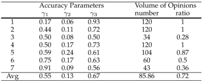
radiologists and also had ample experience as screening radiologists; two were starting breast and screening radi-ologists, and two were screening radiologists but no breast radiologists. The accuracy parameters and the number and ratio of provided opinions by these experts are presented in Table11.
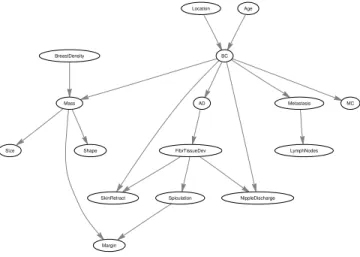
In our previous research, we have designed several Bayesian network structures in collaboration with experi-enced radiologists. These radiologists were different from the radiologists we asked for our current experiment. None of the radiologists had ever seen one of the Bayesian net-works we had designed previously. One of those netnet-works
is shown in Fig.6. The Bayesian network model combines
clinical features with radiological examination by X-rays. In addition, the Bayesian network integrates the results of microcalcification analysis, which is a separate image analysis procedure.
Training data was generated from the Bayesian network shown in Fig.6, which is considered as the gold-standard structure.3Table12shows the obtained structural Hamming distances between the gold-standard structure and the struc-tures learned using the scoring functions mentioned in sub-section6.1.1. In this table,|D|means the number of training data which is selected from the set{100,400,700,1000}. In order to reduce the effect of randomness in the reported
3. This Bayesian network is available at http://www.cs.ru.nl/ ∼peterl/teaching/CI/networks/bc.net.
TABLE 12
The Obtained Structural Hamming Distances for the Breast Cancer Network with Real Experts
|D| Data Expert PE Mean EM Marg 100 13.2 32.0 26.4 9.7 25.3 10.2 400 8.5 32.0 23.4 7.2 19.6 7.2
700 6.8 32.0 22.0 5.8 18.2 5.8
1000 6.8 32.0 21.0 5.8 17.9 5.8
Avg 8.8 32.0 23.2 7.1 20.3 7.3
results, each experiment is repeated 10 times (for 10 different training datasets) and the average results over these repeti-tions are reported. Finally, the coefficientcin equation (18) for the marginalization-based score is set to 100.
As it is clear from Table12, the Mean and Marg scoring functions obtained the best results. The success of Mean scoring function is due to the low variance in the experts’ accuracies. More precisely, according to Table11, the accu-racies of different experts are not so far from the average values and therefore, using these average values instead of individual accuracies yielded good results.
Although Mean and Marg scores obtained similar results
in Table12, we now show that our marginalization-based
scoring function is more reliable. Note that both functions need an estimation of the average experts’ accuracies as in-put. These average values are used as the individual experts’ accuracies in the Mean function, and for calculating the parameters βi1, βi2, αi1, αi2, αi3 using equation (18) in the Marg function. Obviously, in real world applications, there might be some errors in the estimated average accuracies. To compare Mean and Marg scoring functions, we studied the behaviors for different levels of errors in this input vector.
Fig.7shows the mean and one standard deviation error bars for the structural Hamming distances obtained from Mean and Marg scores. The horizontal axis is the available error in the input average accuracy vector, which is equal to the sum of the absolute errors in the input vector related to the true vector ([0.55,0.13,0.67]). According to this figure, in general, the marginalization-based score obtains lower structural Hamming distances with lower standard devia-tions, which shows the robustness of this function compared to the Mean scoring function.
7
C
ONCLUSIONThis paper focused on exploiting the opinions of multiple domain experts regarding the cause-effect relationships be-tween random variables for structure learning of Bayesian networks. The proposed approach enables structure learn-ing to exploit experts’ opinions to learn more accurate network structures than from data alone. Well-known lim-itations of structure learning algorithms, such as the huge, super-exponential size of the search space and the impossi-bility to distinguish between Markov-equivalent structures using data alone, motivated this research.
MC
Spiculation
Location Age
LymphNodes
SkinRetract Shape Size
BC
FibrTissueDev BreastDensity
Margin
NippleDischarge
AD Metastasis
Mass
Fig. 6. The structure of the Bayesian network for breast cancer diagnosis.
0 0.5 1 1.5 2 5
10 15 20
Input Error
SHD
Marg Mean
Fig. 7. The mean and one standard deviation error bars for the structural Hamming distances obtained from Mean and Marg scores as functions of the available error in the input average accuracy vector for the breast cancer network with real experts.
To exploit the provided opinions, we introduced two new scoring functions to be used in the score-based Bayesian network structure learning. The main novelty of the proposed scores is that we take into account the natural point of view that different experts have different individual probabilities of correctly labeling the inclusion or exclusion of edges in the structure. The accuracy of each expert was modeled by three parameters. In the first scoring function, the experts’ accuracies are first estimated using an expectation-maximization-based algorithm. Then, the es-timated values are explicitly used in the scoring process. When we are confident about the estimated accuracies, this scoring function results in robust decisions. On the other hand, when it is not possible to find a confident estimate of experts’ accuracies, our second score, the marginalization-based score, which marginalizes out the accuracy parame-ters results in more robust scores.
Some of the future research directions are (i) to work on relaxing the assumptions made in the development of the EM-based accuracy estimation algorithm described in Section 4.2, (ii) to develop algorithms that use data
along with experts’ opinions to obtain improved estimates of experts’ accuracies, (iii) to use the recently published agreement/disagreement algorithm [42] for estimating the experts’ accuracies in the structure learning problem, and (iv) to exploit the experts’ opinions for constraint-based structure learning. For example, the provided opinions can help to obtain more accurate conditional independencies.
A
CKNOWLEDGMENTWe would like to thank dr. Mechli Imhof-Tas from Rad-boudUMC, Nijmegen for her valuable help in gathering the opinions from the radiologists regarding the breast cancer network.
R
EFERENCES[1] G. F. Cooper and E. Herskovits, “A Bayesian method for the induction of probabilistic networks from data,”Machine learning, vol. 9, no. 4, pp. 309–347, 1992.
[2] D. Heckerman, D. Geiger, and D. M. Chickering, “Learning Bayesian networks: The combination of knowledge and statistical data,”Machine learning, vol. 20, no. 3, pp. 197–243, 1995.
[3] D. M. Chickering, “Optimal structure identification with greedy search,”The Journal of Machine Learning Research, vol. 3, pp. 507– 554, 2003.
[4] L. M. De Campos, “A scoring function for learning Bayesian networks based on mutual information and conditional indepen-dence tests,”The Journal of Machine Learning Research, vol. 7, pp. 2149–2187, 2006.
[5] C. P. De Campos and Q. Ji, “Efficient structure learning of Bayesian networks using constraints,”The Journal of Machine Learning Re-search, vol. 12, pp. 663–689, 2011.
[6] S. Huang, J. Li, J. Ye, A. Fleisher, K. Chen, T. Wu, E. Reiman, A. D. N. Initiativeet al., “A sparse structure learning algorithm for Gaussian Bayesian network identification from high-dimensional data,”Pattern Analysis and Machine Intelligence, IEEE Transactions on, vol. 35, no. 6, pp. 1328–1342, 2013.
[7] M. Studen `y and D. Haws, “Learning Bayesian network structure: Towards the essential graph by integer linear programming tools,” International Journal of Approximate Reasoning, vol. 55, no. 4, pp. 1043–1071, 2014.