Design and Implementation of the PULSAR Programming
System for Large Scale Computing
Jakub Kurzak1, Piotr Luszczek1, Ichitaro Yamazaki1, Yves Robert2,
Jack Dongarra1
c
The Authors 2017. This paper is published with open access at SuperFri.org
The objective of the PULSAR project was to design a programming model suitable for large-scale machines with complex memory hierarchies, and to deliver a prototype implementation of a runtime system supporting that model. PULSAR tackled the challenge by proposing a program-ming model based on systolic processing and virtualization. The PULSAR programprogram-ming model is quite simple, with point-to-point channels as the main communication abstraction. The runtime implementation is very lightweight and fully distributed, and provides multithreading, message-passing and multi-GPU offload capabilities. Performance evaluation shows good scalability up to one thousand nodes with one thousand GPU accelerators.
Keywords: runtime scheduling, dataflow scheduling, distributed computing, massively parallel computing, multicore processors, hardware accelerators, virtualization, systolic arrays.
Introduction
MotivationHigh-end supercomputers are on the steady path of growth in size and complexity. One can get a fairly reasonable picture of the road that lies ahead by examining the platforms that will be brought online under the DOEs CORAL initiative. In 2018, the DOE aims to deploy three different CORAL platforms, each over 150 petaflop peak performance level. Two systems, named Summit and Sierra, based on the IBM OpenPOWER platform with NVIDIA GPU-accelerators, were selected for Oak Ridge National Laboratory and Lawrence Livermore National Laboratory; an Intel system, based on the Xeon Phi platform and named Aurora, was selected for Argonne National Laboratory.
Summit and Sierra will follow the hybrid computing model, by coupling powerful latency-optimized processors with highly parallel throughput-latency-optimized accelerators. They will rely on IBM Power9 CPUs, NVIDIA Volta GPUs, and NVIDIA NVLink interconnect to connect the hybrid devices within each node, and a Mellanox Dual-Rail EDR Infiniband interconnect to connect the nodes. The Aurora system, on the contrary, will offer a more homogeneous model by utilizing the Knights Hill Xeon Phi architecture, which, unlike the current Knights Corner model, will be a stand-alone processor and not a slot-in coprocessor, and will also include integrated Omni-Path communication fabric. All platforms will benefit from recent advances in 3D-stacked memory technology.
Overall, both types of systems promise major performance improvements: CPU memory bandwidth is expected to be between 200 GB/s and 300 GB/s using HMC; GPU memory bandwidth is expected to approach 1 TB/s using HBM; GPU memory capacity is expected to reach 60 GB (NVIDIA Volta); NVLink is expected to deliver no less than 80 GB/s, and possibly as high at 200 GB/s, of CPU to GPU bandwidth. In terms of computing power, the Knights Hill is expected to be between 3.6 teraFLOPS and 9 teraFLOPS, while the NVIDIA Volta is expected to be around 10 teraFLOPS.
1University of Tennessee, Knoxville, USA
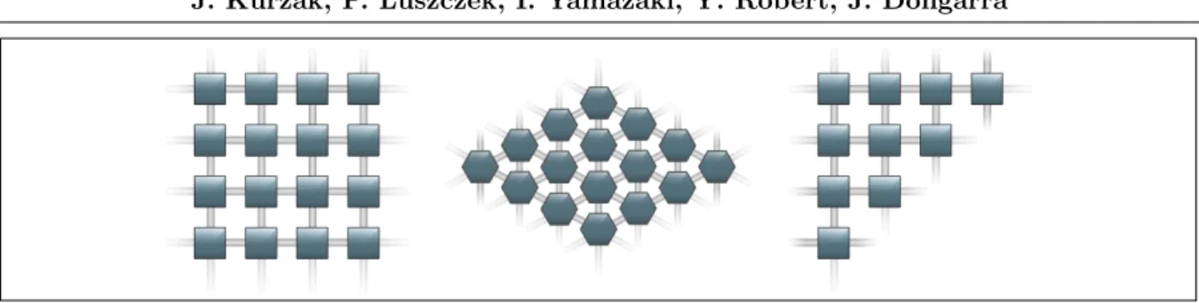
Figure 1. Canonical systolic array shapes
And yet, taking a wider perspective, the challenges are severe for software developers who have to extract performance from these systems. The hybrid computing model seems to be here to stay, and memory systems will become even more complicated. It is clear that support for parallelism is going to have to dramatically increase, going up by at least an order of magnitude for the CORAL systems and achieving billion-way parallelism at exascale. The PULSAR project attempts to tackle these challenges with a simple programming model, based on the systolic processing model, augmented with virtualization. The programming model is simple and so is the runtime implementation. Processing is completely distributed and, therefore, very scalable.
Background
Systolic arrays are descendants of array-like architectures such as iterative arrays, cellular automata and processor arrays. A systolic array is a network of processors that rhythmically compute and pass data through the system. The seminal paper by Kung and Leiserson [42] defines systolic arrays as devices with “simple and regular geometries and data paths” with
“pipelining as general methods of using these structures”.
The systolic array paradigm is a departure from the von Neuman paradigm. While the von Neuman architecture is instruction-stream-driven by an instruction counter, the systolic array architecture is data-stream-driven by data counters. A systolic array is composed of matrix-like rows of units called cells or Data Processing Units (DPUs). DPUs operation is transport-triggered, i.e., triggered by the arrival of a data object. The DPUs are connected in a mesh-like topology (often two-dimensional). Each DPU is connected to a small number of nearest neighbor DPUs and performs a sequence of operations on data that flows through it. Often different data streams flow across the mesh in different directions. Figure 1 shows three canonical shapes of systolic arrays: square can be used for a dense matrix multiplication,
diamond for a band matrix factorization, triangle for a dense matrix factorization.
Early on, Kung identified the main strength of systolic arrays as ability to addressing the problem of the I/O bottleneck: “Thus, a problem what was originally compute-bound can become I/O-bound during its execution. This unfortunate situation is the result of a mismatch between the computation and the architecture. Systolic architectures, which ensure multiple computations per memory access, can speed up compute-bound computations without increasing I/O require-ments” [41]. Other valuable properties of systolic arrays include highly scalable parallelism, modularity, regularity, local interconnection, high degree of pipelining, and highly synchronized multiprocessing.
computa-tional wavefronts in the algorithm, and pipelining these wavefronts on the processor array. The computing network serves as a data-wave-propagating medium.
The computational wavefronts are data-driven. In a sense, they are similar to electromag-netic wavefronts, since each processor acts as a secondary source and is responsible for the activation of the next front. Despite the lack of global timing, the sequencing of tasks is cor-rectly followed. Whenever data are available, the sender informs the receiver and the receiver accepts the data whenever required. This scheme can be implemented through a simple hand-shaking protocol, which ensures that the computational wavefronts propagate in an orderly manner. Wavefront arrays share the features of regularity, modularity, local interconnection, and pipelining: “A wavefront array equals a systolic array plus dataflow computing” [43].
Most importantly, computations expressed as aDirect Acyclic Graph(DAG) can be mapped to an array processor, by assigning multiple nodes of the DAG to each processing element, as long as the DAG is uniform (shift-invariant). Examples of algorithms, which belong to this class include: convolution, autoregressive filtering, discrete Fourier transforms and an array of dense linear algebra algorithms - matrix multiplication, LU factorization, QR factorization, triangular matrix inversion, and more.
The origins of systolic arrays can be traced back to parallel array computers such as the Solomon computer [29] and its successor ILLIAC IV [7, 40]. At the peak of interest in the mid 80s systolic arrays targeted special-purpose algorithm-oriented VLSI implementations, often as attached processors. The ideas also led to the design of theWarpmachines [3], which were a series of increasingly general-purpose systolic array processors created by Carnegie Mellon University in conjunction with industrial partners: G. E., Honeywell and Intel, and funded by the U. S.
Defense Advances Research Projects Agency (DARPA). Interest in systolic arrays died off by early 90s, mostly due to the high cost of implementing them as special-purpose hardware during a time in which Moore’s law was relentlessly increasing the computing power and decreasing the cost of general-purpose processors.
In their seminal paper [42], Kung and Leiserson applied systolic arrays to problems in dense linear algebra: matrix multiplication, Gaussian elimination, and triangular solve. They also pointed out applications in signal processing: convolution, Finite Impulse Response (FIR) filter, and discrete Fourier transform. A large body of work on systolic arrays was devoted to applications in dense linear algebra [1, 6, 8, 17, 28, 46, 56].
Despite the loss of interest in systolic arrays per se, systolic principles lead to a series of efficient algorithms for general-purpose computer systems, the prime example being a series of algorithms for matrix multiplication, including: Cannon’s [10], Fox’s [26], BiMMeR [30], PUMMA [16], SUMMA [58], and DIMMA [15].
The paper by Fisher and Kung [24] offers an extensive overview of systolic array literature. General discussion and motivation for systolic arrays is given by Kung [41], and Fortes and Wah [25]. Systematic treatment of the topic is provided by Robert [52, 53] and Evans [22]. The paper by Kung [43] coins the term wavefront arrays and discusses the mapping of task graphs to systolic architectures. The paper by Johnsson et al. [32] talks about general purpose systolic arrays that can be applied to a wider range of problems (reconfigurable computing).
Related Work
include the DARPA-sponsored HPCS (High Productivity Computing Systems) program [21] which stressed productivity rather than performance, with the latter being the prerequisite for the former. The older PGAS languages include Titanium [4, 19, 37–39, 44, 45, 50], UPC (Unified Parallel C) [11, 18], and CAF (Co-Array Fortran) [23, 51]. They use the concept of globally visible address space with an explicit handling of addresses that are non-local. The ongoing efforts in the Fortran community ensure continuous support for CAF functionality as exemplified by CAF 2.0 [31, 48, 49, 54] and incorporation of some of the CAF features into the Fortran 2008 standard [55]. The DARPA’s HPCS program introduced three more languages into the space: Fortress [2, 33], X10 [59], and Chapel (Cascade High Productivity Language) [12, 13]. The last two are still maintained by IBM and Cray, respectively. A recent resurgence of activity around shared memory programming resulted in the OpenSHMEM [14] project that borrows some ideas from the PGAS model, but is much more library-centric, as opposed to requiring a completely new programming language.
The other approach to achieving good performance on the current Petascale and future Exascale hardware designs is to use software runtime systems. Two notable projects in this cat-egory are Charm++ [36] and PaRSEC [9], which deal with algorithms and their implementation represented as a Direct Acyclic Graph (DAG) of tasks connected with edges that communicate data between them – a concept clearly related to the dataflow paradigm. Many other systems offer similar paradigm but might not afford the same type of support for distributed memory parallelism [5, 47].
A new execution model has been argued by the authors of ParalleX [27, 34, 35] and im-plemented by the HPX project [57] that now serves as a clear need for extensions of the C++ standard. Codelets Execution Model [20] can also be considered in the category of the new models of computation.
Outline
The rest of the paper is organized as follows. We describe the PULSAR programming model in Section 1, and further explain the construction and operation of a PULSAR instance in Section 2. We outline the runtime implementation in Section 3. Then the following sections are devoted to the detailed description of an example, namely Cannon’s algorithm. We briefly review the algorithm in Section 5 and report performance results in Section 6. Finally, we state some final remarks in Section 6.
1. Programming Model
The PULSAR programming model relies on five abstractions to define the computation:
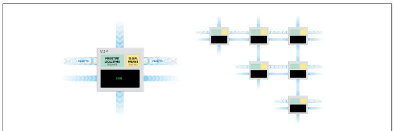
VSA, VDP, channel, packet, tuple; and on two abstractions to map the computation to the actual hardware: thread,device. Figure 2 conveys the basic ideas.
Virtual Systolic Array (VSA) A set of VDPs connected with channels.
Virtual Data Processor (VDP) The basic processing element in the VSA.
Channel A point-to-point connection between a pair of VDPs.
Packet The basic unit of information transferred in a channel.
Figure 2. A VDP (left) and a VSA (right)
Thread Synonymous with a CPU thread or an entire (multicore) CPU.
Device Synonymous with an accelerator device (GPU, Xeon Phi, etc.)
The sections to follow describe the roles of the different entities, how the VDP operation is defined, how the VSA is constructed, and how the VSA is mapped to the hardware. These oper-ations are accessible to the user through PULSAR’s Application Programming Interface(API). Because this API is quite small (12 core functions and 6 auxiliary functions), actual function names are used when describing the different actions. Currently, PULSAR is implemented in C and exports C bindings.
1.1. Tuple
Tuples are strings of integers. Each VDP is uniquely identified by a tuple. Tuples can be of any length, and different length tuples can be used in the same VSA. Two tuples are identical if they are of the same lengths and have identical values of all components. Tuples are created using the variadic function prt tuple new, which takes a (variable length) list of integers as its input. The user only creates tuples; after creation, the tuples are passed to VDP and channel constructors. They are destroyed by the runtime at the appropriate time of destroying those objects. As a general rule in PULSAR, the user only creates objects and loses their ownership after passing them to the runtime.
1.2. Packet
packet after pushing it to a channel. The packet can be used until theprt vdp packet release function is called.
1.3. Channel
Channels are unidirectional point-to-point connections between VDPs, used to exchange packets. Each VDP has a set of input channels and a set of output channels. Packets can be fetched from input channels and pushed to output channels. Channels in each set are assigned consecutive numbers starting from zero (or slots). Channels are created using the prt channel new function and providing tuples of source and destination VDPs, and slot num-bers in the source and destination VDPs. The user does not destroy channels. The runtime destroys channels at the time of destroying the VDP. After creation, the channel needs to be inserted in the appropriate VDP, using the prt vdp channel insertfunction. The user needs to insert a full set of channels to each VDP. At the time of inserting the VDP in the VSA, the system joins channels that identify the same communication path.
1.4. VDP
The VDP is the basic processing element of the VSA. Each VDP is uniquely identified by a tuple. The VDP is assigned a function which defines its operation. Within that function, the VDP has access to a set of global parameters, its private, persistent local storage, and its channels. The runtime invokes that function when there are packets in all of the VDP’s input channels. This is called firing. When the VDP fires, it can fetch packets from its input channels, call computational kernels, and push packets to its output channels. It is not required that these operations are invoked in any particular order. The VDP fires a prescribed number of times. When the VDP’s counter goes down to zero, the VDP is destroyed. The VDP has access to its tuple and its counter.
At the time of the VDP creation, the user specifies if the VDP resides on a CPU or on an accelerator. This is an important distinction, because the code of a CPU VDP has synchronous semantics, while the code of an accelerator VDP has asynchronous semantics. In other words, for a CPU VDP, actions are executed as they are invoked, while for an accelerator VDP, actions are queued for execution after preceding actions complete. In the CUDA implementation, each VDP has its own stream. All kernel invocations have to be asynchronous calls, placed in the VDP’s stream. Similarly, in the case of an accelerator VDP, all channel operations have asynchronous semantics.
1.5. VSA
The VSA contains all VDPs and their channel connections, and stores the information about the mapping of VDPs to the hardware. The VSA needs to be created first and then launched. An empty VSA is created using the prt vsa newfunction. Then VDPs can be inserted in the VSA using the prt vsa vdp insertfunction. Then the VSA can be executed using the prt vsa run function, and later destroyed using theprt vsa delete function.
prt packet t*packet=prt vdp packet new(vdp, ...);
kernel that writes(...,packet->data, ...);
prt vdp channel push(vdp,slot,packet);
prt vdp packet release(vdp,packet);
prt packet t*packet=prt vdp channel pop(vdp,slot);
kernel that modifies(...,packet->data, ...);
prt vdp channel push(vdp,slot,packet);
prt vdp packet release(vdp,packet);
prt packet t*packet=prt vdp channel pop(vdp,slot);
prt vdp channel push(vdp,slot,packet);
kernel that reads(...,packet->data, ...);
prt vdp packet release(vdp,packet);
for(v=0;v<vdps;v++){
prt vdp t*vdp=prt vdp new(...);
for(in=0;in<inputs;in++){
prt channel t*input=prt channel new(...);
prt vdp channel insert(vdp,input, ...);
}
for(out=0;out<outputs;out++){
prt channel t*output=prt channel new(...);
prt vdp channel insert(vdp,output, ...)
}
prt vsa vdp insert(vsa,vdp, ...);
}
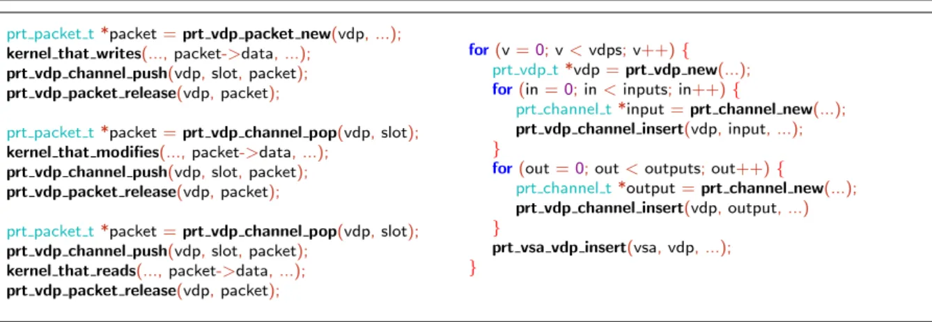
Figure 3. Code snippets for VDP operation (left) and VSA construction (right)
and another for mapping VDPs to devices. These functions have to return the global thread or device number, based on the VDP’s tuple and the total thread count or device count.
VSA construction can be replicated or distributed. The replicated construction is more straightforward from the user’s perspective. In the replicated construction, each MPI process inserts all the VDPs, and the system filters out the ones that do not belong in a given node, based on the VDP-to-thread and the VDP-to-device function. However, the VSA construction process is inherently distributed, so each process can also insert only the VDPs that belong in that process.
2. Construction and Operation
The VSA is first constructed, and then launched. The VSA is constructed by creating all VDPs and inserting them in the VSA. Each VDP, in turn, is constructed by creating all its channels and inserting then in the VDP. The operation of the VSA is defined through the operation of its VDPs. VDPs operate by launching computational kernels, and communicating by writing and reading packets to and from their channels.
2.1. VSA Construction and Launching
Figure 3 shows a simple code snippet for VSA construction. A VSA is created using the prt vsa newfunction, which returns a new VSA with an empty set of VDPs. After creation, the VSA has to be populated with VDPs. Then the VSA can be launched using the prt vsa run function. After execution, the VSA can be destroyed using the prt vsa delete function. The function destroys all resources associated with the VSA.
2.2. VDP Creation and Insertion
The user has to define the VDP function. The runtime invokes that function when packets are available in all of the VDP channels, which is calledfiring. Inside that function, the user has access to the VDP object. In particular, the user has access to its tuple, counter, local store and global store. global storeis the read-only global storage area, passed to the VSA at the time of its creation.local store is the VDP private local storage area, which is persistent between firings. tuple is the VDP unique tuple, assigned at the time of creation. counter is the VDP counter. At the first firing, the counter is equal to the value assigned at the time of the VDP creation. At each firing the counter is decremented by one. At the last firing the counter is equal one.
2.3. Channel Creation and Insertion
A channel is created using the prt channel new function. After creation, the channel can be inserted into the VDP using the prt vdp channel insertfunction. The user does not free the channel. At the time of calling prt vdp channel insert, the runtime takes ownership of the channel. The channel will be destroyed in the process of the VSA execution or at the time of calling prt vsa delete.
2.4. Mapping of VDPs to Threads and Devices
The user defines the placement of VDPs on CPUs and GPUs by providing the mapping function at the time of the VSA creation withprt vsa new. The runtime calls that function for each VDP and passes as parameters: the VDP tuple, the pointer to the global store, the total number of CPU threads at the VSA disposal in that launch, and the total number of devices in that launch.
The function has to return the mapping information in an object of type prt mapping t, with the fields location and rank, where the location can be either PRT LOCATION HOST or PRT LOCATION DEVICE, and the rank indicates the global rank of the unit.
2.5. VDP Operation
This section describes actions which can take place inside the VDP function, i.e., the function passed to prt vdp new. The user never calls that function; it is called by the runtime when packets are available in all active input channels of the VDP. Inside that function, computational kernel can be launched and packets can be created, deleted, pushed down output channels and fetched from input channels.
A new data packet can be created by calling theprt vdp packet newfunction and released by calling theprt vdp packet releasefunction. The runtime will keep the packet and its data around until it completes all pending operations associated with the packet. However, the packet and its data should not be accessed after the release operation.
2.6. Channel Deactivation and Reactivation
A channel can be deactivated by the VDP by calling the prt vdp channel off function. This indicates to the runtime that it can schedule the VDP (call the VDP function) without checking if there are packets in that channel. The VDP should not attempt to read packets from an inactive channel.
A channel can be reactivated by the VDP by calling theprt vdp channel onfunction. This indicates to the runtime that it cannot schedule the VDP (call the VDP function) if there are no incoming packets in that channel. By default, channels are active.
2.7. Handling of Tuples
A new tuple can be created by calling the variadic function prt tuple new. A tuple has to have at least one element. There is no upper limit on the number of elements. Tuples are dynamically allocated strings or integers, with the INT MAX constant at the end, serving as the termination symbol. As such, tuples can be freed by calling the C standard libraryfreefunction. However, tuples should not be freed after passing them to the PULSAR runtime. The runtime will free all such tuples during its operation or at the time of callingprt vsa delete.
3. Runtime Implementation
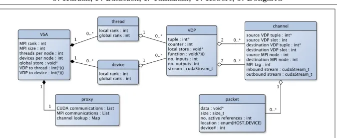
Figure 4 shows the main objects in the runtime implementation and their relations. The VSA is the top-level object containing multiple threads and devices, threads being synonymous with CPU cores, and devices being synonymous with accelerator devices. It also contains a single instance of the communication proxy, which is a server-like object responsible for managing inter-node (MPI) and intra-node (PCI) communication. Each thread and device maintains a list of multiple VDP. Each VDP maintains two separate lists of channels, one for input channels, one for output channels. Each channel maintains a list of packets.
In a CPU-only scenario, there may be no devices; in a GPU-only scenario, there may be no threads. Depending on the distribution of VDPs to threads and devices, any particular thread or device may end up with an empty list of VDPs. There may be VDPs with no input channels - pure data producers, as well as VDPs with no output channels - pure data consumers. In practical scenarios, most VDPs will have a number of input and output channels. A list of packets in a channel will grow and shrink at runtime.
3.1. Tuple
Tuples are implemented as strings of integers, terminated with the INT MAXmarker. Tuples support copy, concatenation and two types of comparisons. One checks for an exact match in size and content, the other implements lexicographical ordering.
3.2. Packet
Figure 4. Structure of PULSAR runtime
it to a channel, or it can push it to multiple channels to implement a broadcast or multi-cast operation.
While the packet is a very simple concept in the context of a CPU implementation, support for accelerators introduces an additional level of complexity, due to the fact that accelerators have separate memories. A shared-memory system with multiple accelerators basically looks to the programmer like a distributed-memory, global address space system. To handle this situation, PULSAR runtime keeps track of the location of the packet, which can be either in the host (CPU) memory, or in the memory of one of the accelerators. This is the reason a packet is not a stand-alone object, but is subordinate to a VDP. Packets are created by VDPs and inherit their initial locations from the VDPs that create them.
Another level of complexity is introduced by the fact that PULSAR cannot rely on CUDA functions for device memory allocations, without sacrificing asynchronous semantics, since CUDA allocations cannot be executed in a stream. Because of that, PULSAR implements its own device memory allocator, which grabs a large chunk of the device memory at the time of initialization, and assigns memory segments asynchronously at runtime. Currently, the imple-mentation is very simple, with fixed size (configurable) segments and fixed size (also configurable) initial reservation. PULSAR maintains one such allocator per device, and each packet maintains a reference to its allocator.
3.3. Channel
Channels are packet carriers between VDPs. A channel knows the tuples and slots of its source and destination VDPs, and maintains a list of packets. A channel also knows the numbers (MPI ranks) of the nodes, where the source and destination VDPs reside, as well as its unique tag for MPI communication between the pair of nodes it connects. A channel connecting to a device VDP is also assigned a unique stream to allow for asynchronous communication (one that does not block kernel launches).
VDPs are both CPU VDPs, residing in the same node, the operation is as simple as moving the packet from one queue to another. Things are more complicated if the channel crosses node boundaries, in which case MPI is invoked. Yet a different scenario is implemented if a boundary between a host memory and a device memory has to be crossed. And finally, the most complex case is invoked when a packet residing in device memory is sent across the network. The last case results in a sequence of CUDA callbacks and non-blocking MPI calls, initiated by the channel and carried out by the communication proxy, with support from the CUDA runtime and MPI. As an extension to the basic programming model, a channel contains an active/inactive
flag, which allows the VDP for suspending channel activities. By deactivating a channel, the VDP pledges to not pop packets from that channel, which allows the VDP to fire with that channel being empty. Newly created channels are active by default. A VDP can deactivate and re-activate channels at will, as long as it does not attempt to fetch packets from an inactive channel.
3.4. VDP
A VDP is the basic execution unit of the VSA. A VDP knows its tuple and counter, and the lists of input and output channels. It is assigned a function, local store and global store. Support for accelerators requires a VDP to also know its location, i.e., if it is assigned to a CPU or an accelerator, and which accelerator, if there are multiple of them in a node. An accelerator VDP is also assigned its unique stream, so that multiple VDPs can execute at the same time, in different streams, and also kernel launches can overlap data transfers.
In order to hide the complexity of managing the memory system within a single node (host plus multiple devices), the VDP provides more abstract functions for accessing lower-level functions of packets and channels. Specifially, rather than calling packet and channel methods directly, the user calls VDP methods to perform operations on packets and channels. E.g., to create a packet, the user calls the VDP function prt vdp packet new, so that the packet can inherit its initial location from the creator VDP. For consistency, a packet is released by the VDP upon calling the function prt vdp packet release. Similarly, channels are accessed by VDP functions prt vdp channel pushand prt vdp channel pop. First, this is consistent with the handling of packets. Second, the user designates channels by using their slot numbers, rather than references, which slightly increases the level of abstraction.
3.5. Threads and Devices
Threads and devices are internal PULSAR objects not directly accessed by the user. The user only deals with them indirectly by providing formulas for mapping of VDPs to threads and devices. Threads and devices know their local (within a node) and global ranks, and maintain lists of VDPs.
of controlling each GPU. This still leaves the problem with asynchronous communication and multi-stream execution.
The requirement for the GPU VDPs to only contain asynchronous calls allows for maximum performance and the simplest runtime implementation. A single CPU thread is sufficient to launch all the computation and communication to multiple GPUs, and in the actual PULSAR implementation, it is the same thread that is also responsible for all MPI transactions.
3.6. VSA
The VSA is the main object in PULSAR, containing all the top-level information about the system, including: the total number of nodes and the rank of the local node, the number of CPU threads launched per node, and the number of GPU devices used per node. It contains the lists of threads and devices, and the communication proxy. It also contains a number of auxiliary structures, like a lookup table of local VDPs, and a list of channels connecting the local node to other nodes, as well as the list of memory allocators for all local devices.
The most complicated function provided by the VSA is VDP insertion. First, the VSA evaluates the mapping function to find out the VDP location. VDPs that do not belong in the local node, are immediately discarded. VDPs that do belong in the local node, are inserted in the appropriate thread or device, depending on the location returned by the mapping function. Then local channels are merged. Each VDP is inserted with a complete set of channels. If the newly inserted VDP has channels connecting to other VDPs, inserted before, each pair of duplicate channels is merged into one channel. To support this operation, the VSA maintains a hash table, where the VDPs can be looked up by their tuples.
Then a unique (MPI) tag is assigned to each channel going out of the node. All channels connecting each pair of nodes have consecutive tags. This is necessary, because PULSAR im-plements VDP-to-VDP communication on top of MPI. MPI messages are received with the MPI ANY SOURCE, MPI ANY TAG flags and the destination VDP identified by the rank of the ori-gin and the tag of the channel. Consecutive numbering of tags connecting each pair of nodes, as opposed to, e.g., global numbering in the whole system, prevents the problem of exhausting the 16-bit tag size limit of older MPI implementations. To support this operation, the VSA maintains lists of channels connecting the local node to all other nodes.
Finally, at the time of inserting a device VDP, a unique stream is created and assigned to the VDP to enable its asynchronous operation.
At the time of launch, the VSA basically launches threads and waits for their completion. Each CPU thread carries out its own execution. For a CPU-only run, nothing more is required. If the run is distributed and/or accelerators are involved, the VSA launches an extra thread for the proxy, which carries out the firings of device VDPs, as well as the MPI and PCI communication.
3.7. Proxy
• Post another send for each agent. • Complete another send for each agent. • Post another receive.
• Complete another receive.
• Cycle each device, i.e., fire another VDP on each device. • Issue all local communications.
The most complicated transfer that may happen in the system is when a GPU sends a packet across the network. Figure 5 illustrates that situation. The following sequence of events takes place:
1. In the VDP function, the prt vdp channel pushfunction is called do push a packet down a channel. At this point, the packet resides in device memory. A CUDA callback is placed in the VDP stream, to trigger the transfer, when all preceding VDP operations complete. 2. CUDA runtime executes the callback, which places the transfer request in proxy’s list of
local requests.
3. The proxy handles the transfer request by placing asynchronous device-to-host memory copy, across the PCI, in the outbound stream associated with the channel performing the communication.
4. The proxy follows up with placing a callback in the channel’s outbound stream, to trigger a transfer across the network, when the PCI transfer completes.
5. CUDA runtime executes the callback, which places the transfer request in the proxy’s list of local requests.
6. The proxy places a send request in the list of sends requested by the device.
7. The proxy issues the MPI Isend action, and moves the request from the list of sends re-quested to the list of sends posted.
8. The proxy tests the send request for completion. When the request completes, the proxy removes the request from the list of sends posted and releases the packet.
A similar, although not identical, sequence of actions happens on the receiving side, where the message is received, the destination VDP identified, and appropriate steps taken depending on its location. Specifically, if the destination VDP resides in one of the devices, a transfer across the PCI is queued with the proxy. As long as the sequence is, there are no shortcuts here, since potentially two PCI buses and the network interface have to be crossed by the data. Little can be done about the latency of such transfers, however, all the emphasis in PULSAR is on latency hiding, rather than minimizing. The objective is to keep the buses and network interfaces saturated by multiple transfers going on at any given point in time.
4. Software Engineering
Although being an experimental project, PULSAR has a quite robust implementation. PUL-SAR is coded in C in a fairly object-oriented manner, and would be very suitable for a C++ implementation. PULSAR is very compact with only 21 .c files, 22 .h files and 6,600 lines of code. The compactness and clear structure is mostly thanks to the very crisp abstractions established in the design process (VDP, VSA, channel, packet, etc.)
proxy proxy CUDA
CUDA MPIMPI
MPI_Isend(
proxy->send_requests)
MPI_Test(
proxy->send_requests) queue_append(
proxy->local_requests, DEVICE->HOST->MPI)
queue_append(
proxy->send_requests, DEVICE->HOST->MPI) VDP
VDP
prt_vdp_channel_push cudaStreamAddCallback( vdp->stream,
DEVICE->HOST->MPI) queue_append(
proxy->local_requests, DEVICE->HOST->MPI)
cudaMemcpyAsync( cudaMemcpyDeviceToHost, channel->outbound_stream) cudaStreamAddCallback( channel->outbound_stream, DEVICE->HOST->MPI) 1
2
3
4
5
6
7
8
Figure 5.Timeline for a transfer originating from a GPU and involving MPI
the -DMPI flag in the compilation options and linking the application with an MPI library, in addition to the PULSAR library. The same goes for CUDA with the -DCUDAflag. At the same time, the use of#definedirectives is avoided thorughout the code. Instead of conditional blocks of code handling MPI and CUDA, the code is written as if MPI and CUDA were present. If they are not, a set of empty MPI/CUDA stub functions is included.
PULSAR only depends on the most basic data structures: a non-thread-safe double-linked list, a thread-safe double-liked list (implemented by protecting the non-thread-safe one with Pthread spinlocks), and a hash table. The basic linked list and hash table are implemented themselves as dependency-free, stand-alone structures.
PULSAR contains its own tracing routines, based on recording time of different events and writing an SVG file at the end of execution. PULSAR records computational tasks on CPUs and GPUs (VDP firings), MPI communications, and CUDA data transfers. CPU timestamps are taken using get time of day, GPU timestamps are take usingcudaEventRecord.
PULSAR code, including the runtime (PRT) and examples, is available on the project website (https://bitbucket.org/icl/pulsar), which also contains extensive documentation, including: installation instructions, users’ guide, reference manual, etc. The code is documented using Doxygen and the reference manual is produced automatically from Doxygen annotations. A simple version is available in HTML and an extended version in PDF, where function call graphs and data structures dependency graphs are also included.
5. Cannon’s Matrix Multiplication
processors is used to compute the matrix product, C =A×B, by rotating the A matrix from left to right, and the B matrix from top to bottom, while each processor computes a block of C.
Figure 6. Cannon’s matrix multiplication algorithm
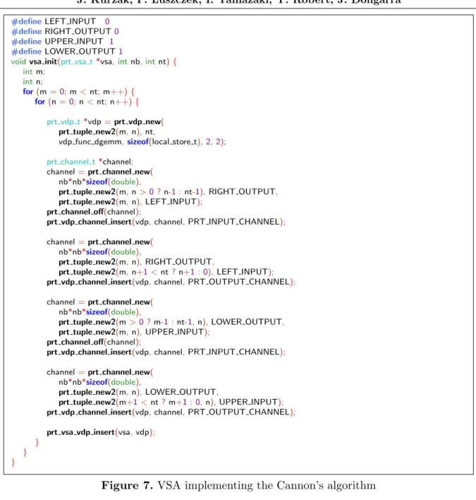
Figure 7 shows the PULSAR code for the construction of the VSA. The basic premise of the implementation is to built a 2D mesh of VDPs, and let each VDP compute one tile of the result matrix C. Herenbis the size of each tile, andntis the width and height of the matrix (number of tiles). The code loops over the vertical and horizontal dimensions of the matrix and, for each tile, creates a VDP, creates four channels (two vertical, two horizontal), inserts the channels in the VDP, and inserts the VDP in the VSA.
Each VDP holds its local tile of the C matrix, as well as its local tiles of matrices A and B, which are distributed in a skewed fashion, as depicted on Figure 6, i.e., tiles of the B matrix are shifted by one vertically, from column to column, and tiles of A are shifted by one horizontally, from row to row. All channels are initially inserted as inactive, so that each VDP can be launched without any data in the input channels, compute the local part of the product, send its local tile of A to the right, and send its local tile of B down.
Figure 8 shows a complete code of a VDP implementing the Cannon’s algorithm. It starts with the declarations section, where tile size (nb) and matrix size (nt) are retrieved from global store, the location of the VDP tile in the matrix (m, n) is retrieved from the VDP tuple, an alias is created to thelocal store. Thedonevariable is declared because the cuBLAS calls require passing of the constant by reference.
The first half of the code handles the first step, when the VDP’s counter equals to the size of the matrix. If the VDP is a device VDP (is assigned to a GPU), then cuBLAS initializations are handled in the first step (creating cuBLAS handle and associating it with the VDP’s stream). Then the local tile A is pushed to the right and the local tile of B is pushed down. Then the local product is computed, either using a cuBLAS call or a CBLAS call, depending on the VDP’s location. Finally, the input channels are activated to provide data for the next step.
#defineLEFT INPUT 0 #defineRIGHT OUTPUT0 #defineUPPER INPUT 1 #defineLOWER OUTPUT1
voidvsa init(prt vsa t*vsa,intnb,intnt){
intm;
intn;
for(m=0;m<nt;m++){
for(n=0;n<nt;n++){
prt vdp t*vdp=prt vdp new(
prt tuple new2(m,n),nt,
vdp func dgemm,sizeof(local store t),2,2);
prt channel t*channel; channel=prt channel new(
nb*nb*sizeof(double),
prt tuple new2(m,n>0?n-1:nt-1),RIGHT OUTPUT,
prt tuple new2(m,n),LEFT INPUT);
prt channel off(channel);
prt vdp channel insert(vdp,channel,PRT INPUT CHANNEL);
channel=prt channel new( nb*nb*sizeof(double),
prt tuple new2(m,n),RIGHT OUTPUT,
prt tuple new2(m,n+1<nt?n+1:0),LEFT INPUT);
prt vdp channel insert(vdp,channel,PRT OUTPUT CHANNEL);
channel=prt channel new( nb*nb*sizeof(double),
prt tuple new2(m>0?m-1:nt-1,n),LOWER OUTPUT,
prt tuple new2(m,n),UPPER INPUT);
prt channel off(channel);
prt vdp channel insert(vdp,channel,PRT INPUT CHANNEL);
channel=prt channel new( nb*nb*sizeof(double),
prt tuple new2(m,n),LOWER OUTPUT,
prt tuple new2(m+1<nt?m+1:0,n),UPPER INPUT);
prt vdp channel insert(vdp,channel,PRT OUTPUT CHANNEL);
prt vsa vdp insert(vsa,vdp);
} } }
Figure 7.VSA implementing the Cannon’s algorithm
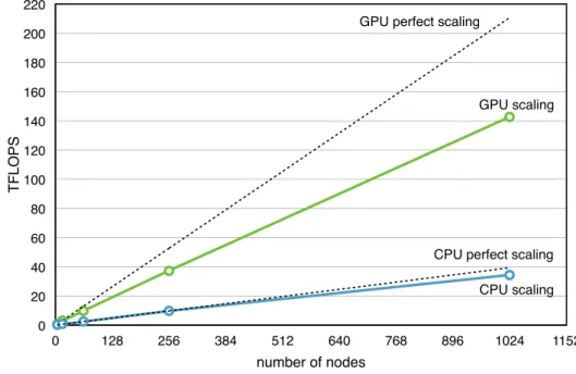
6. Performance Experiments
PULSAR’s capabilities are demonstrated using a simple weak scaling experiment carried out on up to 1024 nodes of the Titan supercomputer. Each node contains a 16-core AMD Interlagos CPU and one NVIDIA Tesla K20X GPU. In this experiment, the nodes are assigned in a square array of size 2×2, 4×4, 8×8, 16×16 and 32×32. Each node is assigned a 4×4 array of tiles, where each tile is of size 2048×2048. Runs are made using CPUs only or GPUs only. Multithreaded BLAS is used for the CPU runs and cuBLAS is used for the GPU runs.
voidvdp func dgemm(prt vdp t*vdp){
intnb= ((global store t*)vdp->global store)->nb;
intnt= ((global store t*)vdp->global store)->nt;
intm=vdp->tuple[0];
intn=vdp->tuple[1];
local store t*local store= (local store t*)vdp->local store;
doubledone=1.0;
// IF first step.
if(vdp->counter==nt){
// IF device VDP.
if(vdp->location==PRT LOCATION DEVICE){
cublasStatus tcublas status;
cublas status=cublasCreate(&local store->cublas handle);
cublas status=cublasSetStream(local store->cublas handle,vdp->stream);
}
// Push local A right.
prt packet t*right packet=prt vdp packet new(vdp,nb*nb*sizeof(double),local A);
prt vdp channel push(vdp,RIGHT OUTPUT,right packet);
// Push local B down.
prt packet t*lower packet=prt vdp packet new(vdp,nb*nb*sizeof(double),local B);
prt vdp channel push(vdp,LOWER OUTPUT,lower packet);
// Compute local AxB.
if(vdp->location==PRT LOCATION DEVICE){
cublasDgemm(local store->cublas handle,CUBLAS OP N,CUBLAS OP N,nb,nb,nb,
&done,local A,nb,local B,nb, &done,local C,nb);
}else{
cblas dgemm(CblasColMajor,CblasNoTrans,CblasNoTrans,nb,nb,nb,
1.0,local A,nb,local B,nb,1.0,local C,nb);
}
// Activate input channels.
prt vdp channel on(vdp,LEFT INPUT);
prt vdp channel on(vdp,UPPER INPUT);
}else{
// Move A horizontally.
prt packet t*left packet =prt vdp channel pop(vdp,LEFT INPUT);
if(vdp->counter>1)
prt vdp channel push(vdp,RIGHT OUTPUT,left packet);
// Move B vertically.
prt packet t*upper packet=prt vdp channel pop(vdp,UPPER INPUT);
if(vdp->counter>1)
prt vdp channel push(vdp,LOWER OUTPUT,upper packet);
// Compute AxB.
if(vdp->location==PRT LOCATION DEVICE){
cublasDgemm(local store->cublas handle,CUBLAS OP N,CUBLAS OP N,nb,nb,nb,
&done,left packet->data,nb,upper packet->data,nb, &done,local C,nb);
}else{
cblas dgemm(CblasColMajor,CblasNoTrans,CblasNoTrans,nb,nb,nb,
1.0,left packet->data,nb,upper packet->data,nb, 1.0,local C,nb);
}
// Release transient packets.
prt vdp packet release(vdp,left packet);
prt vdp packet release(vdp,upper packet);
} }
Figure 8.VDP code implementing the Cannon’s algorithm
In the CPU case, MPI communication is completely overlapped with computation, resulting in no gaps in the trace and almost idea scaling. In the GPU case, the DMA transfers do not keep up with the speed of execution, and the MPI transfers do not keep up with the DMA transfers, resulting in large gaps in the trace and poor scaling. At the same time, GPU execution still produces much higher overall performance than CPU execution.
1
4 0.823 0.823 0.153476875 0.153476875
16 2.897 3.292 0.611632845 0.6139075
64 9.992 13.168 2.450502888 2.45563
256 37.404 52.672 9.797182039 9.82252
1024 142.757 210.688 34.42743329 39.29008
0 20 40 60 80 100 120 140 160 180 200 220
0 128 256 384 512 640 768 896 1024 1152
T
F
L
O
PS
number of nodes
GPU perfect scaling
CPU scaling GPU scaling
CPU perfect scaling
Figure 9. Scaling of Cannon’s algorithm
CPUs MPI CPUs MPI CPUs MPI CPUs MPI node 1 node 2 node 3 node 4
Figure 10.CPU trace using 4 nodes
GPU DMA MPI GPU DMA MPI GPU DMA MPI GPU DMA MPI node 1 node 2 node 3 node 4
Figure 11.GPU trace using 4 nodes
Conclusion
This paper has presented the PULSAR system. PULSAR combines the key paradigms of systolic arrays (regularity, extensive data re-use and multilevel pipelining) with virtualization techniques, in order to provide a simple yet efficient programming model to design parallel algorithms on complex multicore systems with attached accelerators.
After detailing the nuts and bolts of the system, we have provided a comprehensive descrip-tion of a PULSAR instance, namely the canonic Cannon’s algorithm for matrix product. We have shown convincing performance results on Titan, which nicely demonstrate that a limited programming effort, as required by PULSAR, is not incompatible with an efficient implementa-tion. Achieving a good trade-off between the ease of programming and the quality of the results was the primary objective of PULSAR.
Acknowledgements
This work has been supported by the National Science Foundation, under grant SHF-1117062, Parallel Unified Linear algebra with Systolic ARrays (PULSAR). The authors would also like to thank the National Institute for Computational Sciences, the Georgia Institute of Technology and the Oak Ridge National Laboratory for generous computer allocations on their supercomputers. Yves Robert has been supported by Institut Universitaire de France.
This paper is distributed under the terms of the Creative Commons Attribution-Non Com-mercial 3.0 License which permits non-comCom-mercial use, reproduction and distribution of the work without further permission provided the original work is properly cited.
References
1. Ahmed, H.M., Delosme, J.M., Morf, M.: Highly concurrent computing struc-tures for matrix arithmetic and signal processing. Computer 15(1), 65–82 (1982), DOI: 10.1109/MC.1982.1653828
2. Allen, E., Culpepper, R., Nielsen, J., Rafkind, J., Ryu, S.: Growing a syntax. In: ACM SIGPLAN Foundations of Object-Oriented Languages workshop. ACM, Savannah, GA, USA (2009)
3. Annaratone, M., Arnould, E., Gross, T., Kung, H.T., Lam, M., Menzilcioglu, O., Webb, J.A.: The Warp computer: Architecture, implementation, and performance. IEEE Transac-tions on Computers C-36(12), 1523–1538 (1987), DOI: 10.1109/TC.1987.5009502
4. Arpaci, R., Culler, D., Krishnamurthy, A., Steinberg, S., Yelick, K.: Empirical evaluation of the CRAY-T3D: A compiler perspective. In: Proceedings of the 22nd Annual International Symposium on Computer Architecture. pp. 320–331. IEEE, Santa Margherita Ligure, Italy (June 22-24 1995), iSSN: 1063-6897, Print ISBN: 0-89791-698-0, INSPEC Accession Number: 5086797
6. Barada, H., El-Amawy, A.: Systolic architecture for matrix triangularisation with partial pivoting. IEE Proceedings E, Computers and Digital Techniques 135(4), 208–213 (1987), ISSN: 0143-7062
7. Barnes, G.H., Brown, R.M., Kato, M., Kuck, D.J., Slotnick, D.L., Stokes, R.A.: The ILLIAC IV computer. IEEE Transactions on Computers C-17(8), 746–757 (1968), DOI: 10.1109/TC.1968.229158
8. Bojanczyk, A.W., Brent, R.P., Kung, H.T.: Numerically stable solution of dense systems of linear equations using mesh-connected processors. SIAM J. Sci. Stat. Comput. 5(1), 95–104 (1984), DOI: 10.1137/0905007
9. Bosilca, G., Bouteiller, A., Danalis, A., Faverge, M., Haidar, H., Herault, T., Kurzak, J., Langou, J., Lemarinier, P., Ltaief, H., Luszczek, P., YarKhan, A., Dongarra, J.: Dis-tibuted Dense Numerical Linear Algebra Algorithms on Massively Parallel Architectures: DPLASMA. Tech. rep., Innovative Computing Laboratory, University of Tennessee (apr 2010),http://icl.cs.utk.edu/news_pub/submissions/ut-cs-10-660.pdf
10. Cannon, L.E.: A Cellular Computer to Implement the Kalman Filter Algorithm. Ph.D. thesis, Montana State University (1969)
11. Carlson, W.W., Draper, J.M., Culler, D.E., Yelick, K., Brooks, E., Warren, K.: Introduction to UPC and language specification. Tech. Rep. CCS-TR-99-157, CCS (May 13 1999)
12. Chamberlain, B., Callahan, D., Zima, H.: Parallel programmability and the chapel language. International Journal of High Performance Computing Applications 21(3), 291–312 (August 2007)
13. Chapel language specification 0.750 (2007), http://chapel.cs.washington.edu/spec-0. 750.pdf, accessed: 2017-02-15
14. Chapman, B., Curtis, T., Pophale, S., Koelbel, C., Kuehn, J., Poole, S., Smith, L.: In-troducing OpenSHMEM, SHMEM for the PGAS community. In: PGAS’10: The Fourth Conference on Partitioned Global Address Space Programming Models. PGAS, ACM, New York, NY, USA (October 12-15 2010)
15. Choi, J.: A new parallel matrix multiplication algorithm on distributed-memory concurrent computers. In: High Performance Computing on the Information Superhighway, 1997. HPC Asia ’97. pp. 224–229. IEEE, Seoul (April-May 1997), DOI: 10.1109/HPC.1997.592151
16. Choi, J., Walker, D.W., Dongarra, J.J.: PUMMA: parallel universal matrix multiplication algorithms on distributed memory concurrent computers. Concurrency Computat.: Pract. Exper. 6(7), 543–570 (1994), DOI: 10.1002/cpe.4330060702
17. Comon, P., Robert, Y.: A systolic array for computing BA−1. IEEE Trans-actions on Acoustics, Speech and Signal Processing 35(6), 717–723 (1987), DOI: 10.1109/TASSP.1987.1165208
19. Darcy, J.: Writing robust IEEE recommended functions in ”100% pure Java”(tm). Tech. Rep. CSD-98-1009, Computer Science Division, University of California, Berkeley (Oct 1998) 20. Dennis, J.B., Gao, G.R.: On the feasibility of a codelet based multi-core operating system. In: 4th Workshop on Data-Flow Execution Models for Extreme Scale Computing (DFM’14). Edmonton, Alberta, Canada (August 24 2014)
21. Dongarra, J., Graybill, R., Harrod, W., Lucas, R., Lusk, E., Luszczek, P., McMahon, J., Snavely, A., Vetter, J., Yelick, K., Alam, S., Campbell, R., Carringon, L., Chen, T.Y., Khalili, O., Meredith, J., Tikir, M.: Darpa’s hpcs program: History, models, tools, lan-guages. Advances in Computers: High Performance Computing 72, 1–100 (2008), iSBN: 978-0-12-374411-1, ISSN: 0065-2458
22. Evans, D.J.: Systolic Algorithms (Topics in Computer Mathematics). Routledge (1991), ISBN: 2881248047
23. Fanfarillo, A., Burnus, T., Cardellini, V., Filippone, S., Nagle, D., Rouson, D.W.I.: Open-coarrays: Open-source transport layers supporting Coarray Fortran compilers. In: 8th In-ternational Conference on Partitioned Global Address Space Programming Models. ACM, Eugene, Oregon, USA (October 7-10 2014)
24. Fisher, A.L., Kung, H.T.: Special-purpose VLSI architectures: General discussions and a case study. In: Kung, S.Y., Kailath, T., Whitehouse, H.J. (eds.) VLSI and Modern Signal Processing, pp. 153–169. Prentice Hall (1984), ISBN: 013942699X
25. Fortes, J.A.B., Wah, B.W.: Systolic arrays-from concept to implementation. Computer 20(7), 12–17 (1987), DOI: 10.1109/MC.1987.1663616
26. Fox, G.C., Otto, S.W., Hey, A.J.G.: Matrix algorithms on a Hypercube I: Matrix multipli-cation. Parallel Comput. 4(1), 17–31 (1987), DOI: 10.1016/0167-8191(87)90060-3
27. Gao, G.R., Sterling, T., Stevens, R., Hereld, M., Zhu, W.: Parallex: A study of a new parallel computation model (2007)
28. Gentleman, W.M., Kung, H.T.: Matrix triangularization by systolic arrays. In: SPIE Pro-ceedings Vol. 298, Advances in Laser Scanning Technology. pp. 19–26. Society for Photo-Optical Instrumentation Engineers, Bellingham, WA (1981)
29. Gregory, J., McReynolds, R.: The SOLOMON computer. IEEE Transactions on Electronic Computers EC-12(6), 774–781 (1963), DOI: 10.1109/PGEC.1963.263560
30. Huss-Lederman, S., Jacobson, E.M., Tsao, A., Zhang, G.: Matrix multiplication on the Intel Touchstone Delta. Concurrency: Pract. Exper. 6(7), 571–594 (1994), DOI: 10.1002/cpe.4330060703
31. Jin, G., Adhianto, L., Mellor-Crummey, J., III, W.N.S., Yang, C.: Implementation and performance evaluation of the hpc challenge benchmarks in coarray Fortran 2.0. In: 25th IEEE International Parallel and Distributed Processing Symposium (IPDPS). Anchorage, AK, USA (May 16-20 2011)
33. Jr., G.L.S., Allen, E., Chase, D., Flood, C., Luchangco, V., Maessen, J.W., Ryu, S.: Fortress (Sun HPCS language). In: Encyclopedia of Parallel Computing, pp. 718–735. Springer, New York Dordrecht Heidelberg London (2011), DOI 10.1007/978-0-387-09766-4
34. Kaiser, H., Brodowicz, M., Sterling, T.: Parallex: An advanced parallel execution model for scaling-impaired applications (2009)
35. Kaiser, H., Brodowicz, M., Sterling, T.: Parallex. 2012 41st International Conference on Parallel Processing Workshops 0, 394–401 (2009)
36. Kale, L.V., Krishnan, S.: CHARM++: A portable concurrent object oriented system based on C++. SIGPLAN Not. (10), 91–108 (Oct.), DOI: 10.1145/167962.165874
37. Krishnamurthy, A., Culler, D., Yelick, K.: Evaluation of architectural support for global address-based communication in large-scale parallel machines. Tech. Rep. CSD-98-984, Com-puter Science Division, University of California, Berkeley (1998)
38. Krishnamurthy, A., Yelick, K.: Optimizing parallel programs with explicit synchronization. In: Proceedings of the ACM SIGPLAN ’95 Conference on Programming Language Design and Implementation. pp. 196–204. ACM (Jun 1995)
39. Krishnamurthy, A., Yelick, K.: Analyses and optimizations for shared address space pro-grams. Journal of Parallel and Distributed Computation 38(2), 130–144 (November 1 1996)
40. Kuck, D.J.: ILLIAC IV software and application programming. IEEE Transactions on Com-puters C-17(8), 758–770 (1968), DOI: 10.1109/TC.1968.229159
41. Kung, H.T.: Why systolic architectures? Computer 15(1), 37–46 (1982), DOI: 10.1109/MC.1982.1653825
42. Kung, H.T., Leiserson, C.E.: Systolic arrays (for VLSI). In: Sparse Matrix Proceedings. pp. 256–282. Society for Industrial and Applied Mathematics (1978), ISBN: 0898711606
43. Kung, S.Y., Lo, S.C., Jean, S.N., Hwang, J.N.: Wavefront array processors-concept to implementation. Computer 20(7), 18–33 (1987), DOI: 10.1109/MC.1987.1663617
44. Liblit, B.: Local Qualification Inference for Titanium. http://www.cs.berkeley.edu/ ~liblit/lqi/ (Aug 26 1998), cS263/CS265 semester project report.
45. Liblit, B., Aiken, A.: Type systems for distributed data structures. In: In the 27th ACM SIGPLAN-SIGACT Symposium on Principles of Programming Languages (POPL). pp. 199– 213. Boston, Massachusetts (19–21 Jan 2000)
46. Luk, F.T.: Triangular processor array for computing singular values. Lin. Alg. Appl. 77, 259–273 (1986), DOI: 10.1016/0024-3795(86)90171-0
48. Mellor-Crummey, J., Adhianto, L., Jin, G., III, W.N.S.: A new vision for coarray fortran. In: The Third Conference on Partitioned Global Address Space Programming Models. Ashburn, VA, USA (October 5-8 2009)
49. Mellor-Crummey, J., Adhianto, L., Scherer, W.N.: A critique of co-array features in fortran 2008 working draft j3/07-007r3 (February 2008), paper J3 08-126 of the Fortran 2008 J3 standard working group
50. Miyamoto, C., Liblit, B.: Themis: Enforcing Titanium Consistency on the NOW. http: //www.cs.berkeley.edu/~liblit/themis/ (Dec 1997), cS262 semester project report. 51. Numrich, R.W., Reid, J.K.: Co-array Fortran for parallel programming. ACM SIGPLAN
Fortran Forum 17(2), 1–31 (Aug 1998), DOI: 10.1145/289918.289920
52. Quinton, P., Robert, Y.: Systolic Algorithms & Architectures. Prentice Hall (1991), ISBN: 0138807906
53. Robert, Y.: Impact of Vector and Parallel Architectures on the Gaussian Elimination Algo-rithm. Manchester University Press (1991), ISBN: 0470217030
54. Scherer, W.N., Adhianto, L., Jin, G., Mellor-Crummey, J., Yang, C.: Hiding latency in Coarray Fortran 2.0. In: PGAS’10: The Fourth Conference on Partitioned Global Address Space Programming Models. PGAS, New York, NY, USA (October 12-15), DOI: 10.1145/2020373.2020387
55. Shterenlikht, A., Margetts, L., Cebamanos, L., Henty, D.: Fortran 2008 CoArrays. ACM SIGPLAN Fortran Forum 34(1), 10–30 (Apr 2015), DOI:10.1145/2754942.2754944
56. Sorensen, D.C.: Analysis of pairwise pivoting in Gaussian elimination. IEEE Transactions on Computers C-34(3), 274–278 (1985), DOI: 10.1109/TC.1985.1676570
57. Tan, A.T., Falcou, J., Etiemble, D., Kaiser, H.: Automatic task-based code generation for high performance domain specific embedded language. International Journal of Parallel Programming (2015)
58. Van De Geijn, R.A., Watts, J.: SUMMA: scalable universal matrix multiplication algorithm. Concurrency Computat.: Pract. Exper. 9(4), 255–274 (1997), DOI: 10.1002/(SICI)1096-9128(199704)9:43.0.CO;2-2