STATISTICA, anno LXXV, n. 3, 2015
ON A LESS CUMBERSOME METHOD OF ESTIMATION OF
PARAMETERS OF TYPE III GENERALIZED LOGISTIC
DISTRIBUTION BY ORDER STATISTICS
P. Yageen Thomas
Department of Statistics, University of Kerala, Trivandrum-695 581. R. S. Priya1
Department of Statistics, University of Kerala, Trivandrum-695 581.
1. Introduction
The simplicity of the logistic distribution and its importance as a growth curve have made it one of the most important statistical models. The shape of the logis-tic distribution (similar to that of the normal distribution) makes it simpler and also protable on suitable occasions to choose it as a model instead of the normal distribution. Pearl and Reed (1920, 1924), Schultz (1930) and Oliver (1982) ap-plied the logistic model as a growth model in human populations and in the study of the populations of some biological organisms. Some applications of logistic functions in bioassy problems were discussed by Berkson(1944) and Wilson and Worcester (1943). Other applications and signicant developments concerning the logistic distribution can be found in the book by Balakrishnan (1992). Balakrish-nan and Leung (1988) dened three types of generalized logistic distributions by compounding logistic distribution with some other well known models and named them as Type I, Type II and Type III generalized logistic distributions. Type III generalized logistic distribution was earlier derived by Gumbel (1944). In this ar-ticle, our main interest is to deal with estimation problems of Type III generalized logistic distribution.
A random variable X is said to follow a Type III generalized logistic distribution (Type III GLD)with parametersµ,σandaif its pdf is given by (see, Blakrishnan
and Lee 1998)
g(x;a, µ, σ) = 1
σβ(a, a)
e(−
x−µ σ )
[
1 +e(−x−σµ)
]2
a
−∞< x <∞,−∞< µ <∞, σ >0, a >0, (1)
1
292 P. Yageen Thomas and R.S. Priya The standard form of Type III generalized logistic distribution dened in(1) is obtained by puttingµ= 0 andσ= 1 and we may writeg0(y)to denote this pdf.
Then we have
g0(y) =
1
β(a, a)
[ e−y
[1 +e−y]2 ]a
,−∞< y <∞, a >0. (2)
For more details relating to the above family of distributions see also, Gumbel (1944) and Davidson (1980).
It is well known that if H(x) is an absolutely continuous cumulative distribution function (cdf) then the function F(x)dened in terms of an incomplete beta integral as
F(x) = 1
β(γ, δ)
H∫(x)
0
tγ−1(1−t)δ−1dt, γ >0, δ >0, (3)
is also a cdf. The probability density function (pdf) corresponding to the cdf F(x) is given by
f(x) = 1
β(γ, δ)(H(x))
γ−1(1−H(x))δ−1h(x), γ >0, δ >0. (4)
If we putH(x) = 1
1+e− (x−µ)
σ
andh(x) = 1σ e−
(x−µ)
σ [
1+e− (x−µ)
σ
]2 in (4), then the resulting
pdf is known as beta-logistic distribution. If further we put γ=δ =athen the
resulting distribution is known as Type III GLD. Hence one may call the Type III GLD also as symmetric beta-logistic distribution.
Maximum likelihood method of estimation of the location and scale parameters of a) normal distribution b) Laplace distribution and c) Cauchy distribution are extensively discussed in the available literature. For more details see Johnson et al.(1994, 1995). Likewise based on a random sample of size n drawn from Type III GLD with pdf given in (1), the ML equations ∂l
∂a = 0, ∂l
∂µ = 0and ∂l
∂σ = 0are
respectively given by
n[2ψ(a)−ψ(2a)] +
n ∑
i=1
[ xi−µ
σ ] + 2 n ∑ i=1 log (
1 +exp (
xi−µ σ
))
= 0 (5)
a [
1 + 2
n ∑
i=1
exp(xi−σµ)
1 +exp(xi−σµ) ]
= 0 (6)
nσ+ 2aµ n ∑
i=1
exp(xi−σµ)
1 +exp(xi−σµ)+a n ∑
i=1
(xi−µ) = 0. (7)
Then one may, use Newton-Raphson method of solving for obtaining the MLE's ˜
a,µ˜ andσ˜ ofa,µandσinvolved in (1).
Estimation of parameters of type-III generalized 293 TABLE 1
Parameter estimates and K-S statistics for single bres data set of 10 mm
Distribution Normal Laplace Cauchy Type III
GLD
Maximum ˜a=4.680850
Likelihood µ˜=3.058830 µ˜=2.977 µ˜=2.98711 µ˜=3.047060 estimators σ˜=0.616034 σ˜=0.502833 σ˜=0.403347 σ˜=0.892756
K-S Statistics 0.098459 0.120187 0.12442 0.09700
reported by Badar and Priest (1982). For illustrative purpose we reproduce below the above mentioned data on single bers 10 mm in gauge lengths with sample size 63.
Data Set : 1.901, 2.132, 2.203, 2.228, 2.257, 2.350, 2.361, 2.396, 2.397, 2.445, 2.454, 2.474, 2.518, 2.522, 2.525, 2.532, 2.575, 2.614, 2.616, 2.618, 2.624, 2.659, 2.675, 2.738, 2.740, 2.856, 2.917, 2.928, 2.937, 2.937, 2.977, 2.996, 3.030, 3.125, 3.139, 3.145, 3.220, 3.223, 3.235, 3.243, 3.264, 3.272, 3.294, 3.332, 3.346, 3.377, 3.408, 3.435, 3.493, 3.501, 3.537, 3.554, 3.562, 3.628, 3.852, 3.871, 3.886, 3.971, 4.024, 4.027, 4.225, 4.395, 5.020.
For the above data using MLE method we have tted each of the following dis-tributions: 1) normal distribution 2) Laplace distribution 3) Cauchy distribution and 4) Type III GLD. The estimated parameters of the tted distributions and the Kolmogorov Smirnov goodness-of-t statistic values are given in the following table 1.
From the table we observe that for the above data, the Type III generalized logistic distribution is the most appropriate model. Thus we conclude that the usual symmetric models such as normal, Laplace, Cauchy etc become less eective models to study certain real life situations. But however Type III GLD enters in such situations as the most appropriate symmetric model.
Maximum likelihood method of estimation ends up with some limitations. When the sample size is small in many cases MLE is not even unbiased. Though one may obtain the asymptotic variance of the MLE's, the exact variance for the small sample cases are generally not explicitly available. Thus for small sam-ple situation Lloyd's (1952) best linear unbiased estimation of the location and scale parameters of a distribution by order statistics is considered as a very good method of estimation. However when the sample size is large or moderately large the requirement of obtaining the means, variances and co-variances of the order statistics of an equivalent sample size arising from the standard form of the given distribution makes the Lloyd's method of estimation very dicult. In such sit-uations Thomas and Sreekumar (2004, 2008) proposed a method of estimation by U-statistics using best linear unbiased estimators of the location and scale pa-rameters of a distribution with an appropriate small sample size as kernels. Some works associated with U-statistics of this nature are seen in the available literature. For more details see, Sreekumar and Thomas (2006, 2007, 2008) and Thomas and Baiju (2012).
294 P. Yageen Thomas and R.S. Priya estimators based on small sample sizes of the location and scale parameters of Type III GLD for some known values of shape parametera, and to use them to generate
appropriate U-statistics for estimating those parameters for any sample size. We have further illustrated by a real life example about the surprising nature of these U-statistics in terms of their performances when compared with the corresponding maximum likelihood estimators which are not available explicitly.
2. Moments of Type III Generalized Logistic Distribution
In this section we rst proves the following theorem which establishes the existence of all moments of Type III GLD.
Theorem 1. All moments of integer orders of Type III GLD dened by (2) exist.
Proof. The pdf of the standard form of Type III GLD is dened in (2). If Y is a random variable with pdfg0(y)then
E(Yk) = ∞
∫
−∞
ykg0(y)dy
=
0
∫
−∞
ykg0(y)dy+
∞
∫
0
ykg0(y)dy
= I1+I2.
whereI1= 0
∫
−∞y
kg
0(y)dyandI2=
∞
∫
0
ykg0(y)dy.
Clearly we have
e−y
(1 +e−y)2 ≤ e
−y, y >0, a >0, [
1 (1 +e−y)2
]a
≤ 1, y >0, a >0.
Therefore
∞
∫
0
yk [
e−y
[1 +e−y]2 ]a
dy ≤
∞
∫
0
yke−aydy. (8)
Since yke−ay is integrable for any positive integer k and a > 0 we assert that the left side integral of (8) is nite. This proves that I2 < ∞. The proof of
the existence of the integral I1 is similar and hence is omitted. This proves the
theorem.
Estimation of parameters of type-III generalized 295 TABLE 2
Expected valuesαr:mof order statistics arising from standard Type III GLD for m=2(1)9 and a=1.5(0.5)2.5 and for a=4.68085.
m r αr:mforr= [m+1
2
]
+ 1to m
a=1.5 a=2 a=2.5 a=4.68085 2 2 0.759449 0.633333 0.553590 0.387458 3 3 1.139174 0.950000 0.830385 0.581187 4 3 0.385723 0.324459 0.285133 0.201613 4 1.390324 1.158514 1.012136 0.707712 5 4 0.642872 1.312951 0.475222 0.336022 5 1.577187 0.540076 1.146365 0.800634 6 4 0.258636 0.218210 0.192110 0.136297 5 0.834990 0.702042 0.616778 0.435885 6 1.725626 1.435133 1.252282 0.873584 7 5 0.452613 0.381867 0.336193 0.238519 6 0.987941 0.830112 0.729012 0.514831 7 1.848574 1.535969 1.339494 0.933376 8 5 0.194554 0.164393 0.144861 0.102947 6 0.607448 0.512352 0.450992 0.319863 7 1.114772 0.966032 0.821686 0.579821 8 1.953402 1.621675 1.413464 0.983888 9 6 0.350197 0.295907 0.260750 0.185304 7 0.736074 0.620575 0.546113 0.387142 8 1.222972 1.026163 0.900421 0.634872 9 2.044706 1.696113 1.477596 1.027513 Other values ofαr:mare obtained by the formulaαr:m=−αm−r+1:m
andαp+1:2p+1= 0for p=1,2,3,4.
LetX1:m, X2:m, . . . , Xm:mbe the order statistics of a random sample of size m
arising from Type III GLD dened in (1). DeneYr:m=Xr:m−σ µ,r= 1,2, . . . , m.
Then (Y1:m, Y2:m,· · · , Ym:m) are distributed as the order statistics of a random
sample of size m drawn from the Type III GLD(a,0,1) with pdf given by (2).Let
E(Yr:m) =αr:m, 1≤r≤m,
V ar(Yr:m) =vr,r:m 1≤r≤m,
Cov(Yr:m, Ys:m) =vr,s:m,2≤r < s≤m.
Balakrishnan and Lee (1998) have presented a reparametrized model of Type III GLD, which has a standard normal distribution as the limiting distribution as
a→ ∞. They studied the order statistics and moments from this reparametrized
296 P. Yageen Thomas and R.S. Priya
TABLE 3
Variances and covariancesvr,s:n of order statistics arising from standard Type III GLD for1≤r≤s≤n, n=2(1)9 anda=1.5(0.5) 2.5, 4.68085
n r s a=1.5 a=2 a=2.5 a=4.68085 2 1 1 1.29284 0.88876 0.67425 0.32601
Estimation of parameters of type-III generalized 297 n r s a=1.5 a=2 a=2.5 a=4.68085
8 1 1 0.91520 0.59455 0.43462 0.19507 1 2 0.38829 0.26138 0.19563 0.09207 1 3 0.24672 0.16860 0.12737 0.06102 1 4 0.18058 0.12424 0.09424 0.04549 1 5 0.14169 0.09763 0.07412 0.03584 1 6 0.11560 0.07939 0.06015 0.02898 1 7 0.09633 0.06554 0.04938 0.02354 1 8 0.08068 0.05374 0.03994 0.01854 2 2 0.45112 0.31052 0.23581 0.11426 2 3 0.28983 0.20244 0.15512 0.07643 2 4 0.21342 0.15004 0.11542 0.05728 2 5 0.16810 0.11833 0.09110 0.04527 2 6 0.13751 0.09646 0.07411 0.03669 2 7 0.11482 0.07979 0.06095 0.02984 3 3 0.34132 0.24097 0.18587 0.09272 3 4 0.25304 0.17972 0.13912 0.06986 3 5 0.20019 0.14232 0.11023 0.05540 3 6 0.16427 0.11359 0.08992 0.04501 4 4 0.30544 0.21791 0.16914 0.08535 4 5 0.24298 0.17344 0.13465 0.06799 9 1 1 0.90017 0.58176 0.42374 0.18875 1 2 0.38039 0.25468 0.18995 0.08878 1 3 0.24157 0.16428 0.12372 0.05891 1 4 0.17703 0.12133 0.09181 0.04411 1 5 0.13929 0.09577 0.07261 0.03500 1 6 0.11419 0.07846 0.05946 0.02865 1 7 0.09596 0.06563 0.04960 0.02377 1 8 0.08173 0.05533 0.04155 0.01968 1 9 0.06967 0.04616 0.03419 0.01577 2 2 0.43526 0.29796 0.22550 0.10856 2 3 0.27914 0.19404 0.14824 0.07264 2 4 0.20564 0.14404 0.11056 0.05463 2 5 0.16235 0.11406 0.08770 0.04348 2 6 0.13340 0.09365 0.07197 0.03565 2 7 0.11230 0.07846 0.06013 0.02963 2 8 0.09577 0.06624 0.05044 0.02456 3 3 0.32222 0.22653 0.17428 0.08653 3 4 0.23876 0.16907 0.13064 0.06538 3 5 0.18919 0.13434 0.10397 0.05219 3 6 0.15586 0.11057 0.08552 0.04288 3 7 0.13146 0.09281 0.07157 0.03570 4 4 0.28025 0.19958 0.15474 0.07794 4 5 0.22306 0.15923 0.12363 0.06243 4 6 0.15434 0.13143 0.10197 0.05142 5 5 0.26880 0.19218 0.14935 0.07555
3. Best Linear Unbiased Estimation of Location and Scale Parame-ters of Type III GLD Using Order Statistics
In the available literature, estimation of location and scale parameters of Type III GLD is seen discussed only for a sample of size n=20 assuming that the shape parameter is given (see, Balakerishnan and Lee 1998). Hence we devote this section to estimate the location parameterµand scale parameterσofg(x;a, µ, σ)by order statistics for given values ofaand for all sample sizesn≤9.
Let α= (α1:m, α2:m,· · · , αm:m)′ and V = ((vr,s:m))be the vector of means and
dispersion matrix of the vector of order statistics of a random sample of size m drawn fromg0(y). In section 2, we have already tabulated the means involved in
α, variances and co-variances involved in V for m=2(1)9, a=1.5(0.5)2.5 and for
a=4.68085. Sinceg0(y)is symmetric about zero, the Lloyd's (1952) BLUE's ofµ
298 P. Yageen Thomas and R.S. Priya (see David and Nagaraja (2003), P-189, see also Thomas (1990))
ˆ
µm=
1′V−1X
(1′V−11), V ar( ˆµm) =
σ2
(1′V−11) (9)
and
ˆ
σm=
α′V−1X
(α′V−1α), V ar( ˆσm) =
σ2
(α′V−1α). (10)
It is clear that BLUE's of µ and σ are linear functions of order statistics X1:m, X2:m, . . . , Xm:m. Consequently one can also writeµˆm andˆσmas
ˆ
µm= m ∑
r=1
cr:mXr:m, σˆm= m ∑
r=1
dr:mXr:m, (11)
where cr:m and dr:m, are constants independent of µ and σ such that cr:m = cm−r+1:manddr:m=−dm−r+1:m,r= 1,2,· · · ,[n/2]where [.] is the usual greatest
integer function. We have computed the coecientscr:m ofXr:m in µˆmand the
value of σ−2V ar( ˆµ
m) and are given in table 4 for m=2(1)9, a=1.5(0.5)2.5 and
for a=4.68085. Similarly the values of the coecients dr:m of Xr:m in σˆm and
the value of σ−2V ar( ˆσm) are computed and are given in table 5 for m=2(1)9,
a=1.5(0.5)2.5 and for a=4.68085.
4. Estimation of the Parameters of Type III GLD Using U-Statistics The BLUE's of the location and scale parameters of a distribution by order statis-tics of a random sample of size m requires the evaluation of all means, variances and co-variances of order statistics of an equivalent sample size arising from the standard form of the original distribution. This makes the method unfriendly to applied statisticians. However if one obtain the BLUE's ofµ and σ by order
statistics for a small or moderate sample size m and use it as kernel of degree m to construct appropriate U-statistics to estimateµ andσ, then these U-statistics
would be highly useful as they estimate the parameters explicitly. Moreover these estimators are highly preferred as they possess the optimal properties of BLUE's as well as those of U-statistics. It may be noted that the U-statistics obtained in this method are distributed asymptotically normal and hence those U-statistics can be even used for testing of hypothesis problems on the location or scale parameters involved in Type III GLD for large sample sizes. U-statistics was rst introduced by Hoeding (1948) and is considered as one of the top 20 breakthroughs of twen-tieth century in statistics (for details see, Sen (1990)). Hence in this section we estimate the parameters µ and σ of Type III GLD using U-statistics based on
best linear functions of order statistics as kernels, when the shape parameterais
known.
Let the BLUE ofµas given in (9) be represented as
h1(X1, X2, . . . , Xm) =c1:mX1:m+c2:mX2:m+. . .+cm:mXm:m (12)
and that of σas given in (10) be represented as
Estimation
of
par
ameters
of
typ
e-III
gener
alize
d
299
TABLE 4
Coecients ofcr:m of order statisticsXr:m in the BLUEµmˆ = m ∑ r=1
cr:mXr:mofµ andσ−2V ar(ˆµm)
m r a=1.5 a=2 a=2.5 a=4.68085
cr:m V arσ( ˆ2µm) cr:m V arσ( ˆ2µm) cr:m V arσ( ˆ2µm) cr:m V arσ( ˆ2µm)
2 1 0.500000 0.934802 0.500000 0.644934 0.500000 0.490358 0.500000 0.238068
3 1 0.274250 0.288179 0.296996 0.313960
2 0.451500 0.616359 0.423642 0.427210 0.406008 0.325555 0.372080 0.158526
4 1 0.324405 0.192218 0.203028 0.224472
2 0.324405 0.458785 0.307782 0.318953 0.296972 0.243434 0.275528 0.118790
5 1 0.123488 0.139722 0.150556 0.172661
2 0.240857 0.233445 0.228008 0.216020
3 0.271310 0.365116 0.253666 0.254346 0.242871 0.194330 0.222638 0.094969
6 1 0.092351 0.107420 0.117695 0.139179
2 0.186029 0.184243 0.182191 0.176336
3 0.221620 0.303119 0.208337 0.211457 0.200114 0.161684 0.184485 0.079103
7 1 0.072129 0.085900 0.095473 0.115919
2 0.148446 0.150016 0.150083 0.148189
3 0.182792 0.173745 0.167905 0.156481
4 0.193264 0.259078 0.180680 0.180925 0.173078 0.138418 0.158823 0.067776
8 1 0.058175 0.070720 0.079589 0.098909
2 0.121586 0.125165 0.126552 0.127269
3 0.153049 0.147322 0.143408 0.135295
4 0.167190 0.226192 0.156793 0.158087 0.150451 0.120999 0.138527 0.059285
9 1 0.048096 0.059351 0.067758 0.085979
2 0.101700 0.090048 0.108711 0.111157
3 0.130051 0.169160 0.124337 0.118798
4 0.145166 0.111548 0.132009 0.122364
300
P.
Y
age
en
Thomas
and
R.S.
Priya
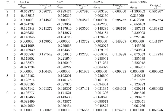
TABLE 5 Coecients ofdr:mof order statisticsXr:m inˆσm=
m ∑
r=1
dr:mXr:mandσ−2V ar(ˆσm)
m r a=1.5 a=2 a=2.5 a=4.68085
dr:m
V ar( ˆµm)
σ2 dr:m
V ar( ˆµm)
σ2 dr:m
V ar( ˆµm)
σ2 dr:m
V ar( ˆµm)
σ2
2 1 -0.658372 0.620773 -0.789474 0.607870 -0.903196 0.600060 -1.290462 0.585807
3 1 -0.438915 -0.526316 -0.602130 0.313960
2 0.000000 0.314829 0.000000 0.304842 0.000000 0.298752 0.372080 0.287523
4 1 -0.324797 -0.393037 -0.452230 -0.653163
2 -0.125548 0.211272 -0.137649 0.203520 -0.148289 0.198740 -0.187233 0.189812
5 1 -0.256351 -0.312977 -0.362187 -0.529005
2 -0.148843 -0.164723 -0.178453 -0.227546
3 0.000000 0.159056 0.000000 0.152768 0.000000 0.148865 0.000000 0.141497
6 1 -0.211068 -0.259663 -0.302027 -0.445659
2 -0.146939 -0.164360 -0.179152 -0.230894
3 -0.050587 0.127549 -0.054815 0.122280 -0.058720 0.118988 -0.073633 0.112734
7 1 -0.179002 -0.221650 -0.258961 -0.385639
2 -0.138274 -0.156219 -0.171267 -0.222948
3 -0.071794 -0.078227 -0.084079 -0.105961
4 0.000000 0.106469 0.000000 0.101939 0.000000 0.099095 0.000000 0.093662
8 1 -0.155162 -0.193201 -0.226600 -0.340242
2 -0.128214 -0.146176 -0.161119 -0.211662
3 -0.080165 -0.087923 -0.094861 -0.120283
4 -0.027142 0.091372 -0.029307 0.087401 -0.031335 0.084902 -0.039234 0.080092
9 1 -0.136777 -0.171521 -0.201396 -0.304676
2 -0.118466 -0.143400 -0.150820 -0.199707
3 -0.082499 -0.072875 -0.098671 -0.126051
4 -0.042050 -0.056454 -0.048827 -0.061266
Estimation of parameters of type-III generalized 301 wherec1:m, c2:m, . . . , cm:mandd1:m, d2:m, . . . , dm:mare constants. Now from Thomas
and Sreekumar(2008) for a random sample of size n(n > m)drawn from (1) the U-statistic for estimatingµusing the kernel(12)is given by
U1:(mn)=(1n
m )
n ∑
r=1
[m−1 ∑
i=0
( n−r m−1−i
)( r−1
i )
ci+1:m ]
Xr:n (14)
and the U-statistic for estimatingσusing the kernel (13) is given by
U2:(mn)= (1n
m )
n ∑
r=1
[m−1 ∑
i=0
( n−r m−1−i
)( r−1
i )
di+1:m ]
Xr:n, (15)
where we dene(r−1 i
)
= 0 fori≥rand(mn−−1r−i)= 0forn−r < m−1−i.
If we write
ξc(m)=Cov[h1(X1,· · ·, Xc, Xc+1,· · ·, Xm), h1(X1,· · ·, Xc, Xm+1,· · ·, X2m−c)], as the co-variance between two h1(.) functions with exactly c common
observa-tions and
ψc(m)=Cov[h2(X1,· · ·, Xc, Xc+1,· · ·, Xm), h2(X1,· · ·, Xc, Xm+1,· · ·, X2m−c)],
as the co-variance between two h2(.) functions with exactly c common
observa-tions forc= 1,2,· · · , m,then the variances ofU1:(mn) andU2:(mn) are given by (See,
Hoeding, 1948)
V ar[U1:(mn)] = (1n
m )
m ∑
c=1
( m
c )(
n−m m−c )
ξ(cm), (16)
V ar[U2:(mn)] = (1n
m )
m ∑
c=1
( m
c )(
n−m m−c )
ψc(m). (17)
Clearly
ξ(mm)=V ar[h1(X1, X2,· · ·, Xm)] (18)
and
ψm(m)=V ar[h2(X1, X2,· · · , Xm)]. (19)
It may be noted thatξm(m)andψm(m)can be obtained from tables 4 and 5 asV ar(ˆµ)
andV ar(ˆσ)respectively for m=2(1)9, a=1.5(0.5)2.5 and for a=4.68085. Now we evaluate the values ofξc(m)andψc(m)forc= 1.2, . . . , m−1, using the methodology
302 P. Yageen Thomas and R.S. Priya Dene the vectorsbm+k fork= 1,2,· · ·, m−1 as
b′m+k=
m∑−1
i=0
(
m+k−1
m−1−i )(
o i )
ci+1:m (m+k
m
) ,
m∑−1
i=0
(
m+k−2
m−1−i )(
1
i )
ci+1:m (m+k
m
) ,
· · · , m∑−1
i=0
(
0
m−1−i )(
m+k−1
i )
ci+1:m (m+k
m ) (20)
and denewk = (m+k
m )
(b′m+kVm+kbm+k)σ2−ξ (m)
m , k= 1,2,· · · , m−1whereVm+k
is the variance co-variance matrix of the vector of order statistics of a random sample of size m+k arising from g0(y) and ξ
(m)
m is dened in (18). Dene the
matrix H=
0 0 . . . 0 (mm−1)(11)
0 0 . . . (mm−2)(22) (mm−1)(21)
... ... . . . ... ...
(m 1
)(m−1 m−1
) (m 2
)(m−1 m−2
)
. . . (mm−2)(m2−1) (mm−1)(m1−1) ×
ξ(1m)
ξ(2m)
...
ξm(m−)1 (21)
and the vectorw= (w1, w2,· · ·, wm−1)′.
Then the componentsξ(cm),c= 1,2,· · · , m−1involved in (16)are solved from the
following equations (
ξ1(m), ξ2(m), . . . , ξm(m−)1 )′
=H−1W. (22)
Similarly, the values ofψ(cm),c= 1,2,· · · , m−1can be obtained as (
ψ1(m), ψ2(m), . . . , ψ(mm−)1 )′
=H−1Z, (23)
where Z′ = (z1, z2, . . . , zm−1) with zk = (m+k
m )
(gm′ +kVm+kgm+k)σ2−ψ (m)
m and
gm+k is obtained from (20) just by replacing each ci:m by di:m, i = 1,2, . . . , m.
Once we obtain the values of ξc(m), ψ (m)
c , c = 1,2, . . . , m−1 from (22) and (23)
respectively, then the exact variances of U- statistics for estimatingµandσbased
on any sample of size n can be obtained using (16) and (17) without any further direct evaluation of moments of order statistics.
Estimation of parameters of type-III generalized 303 TABLE 6
Value ofξc(m) for m=2(1)5 andc= 1,2,· · ·, m.
m c a=1.5 a=2 a=2.5 a=4.68085
2 1 0.467401 0.322469 0.245179 0.119034 2 0.934802 0.644934 0.490358 0.238068 3 1 0.203680 0.141683 0.108160 0.052791 2 0.408140 0.283670 0.216471 0.105605 3 0.616359 0.427210 0.325555 0.158526 4 1 0.113345 0.079172 0.060577 0.029649 2 0.227260 0.158578 0.121264 0.059330 3 0.342220 0.238427 0.182776 0.089034 4 0.458785 0.318953 0.243434 0.118790 5 1 0.072265 0.039859 0.038726 0.018974 2 0.144524 0.101110 0.077412 0.037941 3 0.217430 0.151901 0.116236 0.056927 4 0.290908 0.202970 0.155202 0.075937 5 0.365116 0.254346 0.194330 0.094969
U2:(mn)for any sample size, however large it may be. For example if for a given values
ofawe useµˆandˆσas given in (11) for m=4, then with the evaluation of moments
of order statistics arising from the standard Type III GLD for sample sizes up to 7, one can obtain the explicit form of appropriate U-statistic estimators forµand σ and their variances for any sample of size n, however large it may be. Using
the values of variances and co-variances of order statistics, and the coecients of BLUEs ofµandσgiven in section 3, we have obtained the values ofξc(m)andψc(m)
forc= 1,2, . . . , m−1, m=2,3,4,5 a=1.5(0.5)2.5 and for a=4.68085 and are given in table 6 and table 7. For practising statisticians these tables will be helpful to determine the variance of the U-statistics estimators.
It is unrealistic to assume always that the shape parameterainvolved in Type
III GLD is known. It is known from Balakrishnan and Lee (1998, p.130) that for a Type III GLD random variable X with pdf (1)
β2 =
E(X−µ)4
(V ar(X))2,
= 3 + ψ ′′′(a)
2(ψ′(a))2, (24)
where ψ(a)is the well known digammma function,ψ′(a)andψ′′′(a)are the rst and third derivatives of ψwith respect toa. Since the expression forβ2 as given
in(24) is free of the location parameterµ and scale parameter σ of the Type III
GLD, using a sampleX1, X2,· · · , Xndrawn from (1) we estimateaas the solution
of
3 + ψ ′′′(a) 2(ψ′(a))2 =
n ∑ i=1
(Xi−Xn)4
(
n ∑ i=1
(Xi−Xn)2)2
304 P. Yageen Thomas and R.S. Priya TABLE 7
Value ofψ(cm) for m=2(1)5 and c= 1,2,· · ·, m.
m c a=1.5 a=2 a=2.5 a=4.68085
2 1 0.161857 0.153328 0.148126 0.138381 2 0.620773 0.607870 0.600060 0.585807 3 1 0.071950 0.068145 0.065821 0.061508 2 0.176880 0.169759 0.165404 0.157344 3 0.314829 0.304842 0.298752 0.287523 4 1 0.040450 0.038324 0.037020 0.034552 2 0.089100 0.085023 0.082489 0.077730 3 0.146046 0.140085 0.136395 0.129455 4 0.211272 0.203520 0.198740 0.189812 5 1 0.025785 0.023838 0.023631 0.021945 2 0.054689 0.052070 0.050424 0.047229 3 0.086489 0.082626 0.080208 0.075680 4 0.121260 0.116180 0.113015 0.106941 5 0.159056 0.152768 0.148865 0.141497
TABLE 8
U-statistics estimates and K-S statistics for single carbon bres data set of 10mm Type III
genera-lised logistic
distribution Kernel sizes
m=2 m=3 m=4 m=5
U-statistics U1:63(2) = 3.00241 U1:63(3) = 3.00043 U1:63(4) = 2.998937 U1:63(5) = 2.98915 U2:63(2) = 0.80785 U2:63(3) = 0.80785 U2:63(4) = 0.808316 U2:63(5) = 0.78255
K-S Statistics 0.091401 0.090196 0.089172 0.089512
One may use Mathematica software for obtaining the solutionˆˆaofafrom(25). Since for the real data set describing the gauge length of single bres 10 mm considered in section 1, Type III GLD provides the best t, we once again use the data set to illustrate the U- statistics estimation of the location and scale parameters of the distribution. For the data we have computed the sample kurtosis
as n
∑
i=1
(Xi−Xn)4
(
n ∑
i=1
(Xi−Xn)2)2
= 3.234852.
On using this value in the right sidee of (25) and solving forausing mathematica
software we obtainˆˆa= 4.68085. Thus by taking 4.68085 as the known value of the parameter a we have used the method explained in this paper to obtain
U-statistics estimators U1:63(2), U1:63(3), U1:63(4), U1:63(5) for µ and U2:63(2) = U2:63(3), U2:63(4) , U2:63(5)
forσtogether with K-S statistic values and are given in table 8.
Estimation of parameters of type-III generalized 305 5. Relation Between U-Statistics Estimators and Other Standard
Estimators
Though, the U-statistics estimators developed by Thomas and Sreekumaar (2004, 2008) seems to be independent of other known estimators, their estimators for some choices of m turns out to be the same of some already known standard estimators like unbiased estimators of σbased on Gini's mean dierence and the
unbiased estimator of µ namely the sample mean X. Further we observe that U2:(2)n = U2:(3)n. In this section we discuss about these inter relationship between
U-statistics and with some other estimators.
IfX1 and X2 are two independent observations drawn from the distribution
with pdf g(x;a, µ, σ), thenYi = Xi−σµ, i=1,2 are distributed as two independent
and identically distributed random variables arising fromg0(y). Clearly
∆F =E|X1−X2|=σE(Y2:2−Y1:2) =σ(α2:2−α1:2), (26)
is dened as the Gini's mean dierence of the Type III GLD. Then an unbiased estimate of σbased on the Gini's mean dierence of the sample is given by,(see
Samuel and Thomas (2003))
σ∗= 2
n(n−1)(α2:2−α1:2) [∑n/2]
i=1
(n−2i+ 1)Ri:n, (27)
whereRi:n=Xn−i+1:n−Xi:nand [.] represents the usual greatest integer function.
Clearly σ∗ is an unbiased estimator of σ. Now we prove the following theorem
which describes the inter relationship betweenσ∗,U2:(2)nandU2:(3)nand that between Xn andU
(2) 1:n
Theorem 2. LetX1:n, X2:n, . . . , Xn;n be the order statistics of a random
sam-ple of size n arising from an absolutely continuous distribution having pdfg(x;a, µ, σ) (as dened in (1)) with location parameter µ, scale parameter σ and for given
value of the shape parameter a. Then U2:(2)n =σ∗ where σ∗ is as dened in (27).
As g(x;a, µ, σ)is symmetric about µ, we haveU2:(2)n =U2:(3)n andU1:(2)n=Xn, where Xn is the sample mean.
Proof. Using (10), one can derive the BLUEσˆ based on order statistics of a random sample of size 2 drawn fromg(x;a, µ, σ)as
ˆ
σ2= (α2:2−α1:2)−1R1:2, (28)
which is same as the kernel used for constructing the U-statistic (27). This proves that U2:(2)n =σ∗. Sinceg(x;a, µ, σ)is symmetric aboutµ, its standard formg0(y)
is symmetric about zero, and hence from (28) we further have ˆ
σ2= (2α2:2)−1R1:2. (29)
Also using the symmetric property of g(x;a, µ, σ) and using (10) for n=3 and simplifying we get
ˆ
306 P. Yageen Thomas and R.S. Priya Usingσˆ2= (2α2:2)−1R1:2 as the kernel we obtain
U2:(2)n = −1 2α2:2
(n 2
) n ∑
i=1
(n−2i+ 1)Xi:n. (31)
Ifσˆ3= (2α3:3)−1R1:3 is used as a kernel of degree 3 we obtain,
U2:(3)n = −1 2α3:3
(n
3
) n ∑
i=1
[( n−r
2
) −
( r−1
2
)] Xi:n
= −1
4α3:3
(n 3
) n ∑
i=1
[(n−2)(n−2i+ 1)]Xi:n
= −3
2α3:3n(n−1) n ∑
i=1
(n−2i+ 1)Xi:n
= 3α2:2 2α2:2
U2:(2)n. (32)
From David and Nagaraga (2003, p.49), we have
3α2:2= 2α3:3. (33)
Using the above relation in (32), we getU2:(2)n=U2:(3)n.
Using (9), and using the symmetric property ofg0(y)we can obtain the BLUE
µbased on random sample of size 2 as
ˆ
µ2= 0.5(X1:2+X2:2) =X2. (34)
Hence the corresponding U-statistic generated fromX2 is
U1:(2)n = 1
n n ∑
r=1
Xr:n =Xn (35)
and thus the theorem is proved.
6. Comparison of the U-statistic Estimators with Some Standard Un-biased Estimators
To compare the eciency of our U-statistic estimator for µ, we take the usual
moment estimatorXn ofµ, given byXn = n1 n ∑ i=1
Xi:n. ClearlyXn is the sample
mean and is unbiased forµ.
To compare the eciency of U-statistic estimator forσ, we take an unbiased
estimator ofσbased on Gini's mean dierence namelyσ∗ given in (27). In order
to compare the eciency of the U-statistic estimator of U2:(4)n and U2:(5)n with σ∗,
Estimation of parameters of type-III generalized 307 variables with common pdf (1), then considering σ∗ as a U- Statistic estimator
based on kernel of degree 2, from theorem 5.1 we have
V ar(U2:(2)n) = 2(n−2)ψ
(2) 1 +ψ
(2) 2
(n
2
) , (36)
Using (10) and (23) for m=2 and simplifying we obtain
ψ(2)1 =
[
(v1,1:3−v1,3:3)
3α2 1:2
−(v1,1:2−v1,2:2)
4α2 1:2
]
σ2and ψ2(2)=
[
(v1,1:2−v1,2:2)
2α2 1:2
]
σ2. (37) From(36) and (37), we obtain the variance of the unbiased estimatorσ∗(=U2:(2)n) as
V ar(σ∗) =(1n
2
) [
2(n−2)(v1,1:3−v1,3:3)
3α2 1:2
−(n−3)(v1,1:2−v1,2:2)
2α2 1:2
]
σ2. (38) Using the values of ξ(cm) and ψ(cm) given in table 6 and 7, we have obtained
the variances of U1:(mn) and U2:(mn) for n=5 (5) 20 (10) 40 (20) 100; m=2(1)5,
a=1.5(0.5)2.5 and for a=4.68085 and are given tables 11 and 9. In theorem 5.1, we have V ar(U1:(2)n) = V ar(Xn) and V ar(U
(2)
2:n) = V ar(U (3)
2:n) = V ar(σ∗), and hence
in table 11 and table 9 we have given the values ofV ar(Xn)instead ofV ar(U (2) 1:n)
and given the values ofV ar(σ∗)instead ofV ar(U2:(2)n)orV ar(U2:(3)n).
From tables we observe that the variances of all U-statistics reduces drastically as the sample size n increases. We also observe that the variance of U-statistics decrease as the shape parameter a of Type III GLD increases. Tandem to this
we observe that as the shape parameter a of the Type III GLD increases the
distribution tends to be one with relatively shorter tail.
For comparing the estimators inU1:(mn), we have computed the eciencye (
U1:(mn)|Xn )
ofU1:(mn) relative toXn=U (2)
1:n for m=3(1)5 and n=5( 5) 20 (10) 40 (20) 100 and
are given in table 11. It is observed that e (
U1:(mn)|Xn )
is greater than unity in all cases for m=3,4,5. For comparing the estimators in U2:(mn) we have computed
the eciencye (
U2:(mn)|σ∗ )
ofU2:(mn) relative to σ∗ =U2:(2)n =U2:(3)n is calculated for
m=4(1)5 and n=5(5) 20 (10) 40 (20) 100 and are given in table 9. It is observed thate
(
U2:(mn)|σ∗ )
is also greater than unity in all cases for m=4,5. The asymptotic relative eciencyE1,m
(
U1:(mn)|Xn )
ofU1:(mn)relative to Xn = U1:(2)n andE2,m
(
U2:(mn)|σ∗ )
ofU2:(mn)relative to σ∗=U2:(2)n =U2:(3)n are given by
E1,m (
U1:(mn)|Xn )
= lim
n→∞ [
V ar(Xn)
V ar(U1:(mn))
]
= 4ξ
(2) 1
m2ξ(m) 1
and
E2,m (
U2:(mn)|σ∗ )
= lim
n→∞ [
V ar(σ∗)
V ar(U2:(mn))
]
= 4ψ
(2) 1
m2ψ(m) 1
.
308 P. Yageen Thomas and R.S. Priya
TABLE 9 Variances ofU2:(mn) and relative eciency fore
(
U2:(mn)/σ∗ )
for m=4(1)5.
a n V ar(σ∗)
σ2
V ar(U(4)2:n)
σ2
V ar(U2:(5)n)
σ2 e
(
U2:(4)n/σ∗) e(U2:(5)n/σ∗)
1.5 5 0.159191 0.159091 0.159056 1.00070 1.00085 10 0.071344 0.071292 0.071242 1.00073 1.00143 15 0.045991 0.045961 0.045902 1.00065 1.00194 20 0.033935 0.033915 0.033855 1.00059 1.00236 30 0.022264 0.022252 0.022199 1.00054 1.00293 40 0.016567 0.016559 0.016513 1.00048 1.00327 60 0.010958 0.010953 0.010919 1.00046 1.00357 80 0.008187 0.008183 0.008156 1.00049 1.00380 100 0.006534 0.006532 0.006510 1.00031 1.00369 2 5 0.152784 0.152773 0.152768 1.00007 1.00010 10 0.068025 0.068020 0.067948 1.00007 1.00113 15 0.043756 0.043756 0.043509 1.00007 1.00568 20 0.032251 0.032251 0.031942 1.00008 1.00967 30 0.021136 0.021134 0.020827 1.00009 1.01484 40 0.015719 0.015717 0.015442 1.00013 1.01794 60 0.010392 0.010390 0.010175 1.00019 1.02133 80 0.007762 0.007760 0.007586 1.00026 1.02320 100 0.006194 0.006190 0.006048 1.00065 1.02414 2.5 5 0.148882 0.148864 0.148865 1.00012 1.00011 10 0.066002 0.065990 0.065985 1.00018 1.00026 15 0.042394 0.042384 0.042362 1.00024 1.00076 20 0.031224 0.031217 0.031189 1.00022 1.00112 30 0.020449 0.020443 0.020415 1.00029 1.00167 40 0.015202 0.015198 0.015173 1.00029 1.00191 60 0.010047 0.010044 0.010024 1.00030 1.00229 80 0.007502 0.007500 0.007485 1.00030 1.00227 100 0.005986 0.005984 0.005972 1.00033 1.00234 4.68085 5 0.141609 0.141530 0.141497 1.00056 1.00079 10 0.062220 0.062170 0.062121 1.00080 1.00159 15 0.039845 0.039810 0.039714 1.00088 1.00330 20 0.029303 0.029270 0.029173 1.00113 1.00446 30 0.019161 0.019140 0.019051 1.00110 1.00577 40 0.014234 0.014220 0.014142 1.00098 1.00651 60 0.009400 0.009390 0.009332 1.00106 1.00729 80 0.007017 0.007010 0.006963 1.00100 1.00776 100 0.005598 0.005590 0.005554 1.00143 1.00792
TABLE 10 Asymptotic relative eciencyU1:(mn) andU
(m)
2:n as estimators ofµandσ
a 1.5 2 2.5 4.68085
E1,3
(
U1:(3)n|Xn )
1.019903 1.01155 1.00747 1.002141
E1,4
(
U1:(4)n|Xn )
1.030925 1.01825 1.01185 1.003693
E1,5
(
U1:(5)n|Xn )
1.03486 1.29444 1.01298 1.003765
E2,4
( U2:(4)n|σ∗
)
1.00035 1.00021 1.00031 1.001252
E2,5
( U2:(5)n|σ∗
)
Estimation
of
par
ameters
of
typ
e-III
gener
alize
d
309
TABLE 11 Variances ofU1:(mn) and relative eciency fore
(
U1:(mn)/Xn )
for m=3(1)5
a n V ar(Xn)
σ2
V ar(U1:(3)n)
σ2
V ar(U(4)1:n)
σ2
V ar(U1:(5)n)
σ2 e
(
U1:(3)n/Xn )
e(U1:(4)n/Xn )
e(U1:(5)n/Xn )
310 P. Yageen Thomas and R.S. Priya 7. Conclusion
Thus we conclude that when a better suitable model than the well-known symmet-ric models such as: normal, double exponential, Cauchy and so on is required one may search it from the Type III GLD family of distributions. Also if one chooses a Lloyds BLUE of location and scale parameters of Type III GLD with sample size m as a kernel, then with the knowledge of the means, variances and co-variances of order statistics of random sample of sizes between m and 2m-1 arising from the standard form of the distribution, one can use the results of this paper to estimate eectively the parameters and derive their variances for any sample size (say even for n=1000 or more) by U-statistics without any further direct evaluation of mo-ments of order statistics.
Acknowledgements
The authors are highly grateful to the constructive comments of the learned reviewers which lead to a considerable improvement in the present version of the paper. The rst author of the paper express his gratefulness to Kerala State Council for Science, Technology and Environment for providing Research grand in the form of KSCSTE-Emeritus Scientist Fellowship.
References
M. G. Badar, A. M. Priest (1982). Statistical aspects of ber and bundle strength in hybrid composites. In: Hayashi T, Kawata K, Umekawa, S. (Eds.), Progress in Science and Engineering Composites. ICCM-IV, Tokyo, 1129-1136.
N. Balakrishnan (Ed) (1992). Handbook of the Logistic Distribution. Marcel Dekker, New York.
N. Balakrishnan, S. K Lee (1998). Order statistics from the Type III gener-alized logistic distribution and Applications. Handbook of Statistics, Vol 17 (Eds.,Balakrishnan N, and C. R. Rao), Elsevier Science B.V, Amsterdam. N. Balakrishnan , M. Y Leung (1988). Order statistics from the Type I
generalized logistic distribution. Communications in Statistics - Simulation and Computation, vol. 17(1), 25-50.
J. Berkson(1944). Application of the logistic function to bioassay. Journal of the American Statistical Association, 39, 357-365.
H. A. David, H. N. Nagaraja (2003). Order Statistics. Third edition, John Wiley and Sons, New York.
R. R. Davidson (1980). Some properties of a family of generalized logistic dis-tribution. In Statistical Climatology, Developments in Atmosphere Sciences, 13 (Eds., S.Ikeda et al.). Elsevier, Amsterdam.
Estimation of parameters of type-III generalized 311 414-422.
W. Hoeffding (1948). A class of statistics with asymptotically normal distribu-tions. The Annals of Mathematical Statistics, 19, 293-325.
E. H. Lloyd (1952). Least-squares estimation of location and scale parameters using order statistics. Biometrika, 39: 88-95.
N. L. Johnson, S. Kotz, N. Balakrishnan (1994). Continuous Univariate Distributions. Volume I. Second edition, John Wiley and Sons, New York. N. L. Johnson, S. Kotz, N. Balakrishnan (1995). Continuous Univariate
Distributions. Volume 2. Second edition, John Wiley and Sons, New York. F. R. Oliver (1982). Notes on the logistic curve for human populations. Journal
of the Royal Statistical Society, series A, 145, 359-363.
R. Pearl, L. J Reed (1920). On the rate of growth of the population of the United States since 1790 and its mathematical representation. Proc. Natl. Acad. Sci. 6, 275-288.
R. L. Pearl, L. J Reed (1924). Studies in Human Biology. Williams and Wilkins, Baltimore.
P. Samuel, P. Y. Thomas (2003). Estimation of parameters of triangular dis-tribution by order statistics. Calcutta Statistical Association Bulletin, 54, 45-55.
H. Schultz (1930). The standard error of a forecast from a curve. Journal of the American Statistical Association, 25, 139-185.
P. K. Sen (1990). Breakthrough in Statistics, Vol-I. Edited by Kotz, S and John-son, N. L., Springer, NewYork.
N. V Sreekumar, P. Y. Thomas (2006). Estimation of the scale parameters of linear exponential distribution using order statistics. IAPQR Translations,Vol-31,No.2, 99-112.
N. V Sreekumar, P. Y. Thomas (2007). Estimation of the parameters of log-gamma distribution using order statistics. Metrika, vol.66, no. 1, 115-127. N. V Sreekumar, P. Y. Thomas (2008). Estimation of the parameters of
Type-I generalized logistic distribution using order statistics. Communications in Statistics-theory and Methods, vol. 37,no.10, 1506-1524.
P. Y. Thomas (1990). Estimating location and scale parameters of a symmetric distribution by systematic statistics. Journal of the Indian Society of Agricul-tural Statistics, 42: 250-256.
P. Y. Thomas, N. V. Sreekumar (2004). Estimation of the scale parameters of generalized exponential distribution using order statistics. Calcutta Statistical Association Bulletin, 55, 199-208.
P. Y. Thomas, N. V. Sreekumar (2008). Estimation of location and scale parameters of a distribution by U-statistics based on best linear functions of order statistics. Journal of Statistical Planning and Inference, 138, no. 7: 2190-2200.
Skew-312 P. Yageen Thomas and R.S. Priya normal distribution usingU-statistics on order statistics. Calcutta Statistical Association Bulletin,64, 1-20.
E.B. Wilson, J. Worcester (1943). The determination of L. D. 50 and its sampling error in bioassay. Proc. Natl. Acad. Sci. 29,79-85.
Summary
In this work we have derived appropriate U-statistics from a sample of any size exceeding a specied integer to estimate the location and scale parameters of Type III generalized logistic distribution without the knowledge or by evaluation of the means, variances and co-variances of order statistics of an equivalent sample size arising from the corresponding standard form of distribution. The exact variances and the asymptotic variances of the estimators have been obtained. The eciency of the obtained estimators relative to some of the standard estimators have been also obtained. An illustration describing the betterness of U-statistics estimation method over the classical maximum-likelihood method is also given.