House of risk: a model
for proactive supply chain
risk management
I. Nyoman Pujawan and Laudine H. Geraldin
Department of Industrial Engineering,
Sepuluh Nopember Institute of Technology, Surabaya, Indonesia
Abstract
Purpose– Increasingly, companies need to be vigilant with the risks that can harm the short-term operations as well as the long-term sustainability of their supply chain (SC). The purpose of this paper is to provide a framework to proactively manage SC risks. The framework will enable the company to select a set of risk agents to be treated and then to prioritize the proactive actions, in order to reduce the aggregate impacts of the risk events induced by those risk agents.
Design/methodology/approach– A framework called house of risk (HOR) is developed, which combines the basic ideas of two well-known tools: the house of quality of the quality function deployment and the failure mode and effect analysis. The framework consists of two deployment stages. HOR1 is used to rank each risk agent based on their aggregate risk potentials. HOR2 is intended to prioritize the proactive actions that the company should pursue to maximize the cost-effectiveness of the effort in dealing with the selected risk agents in HOR1. For illustrative purposes, a case study is presented. Findings– The paper shows that the innovative model presented here is simple but useful to use. Research limitations/implications– In the proposed framework, the correlations between risk events are ignored, something that future studies should consider including.
Practical implications– The framework is intended to be useful in practice. For the calculation processes, a simple spreadsheet application would be sufficient. However, most of the entries needed in the model are based on subjective judgment and hence cross-functional involvement is needed. Originality/value– The paper adds to the SC management literature, a novel practical approach of managing SC risks, in particular to select a set of proactive actions deemed cost-effective.
KeywordsSupply chain management, Risk management Paper typeResearch paper
Introduction
Business communities are facing increasingly more risky environments recently. Stringent competitions, internal instability caused by employee strikes and technical failures, changes in macro-economy and politics, as well as natural and man-made disasters are sources of risks facing business communities nowadays. In the context of supply chain (SC), the increasing risks are partly due network complexity as a result of companies outsourcing more activities to outside parties. A study conducted by Finch (2004) revealed that the inter-organizational networking increased large companies’ exposure to risks, especially if the partners are small and medium enterprises. Craighead
et al.(2007) argues that SC structure which includes such factors as density, complexity, and node criticality could increase the severity of SC disruptions. In addition, factors such as reduction of supply base, globalization of SC, shortened product life cycles, and capacity limitation of key components also increase SC risks (Norrman and Jansson, 2004).
The current issue and full text archive of this journal is available at
www.emeraldinsight.com/1463-7154.htm
Supply chain
risk management
953
Business Process Management Journal Vol. 15 No. 6, 2009 pp. 953-967
qEmerald Group Publishing Limited 1463-7154 DOI 10.1108/14637150911003801
Risk is a function of the level of uncertainty and the impact of an event (Sinhaet al.,
2004). As pointed out by Gohet al.(2007) there are two types of SC risks based on their
sources: risks arising from the internal of the SC network and those from the external environments. Tang (2006a) classified SC risks into operations and disruptions risks. The operations risks are associated with uncertainties inherent in a SC which include demand, supply, and cost uncertainties. Disruption risks, on the other hand, are those caused by major natural and man-made disasters such as flood, earthquake, tsunami, and major economic crisis. Both operations and disruption risks could seriously disrupt and delay materials, information, and cash flow, which in the end could damage sales, increase costs, or both (Chopra and Sodhi, 2004). Analysis conducted by Hendricks and Singhal (2003, 2005) show that companies experiencing disruption risks were significantly outperformed by their peers in terms of operating as well as stock performance.
To survive in a risky business environment, it is imperative for companies to have a proper SC risk management. If poorly handled, disruptions in SC could result in costly
delays causing poor service level and high cost (Blackhurstet al., 2005). According to
Norrman and Jansson (2004), the focus of SC risk management is to understand, and try to avoid, the devastating effects that disasters or even minor business disruptions can have in a SC. The aim of SC risk management is to reduce the probability of risk events occurring and to increase resilience, that is, the capability to recover from a disruption. Sheffi and Rice (2005) suggest that the SC resilience can be improved by either creating redundancy or improving flexibility. However, as suggested by Ritchie and Brindley (2007), classic SC risk management such as maintaining buffer stocks and slack lead times are becoming less viable nowadays. With the increasing interest in SC management, where companies no longer focus solely on their own organizations, the SC risk management should also be managed in relation with inter-organizational view. Risk in the SC centers around the major flows (materials, information, and cash) between organizations and hence, SC risks extend beyond the boundaries of a single firm ( Juttner, 2005).
In this paper, we present an innovative model for proactive SC risk management. The term proactive is used to imply preventive nature of the effort in the sense that we mostly deal with the risk agents. This is based on the notion that attacking the causes (or the risk agents) could concurrently prevent one or more risk events from happening. We modified the well-known failure mode and effect analysis (FMEA) model for risk quantification and adapt the house of quality (HOQ) model for prioritizing which risk agents are to be dealt with first and for selecting the most effective actions in order to reduce the risks potentially posed by the risk agents. In the quantification stage, we first define basic SC processes based on the supply chain operations reference (SCOR) terminology. The core SC processes will be analyzed to identify the risks that could happen and the consequences if it happened. The risk agents and their associated probabilities are also assessed. We defined aggregate risk potential for each risk agent as the aggregate severity of impacts caused by a risk agent. To provide an illustration on how the model works, we present the application of the model to a large fertilizer company in Indonesia.
Existing models for SC risk assessment and mitigation
Assessing the risk level related to SC under which an organization is operating is a crucial step in SC risk management (Kull and Closs, 2008). A number of different models
BPMJ
15,6
for risk assessment and mitigation have been proposed in the literature. Sinhaet al.
(2004) proposed a methodology to mitigate SC risks. The model involves the process of identifying, assessing, planning and implementing solution, conducting FMEA analysis, and doing continuous improvement. The five activities were modeled in IDEF0 where each activity should have an input, an output, a mechanism, and a control. The model was applied to a supplier in the aerospace industry. In the FMEA stage, the risk potential number (RPN) of each potential failure mode is a product of the probability
of a failure mode occurring (P) and the associated severity of impacts generated (S) if it
occurred. Both thePandSwere assessed subjectively using a scale of 1-10.
A SC risk management model for Ericsson, a leading telecom company based in Sweden, was proposed by Norrman and Jansson (2004). The model was developed in the form of a closed-loop process of risk identification, risk assessment, risk treatment, and risk control. In parallel to these processes, the model also includes incident handling and contingency planning.
Kleindorfer and Saad (2005) proposed a methodology in dealing with SC disruption risks. The methodology includes three general processes, called specifying resources of risk and vulnerabilities, assessment, and mitigation. To implement the above-three tasks, the authors proposed ten principles derived from industrial risk and SC management literatures.
Cucchiella and Gastaldi (2006) presented a real option approach for managing SC
risks. The proposed model include six steps (Harlandet al., 2003) to be carried out:
analysis of SC, identify uncertainty sources, examine the subsequent risk, manage risk, individualize the most adequate real option, and implement SC risk strategy. The real option types considered in the paper include defer, stage, explore, lease, outsource, scale down, scale up, abandon switch, and strategic grow.
Analytical hierarchy process (AHP) has also been used to assess risk in a SC (Gaudenzi and Borghesi, 2006). The AHP was used to prioritize SC objectives, identifying risk indicators, as well as assessing the potential impact of negative events and the cause-effects relationships along the chain. The authors suggest that SC risk management can be considered as a process that supports the achievement of SC management objectives.
House of risk model
Our model is based on the notion that a proactive SC risk management should attempt to focus on preventive actions, i.e. reducing the probability of risk agents to occur. Reducing occurrence of the risk agents would typically prevent some of the risk events to occur. In such a case, it is necessary to identify the risk events and the associated risk agents. Typically, one risk agent could induce more than one risk events. For example, problems in a supplier production system could result in shortage of materials and increased reject rate where the latter is due to switching procurement to other, less capable, suppliers.
In the well-known FMEA, risk assessment is done through calculation of a RPN as a product of three factors, i.e. probability of occurrence, severity of impacts, and detection. Unlike in the FMEA model where both the probability of occurrence and the degree of severity are associated with the risk events, here we assign the probability to the risk agent and the severity to the risk event. Since one risk agent could induce a number of risk events, it is necessary to quantity the aggregate risk potential of a risk
Supply chain
risk management
agent. IfOjis the probability of occurrence of risk agentj,Siis the severity of impact if
risk eventioccurred, andRijis the correlation between risk agentjand risk eventi
(which is interpreted as how likely risk agentjwould induce risk eventi) then the ARPj
(aggregate risk potential of risk agentj) can be calculated as follows:
ARPj¼Oj
i
X
SiRij ð1Þ
We adapt the HOQ model to determine which risk agents should be given priority for preventive actions. A rank is assigned to each risk agent based on the magnitude of the
ARPjvalues for eachj. Hence, if there are many risk agents, the company can select first a
few of those considered having large potentials to induce risk events. In this paper, we propose two deployment models, called HOR, both of which are based on the modified HOQ: (1) HOR1 is used to determine which risk agents are to be given priority for
preventive actions.
(2) HOR2 is to give priority to those actions considered effective but with reasonable money and resource commitments.
HOR1
In the HOQ model, we relate a set of requirements (what) and a set of responses (how) where each response could address one or more requirements. The degree of correlation is typically classified as none (and given an equivalent value of 0), low (one), moderate (three), and high (nine). Each requirement has a certain gap to fill and each response would require some types of resources and funds.
Adopting the above procedure, the HOR1 is developed through the following steps: (1) Identify risk events that could happen in each business process. This can be done through mapping SC processes (such as plan, source, deliver, make, and return) and then identify “what can go wrong” in each of those processes.
Ackermannet al.(2007) provide a systematic way of identifying and assessing
risks. In HOR1 model shown in Table I, the risk events are put in the left
column, represented asEi.
Risk
event Risk agents (Aj)
Severity of risk event Business processes (Ei) A1 A2 A3 A4 A5 A6 A7 i(Si) Plan E1 R11 R12 R13 S1 E2 R21 R22 S2 Source E3 R31 S3 E4 R41 S4 Make E5 S5 E6 S6 Deliver E7 S7 E8 S8 Return E9 S9 Occurrence of agentj O1 O2 O3 O4 O5 O6 O7 Aggregate risk potentialj ARP1 ARP2 ARP3 ARP4 ARP5 ARP6 ARP7 Priority rank of agentj
Table I. HOR1 model
BPMJ
15,6
(2) Assess the impact (severity) of such risk event (if happened). We use a 1-10 scale where 10 represents extremely severe or catastrophic impact (see Shahin (2004) for a detailed verbal description about the scale). The severity of each risk event is
put in the right column of Table I, indicated asSi.
(3) Identify risk agents and assess the likelihood of occurrence of each risk agent. Here, a scale of 1-10 is also applied where 1 means almost never occurred and a value of
10 means almost certain to happen. The risk agents (Aj) are placed on top row of the
table and the associated occurrence is on the bottom row, notated asOj.
(4) Develop a relationship matrix, i.e. relationship between each risk agent and
each risk event,Rij{0, 1, 3, 9} where 0 represents no correlation and 1, 3, and 9
represent, respectively, low, moderate, and high correlations.
(5) Calculate the aggregate risk potential of agentj(ARPj) which is determined as the
product of the likelihood of occurrence of the risk agentjand the aggregate impacts
generated by the risk events caused by the risk agentjas in equation (1) above.
(6) Rank risk agents according to their aggregate risk potentials in a descending order (from large to low values).
HOR2
HOR2 is used to determine which actions are to be done first, considering their differing effectiveness as well as resources involved and the degree of difficulties in performing. The company should ideally select set of actions that are not so difficult to perform but could effectively reduce the probability of risk agents occurring.
The steps are as follows:
(1) Select a number of risk agents with high-priority rank, possibly using Pareto
analysis of the ARPj, to be dealt with in the second HOR. Those selected will be
placed in the left side (what) of HOR2 as depicted in Table II. Put the
corresponding ARPjvalues in the right column.
(2) Identify actions considered relevant for preventing the risk agents. Note that one risk agent could be tackled with more than one actions and one action could simultaneously reduce the likelihood of occurrence of more than one risk agent. The actions are put on the top row as the “How” for this HOR.
Preventive action (PAk) Aggregate risk potentials To be treated risk agent (Aj) PA1 PA2 PA3 PA4 PA5 (ARPj)
A1 E11 ARP1
A2 ARP2
A3 ARP3
A4 ARP4
Total effectiveness of actionk TE1 TE2 TE3 TE4 TE5 Degree of difficulty performing
actionk D1 D2 D3 D4 D5
Effectiveness to difficulty ratio ETD1 ETD2 ETD3 ETD4 ETD5
Rank of priority R1 R2 R3 R4 R5 Table II. HOR2 model
Supply chain
risk management
957
(3) Determine the relationship between each preventive action and each risk agent,
Ejk. The values could be {0, 1, 3, 9} which represents, respectively, no, low,
moderate, and high relationships between action k and agent j. This
relationship (Ejk) could be considered as the degree of effectiveness of actionkin
reducing the likelihood of occurrence of risk agentj.
(4) Calculate the total effectiveness of each action as follows:
TEk¼
j
X
ARPjEjk ;k ð2Þ
(5) Assess the degree of difficulties in performing each action,Dk, and put those
values in a row below the total effectiveness. The degree of difficulties, which can be represented by a scale (such as Likert or other scale), should reflect the fund and other resources needed in doing the action.
(6) Calculate the total effectiveness to difficulty ratio, i.e. ETDk¼TEk=Dk.
(7) Assign rank of priority to each action (Rk) where Rank 1 is given to the action
with the highest ETDk.
Case example
Brief company background
We applied the above models to a large government-owned fertilizer company in Indonesia. The company has three production plants and produces a wide range of fertilizer, including Urea, TSP, and ZA. The raw materials used in these plants include natural gas and a number of chemical substances such as sulfur and potassium chloride. The aggregate capacity of the three plants is above 3 million tons per year. The main products are distributed to all regions in Indonesia which are divided into two distribution areas. As a government-owned company, the pricing, marketing, and distribution of the products should comply with the government regulations. Although most of the information presented in this case study has been based on our field study with the company, for some reasons, some of the results have been modified by the authors.
Identification of risk events and assessment of their severity
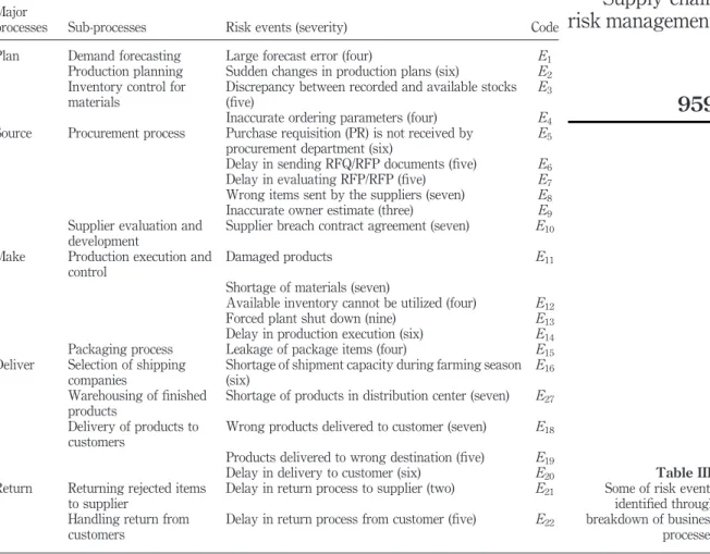
The risk events were identified through breakdown of major business processes into sub-processes and then asking the question of “what can go wrong?” in each of the sub-processes. We followed the five major SC processes according to SCOR terminologies defined by the SC council. The company has already documented risk events before this study was carried out so we included many of already defined risk events in this study. Some of other risk events were identified during the study, through interview and brainstorming with relevant managers, which then led us to have a total of 22 risk events (four of which are associated with plan, six with source, five with make, five with deliver, and two with return). Some of the identified risk events are presented in Table III.
The next step is the assessment of severity of each risk event. This was accomplished by distributing questionnaire to relevant managers. They were asked to fill in a number (between 1 and 10) next to each risk event where a value of 1 means almost no impact if the associated risk event occurred while a value of 10 means hazardous impact (see
BPMJ
15,6
Shahin (2004) for a more detailed description of the scales). Numbers in the parentheses in Table III represent the severity of the associated risk events.
Identification of risk agents
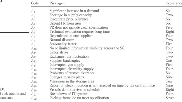
Many of the risk agents had also been documented by the company. However, we did make clarification and suggest some other possible risk agents not included in their list. Finally, we ended up with a total of 22 risk agents as presented in Table IV along with their respective degree of occurrence. The occurrence represents the probability of each of those risk agents happening. The values range from one to ten where a value of 1 means almost never occurred and a value of 10 means almost certain to happen (Shahin, 2004). The values of occurrence were also obtained through questionnaire distributed to relevant managers.
Identification of correlation between risk agents and risk events
The relationship between the risk agents and risk events were identified and a value of 0, 1, 3, or 9 was assigned in each combination. We obtain, for example, a value of Major
processes Sub-processes Risk events (severity) Code
Plan Demand forecasting Large forecast error (four) E1
Production planning Sudden changes in production plans (six) E2 Inventory control for
materials
Discrepancy between recorded and available stocks (five)
E3 Inaccurate ordering parameters (four) E4 Source Procurement process Purchase requisition (PR) is not received by
procurement department (six)
E5 Delay in sending RFQ/RFP documents (five) E6 Delay in evaluating RFP/RFP (five) E7 Wrong items sent by the suppliers (seven) E8 Inaccurate owner estimate (three) E9 Supplier evaluation and
development
Supplier breach contract agreement (seven) E10 Make Production execution and
control
Damaged products E11
Shortage of materials (seven)
Available inventory cannot be utilized (four) E12 Forced plant shut down (nine) E13 Delay in production execution (six) E14 Packaging process Leakage of package items (four) E15 Deliver Selection of shipping
companies
Shortage of shipment capacity during farming season (six)
E16 Warehousing of finished
products
Shortage of products in distribution center (seven) E27 Delivery of products to
customers
Wrong products delivered to customer (seven) E18 Products delivered to wrong destination (five) E19 Delay in delivery to customer (six) E20 Return Returning rejected items
to supplier
Delay in return process to supplier (two) E21 Handling return from
customers
Delay in return process from customer (five) E22
Table III. Some of risk events identified through breakdown of business processes
Supply chain
risk management
959
9 between A14 (interrupted gas supply) and E13 (forced plant shut down), indicating
that the interrupted gas supply would certainly result in forced plant shut down. The relationships between each risk agent and each risk event is shown in HOR1 in Table V.
Aggregate risk potentials
With the three inputs above, we can calculate the aggregate risk potentials of each risk agent. As an illustration, consider risk agent 1 (significant increase in demand). The likelihood of this agent occurring is 6 in the 1-10 scale. This risk agent has a high correlation (scored 9) with four risk events, each with degree of severity of 4, 4, 7, and 7, a moderate correlation with one risk event with an associated severity of 6, and a low correlation with an associated severity of 6. Hence, the ARP of this risk agent is calculated as follows:
ARP1¼6£½9ð4þ4þ7þ7Þ þ3ð6Þ þ1ð6Þ ¼1;332
As can be seen from Table V, the calculated values range from 56 to 1,539. The Pareto diagram of the aggregate risk potentials for all 22 risk events is shown in Figure 1. The results show that there is only one risk agent with an ARP value of more than 1,500; four risk agents with an ARP value between 1,000 and 1,500; six risk agents with an ARP value between 500 and 1,000; and the rests (11) have an ARP value below 500. Further analysis shows that the first five risk agents contribute to about 50 percent of the total ARP values and ten risk agents contribute to 75 percent of the total ARP.
Identification and prioritizing proactive actions
The above-Pareto diagram indicates that the degree of importance of reducing the probability of occurrence of each risk agent differs widely. Naturally, a company
Code Risk agent Occurrence
A1 Significant increase in a demand Six
A2 Shortage in supply capacity Two
A3 Inaccurate price reference Six
A4 Urgent PR from user Six
A5 PR does not include clear specification Five
A6 Technical evaluation requires long time Eight
A7 Dependence on one supplier Four
A8 Natural disaster Two
A9 Seasonality factor Five
A10 No or limited information visibility across the SC Four
A11 Labor strike Two
A12 Exchange rate fluctuation Two
A13 Supplier bankruptcy One
A14 Interrupted gas supply Five
A15 Interrupted electricity supply Four
A16 Problems of custom clearance Six
A17 Changes in sales plans Nine
A18 Messiness in the storage area Ten
A19 Report on stock mutation is not received on time by the central office Nine
A20 Vessels do not arrive on schedule Eight
A21 Breakdown of IT system Four
A22 Package items do no meet specification Seven
Table IV.
Some of risk agents and their occurrence
BPMJ
15,6
Risk agents Risk events A1 A2 A3 A4 A5 A6 A7 A8 A9 A10 A11 A12 A13 A14 A15 A16 A17 A18 A19 A20 A21 A22 Si E1 93 3 1 4 E2 33 1 3 6 E3 19 3 5 E4 91 1 4 E5 33 6 E6 39 9 3 1 9 5 E7 33 9 3 1 3 5 E8 9 7 E9 33 3 3 3 9 3 3 E10 97 E11 9 9 3133 33 1 3 9 1 3 4 E12 33 3 1 7 E13 93 9 1 9 9 6 E14 93 3 3 3 1 9 3 9 E15 96 E16 39 1 9 4 E17 93 1 3 9 3 3 3 1 3 9 7 E18 13 3 7 E19 13 6 E20 13 1 3 1 3 3 3 1 9 7 E21 11 1 1 7 E22 11 1 1 5 Oj 6266 5842542 2 1 54669 1 0 9 8 4 ARP j 1,332 510 126 180 1,070 776 168 320 800 560 358 56 99 1,200 396 180 426 630 870 1,539 1,032 216 Pj 2 1 1 2 0 1 7 4 8 1 9 1 5 7 10 14 22 21 3 1 3 1 8 1 2 9 6 1 5 16 Note: Ei and Aj refers to the definition in Tables III and IV, respectively Table V. HOR1 of the case company
Supply chain
risk management
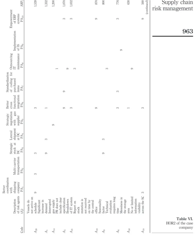
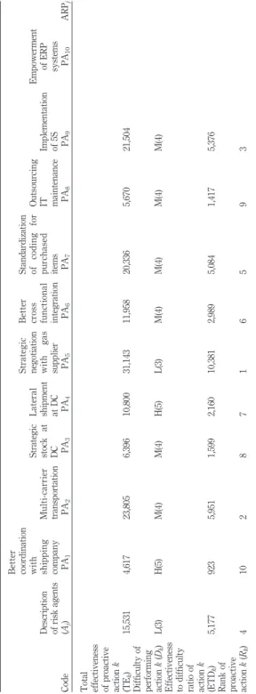
should prioritize those with high-aggregate risk potentials. For illustrative purposes, we picked the ten risk agents which contribute to about 75 percent of the total ARP. The second HOR framework in the section three can be used to identify and prioritize proactive actions that the company should do in order to maximize the effectiveness of effort with acceptable resource and financial commitments. The HOR2 which presents the ten risk agents with the ten proposed actions is depicted in Table VI. The difficulty of performing each action is classified into three categories: low with a score of 3, medium with a score of 4, and high with a score of 5. As pointed out above, the degree of difficulty should also reflect the money and other resources needed to perform the corresponding action. Hence, the ratio would indicate the cost effectiveness of each action. However, we should aware that the use of different scale in measuring the degree of difficulty may result in changes of the ranks, indicating the need to perform sensitivity analysis when applying this framework in a real case.
The priority for each action is obtained based on the values of the effectiveness to
difficulty ratio of actionk(ETDk). The higher the ratio, the more cost effective is the
proposed action. From Table VI, we see that the most cost effective action would be to improve the cross functional team within the organization.
In general, the actions could be strategic or tactical in nature. Juttneret al.(2003)
suggest that mitigation actions could be in the form of avoidance, control, cooperation, and flexibility. Risk avoidance could be done by, for example, dropping specific products/geographical markets. Risk control can be done by vertical integration and increasing the inventory buffer, while cooperation can be in the form of sharing risk information and jointly develop a contingency plan with suppliers. A number of efforts to increase flexibility, as another form of risk mitigation strategies, can be done through postponing activities deemed risky to be done before receiving orders from customers and establishing multiple suppliers. Similarly, Tang (2006b) provides a list Figure 1.
Pareto diagram of aggregate risk potentials of all risk agents 0 200 400 600 800 1,000 1,200 1,400 1,600 1,800
A20 A1 A14 A5 A21 A19 A9 A6 A18 A10 A2 A17 A15 A11 A8 A22 A4 A16 A7 A3 A13 A12
Risk agent 0.0 20.0 40.0 60.0 80.0 100.0 120.0 ARPj Cum. ARPj
BPMJ
15,6
962
Description of risk agents Be tt er coordination wi th shi pping company Multi -car rier transportation Strategic stock at DC La te ra l shipment at DC Strategic negotiation wi th g a s supplier Be tt er cross funct io n al integration Standardization of coding for purchased items Ou ts ou rc in g IT maintenance Implementation of 5S Empowerment of ERP systems Code ( Aj)P A1 PA 2 PA 3 PA 4 PA 5 PA 6 PA 7 PA 8 PA 9 PA 10 ARP j A20 Vessels do not arrive o n schedule 9 3 3 3 1,539 A1 Significant increase in demand 9 3 1 1,332 A14 Interrupted gas supply 9 1,200 A5 PR does not include clear specification 9 9 1 3 1 ,070 A21 Breakdown of IT system 3 9 3 1 ,032 A19 Report on stock mutation is not received on time b y the central office 9 3 9 870 A9 Seasonality factor 9 3 800 A6
Technical evaluation requires
long time 3 3 3 3 776 A18 Messiness in the storage area 1 9 630 A10 No or limited
information visibility across
the S C 3 3 9 9 560 ( continued ) Table VI. HOR2 of the case company
Supply chain
risk management
Description of risk agents Be tt er coordination wi th shi pping company Multi -car rier transportation Strategic stock at DC La te ra l shipment at DC Strategic negotiation wi th g a s supplier Be tt er cross funct io n al integration Standardization of coding for purchased items Ou ts ou rc in g IT maintenance Implementation of 5S Empowerment of ERP systems Code ( Aj )P A1 PA 2 PA 3 PA 4 PA 5 PA 6 PA 7 PA 8 PA 9 PA 10 ARP j Total effectiveness of proactive action k (TE k ) 15,531 4,617 23,805 6,396 10,800 31,143 11,958 20,336 5,670 21,504 Difficulty of performing action k ( Dk ) L (3) H(5) M(4) M(4) H(5) L(3) M(4) M(4) M(4) M(4) Effectiveness to difficulty ratio of action k (ETD k ) 5,177 923 5,951 1,599 2,160 10,381 2,989 5,084 1,417 5,376 Rank of proactive action k ( Rk )4 1 0 2 8 7 1 6 5 9 3 Table VI.
BPMJ
15,6
964
of possible strategies for designing a robust SC. These include postponement, strategic stock, flexible supply base, flexible transportation, and silent product rollover. Sodhi and Lee (2007) present various possible strategies to mitigating SC risk, in particular within the consumer electronic industry sector.
Discussions and concluding remarks
We presented a model for proactive risk management in this paper. We adapted the well-known HOQ model to determine which risk actions to be tackled first and to select a set of proactive actions deemed cost-effective to be prioritized. The proposed model is different from the previous models in the sense that we select the risk agents having large aggregate risk potentials, i.e. those with high probability of occurring and causing many risk events with severe impacts. In HOR2 model, we prioritize the actions based on the ratio of the total effectiveness to the degree of difficulty. Since the degree of difficulty includes such considerations as money and other resources needed, the ratio would reflect the cost effectiveness of each action.
To the best of our knowledge, the HOR model presented in this paper has never been proposed in any previous literature on SC risk management. As an illustration of the application of the model, we present a case study of a large fertilizer company in Indonesia. The model is intended to be generic in nature, so that it can be implemented to any type of companies without much changes needed. The procedure would still be the same, although the types of risk events, the risk agents, and the strategies to mitigate the risks would vary from case to case.
While the model can be easily implemented in practice, where a simple spreadsheet can be used to do the calculation needed in the two HOR models, the input to the model requires significant data collection and brainstorming within the organization. A good cross-functional team would be required to arrive at the identification and definition of the risk events and risk agents, their associated degree of severity and rate of occurrence as well as the correlation between each risk agent and each risk event. Reference to previous works in the relevant industry sector would certainly be useful in the brainstorming process.
In this paper, we ignored the dependence between risk events. In reality such dependencies could happen. For example, if there is a large forecast error, the values of the ordering parameters such as safety stock and reorder point tend to be less accurate. Likewise, delivery delay to customers would increase the chance of having a shortage at the distribution center. In future studies, such dependencies should be taken into account. The use of analytical network process in determining the relative severity of risk event could be considered as a way to handle dependencies between risk events.
References
Ackermann, F., Eden, C., Williams, T. and Howick, S. (2007), “Systematic risk assessment: a case study”,Journal of the Operational Research Society, Vol. 58 No. 1, pp. 39-51.
Blackhurst, J., Craighead, C.W., Elkins, D. and Handfield, R.B. (2005), “An empirically derived agenda of critical research issues for managing supply chain disruptions”,International Journal of Production Research, Vol. 43 No. 19, pp. 4067-81.
Chopra, S. and Sodhi, S.M. (2004), “Managing risk to avoid supply-chain breakdown”,Sloan Management Review, Vol. 46 No. 1, pp. 53-61.
Supply chain
risk management
Craighead, C.W., Blackhurst, J., Rungtusanatham, M.J. and Handfield, R.B. (2007), “The severity of supply chain disruptions: design characteristics and mitigation capabilities”,Decision Sciences, Vol. 38 No. 1, pp. 131-56.
Cucchiella, F. and Gastaldi, M. (2006), “Risk management in supply chain: a real option approach”, Journal of Manufacturing Technology Management, Vol. 17 No. 6, pp. 700-20.
Finch, P. (2004), “Supply chain risk management”,Supply Chain Management: An International Journal, Vol. 9 No. 2, pp. 183-96.
Gaudenzi, B. and Borghesi, A. (2006), “Managing risk in the supply chain using the AHP method”,The International Journal of Logistics Management, Vol. 17 No. 1, pp. 114-36. Goh, M., Lim, J.Y.S. and Meng, F. (2007), “A stochastic model for risk management in
global supply chain networks”, European Journal of Operational Research, Vol. 182, pp. 164-73.
Harland, C., Brenchley, R. and Walker, H. (2003), “Risk in supply networks”, Journal of Purchasing and Supply Management, Vol. 9 No. 2, pp. 51-62.
Hendricks, K.B. and Singhal, V.R. (2003), “The effect of supply chain glitches on shareholder wealth”,Journal of Operations Management, Vol. 21, pp. 501-22.
Hendricks, K.B. and Singhal, V.R. (2005), “An empirical analysis of the effect of supply chain disruptions on long-run stock price performance and equity risk of the firm”,Production and Operations Management, Vol. 14 No. 1, pp. 35-52.
Juttner, U. (2005), “Supply chain risk management: understanding the business requirements from a practitioner perspective”,International Journal of Logistics Management, Vol. 16 No. 1, pp. 120-41.
Juttner, U., Peck, H. and Christopher, M. (2003), “Supply chain risk management: outlining an agenda for future research”,International Journal of Logistics: Research and Application, Vol. 6 No. 4, pp. 197-210.
Kleindorfer, P.R. and Saad, G.H. (2005), “Managing disruption risks in supply chains”, Production and Operations Management, Vol. 14 No. 1, pp. 53-68.
Kull, T. and Closs, D. (2008), “The risk of second-tier supplier failures in serial supply chains: implications for order policies and distributor autonomy”, European Journal of Operational Research, Vol. 186 No. 3, pp. 1158-74.
Norrman, A. and Jansson, U. (2004), “Ericsson’s proactive supply chain risk management approach after a serious sub-supplier accident”, International Journal of Physical Distribution & Logistics Management, Vol. 34 No. 5, pp. 434-56.
Ritchie, B. and Brindley, C. (2007), “An emergent framework for supply chain risk management and performance measurement”,Journal of the Operational Research Society, Vol. 58 No. 11, pp. 1398-411.
Shahin, A. (2004), “Integration of FMEA and the Kano model: an exploratory examination”, International Journal of Quality & Reliability Management, Vol. 21 No. 7, pp. 731-46. Sheffi, Y. and Rice, J.B. Jr (2005), “A supply chain view of the resilient enterprise”,MIT Sloan
Management Review, Vol. 47 No. 1, pp. 41-8.
Sinha, P.R., Whitman, L.E. and Malzahn, D. (2004), “Methodology to mitigate supplier risk in an aerospace supply chain”,Supply Chain Management: An International Journal, Vol. 9 No. 2, pp. 154-68.
Sodhi, M.S. and Lee, S. (2007), “An analysis of sources of risk in the consumer electronics industry”,Journal of the Operational Research Society, Vol. 58 No. 11, pp. 1430-9.
BPMJ
15,6
Tang, C.S. (2006a), “Perspectives in supply chain risk management: a review”,International Journal of Production Economics, Vol. 103, pp. 451-8.
Tang, C.S. (2006b), “Robust strategies for mitigating supply chain disruptions”,International Journal of Logistics: Research and Application, Vol. 9 No. 1, pp. 33-45.
Corresponding author
I. Nyoman Pujawan can be contacted at: [email protected]
Supply chain
risk management
967
To purchase reprints of this article please e-mail:[email protected]