1
Supplementary material
Foraging ecology of the common dolphin Delphinus delphis revealed by stable isotope analysis
Katharina J. Peters*1,2, Sarah J. Bury3, Emma Betty1, Guido J. Parra4, Gabriela
Tezanos-Pinto1,5 & Karen A. Stockin1
Author affiliations:
1Cetacean Ecology Research Group, School of Natural and Computational Sciences, Massey University,
Auckland 0745, New Zealand
2Global Ecology, College of Science and Engineering, Flinders University, Adelaide 5001, South Australia
3National Institute of Water and Atmospheric Research, Greta Point, 301 Evans Bay Parade, Hataitai,
Wellington 6021, New Zealand
4Cetacean Ecology, Behaviour and Evolution Lab, College of Science and Engineering, Flinders
University, Adelaide 5001, South Australia
5Molecular Ecology of Aquatic Vertebrates Lab (LEMVA), Los Andes University, Bogota 11711,
Colombia
*Corresponding author: [email protected]
Extended methods
Details on stable isotope analysis
Carbon isotope data were corrected via a 2-point normalisation process (Paul et al. 2007) using NIST 8573 (USGS40 L-glutamic acid; certified δ13C = - 26.39 ± 0.09 ‰) and NIST
8542 (IAEA-CH-6 Sucrose; certified δ13C = - 10.45 ± 0.07 ‰). A 2-point normalisation
process using NIST 8573 (USGS40 L-glutamic acid; certified δ15N = - 4.52 ± 0.12 ‰) and
IAEA-N-2 (ammonium sulphate: certified δ15N = + 20.41 ± 0.2 ‰) was applied to δ15N data.
DL-Leucine (DL-2-Amino-4-methylpentanoic acid, C6H13NO2, Lot 127H1084, Sigma,
Australia) was run every ten samples to check analytical precision and enable drift
corrections to be made if necessary. NIST 8547 (IAEA-N1 ammonium sulphate; certified
δ15N = + 0.43 ± 0.04 ‰) and USGS65 Glycine (certified δ13C = - 20.29 ± 0.04 ‰; certified
δ15N = 20.68 ± 0.06 ‰) were run daily to check isotopic accuracy with 2 laboratory standards
L Proline and homogenized squid run as an additional check precision.
Lipid correction formulae
We calculated a δ13C lipid-correction factor using linear regression analysis of the δ13C
Common dolphins (Delphinus delphis): Corrected δ13C value = (-7.4674 + 0.5409 ´
uncorrected δ13C value)
Prey: Corrected δ13C value = (-2.6526 + 0.7781 ´ uncorrected δ13C value)
Details on Layman metrics
We used 6 different Layman metrics (Layman et al. 2007, Jackson et al. 2011) to measure niche variation between males and female D. delphis.
1) δ15N range: distance between the highest and lowest δ15N values (i.e. max δ15N –
min δ15N). Measure of trophic length of the community.
2) δ13C range: distance between the highest and lowest δ13C values (i.e., max δ13C- min
δ13C). Estimates the diversity of basal resources.
3) Total area (TA): total area of the convex hull comprising all data points. Measure of the total amount of niche space occupied and indication of niche width.
4) Mean distance to centroid (CD): average Euclidean distance of each sample to the centroid. Measure of niche width and sample spacing.
5) Mean nearest neighbour distance (MNND): mean of the Euclidean distances to each sample’s nearest neighbor. Measure of density and clustering of individuals.
6) Standard deviation of nearest neighbour distance (SDNND): measure of the evenness of spatial density and packing of individuals. Low SDNND values indicate more even distribution of trophic niches.
3
Supplementary tables
Table S1 Raw data of Delphinus delphis recovered from the Hauraki Gulf, New Zealand, between 2004 and 2016. Season refers to the austral season (austral spring/summer = September–February; and austral autumn/winter = March–August).
ID Year Sex Season δ15N (‰) δ13C (‰) Body length (cm)
WS04-19Dd 2004 Male Winter 14.18 -14.69 174 WS04-28Dd 2004 Female Summer 13.36 -15.73 195 WS04-29Dd 2004 Female Summer 13.09 -16.01 195 WS04-30Dd 2004 Male Summer 13.1 -16.21 118 WS04-32Dd 2004 Female Summer 14.19 -15.84 99 WS04-33Dd 2004 Female Summer 12.99 -16.87 195 WS04-34Dd 2004 Female Summer 13.43 -16.41 189 WS04-35Dd 2004 Female Summer 13.38 -16.68 200 WS04-36Dd 2004 Female Summer 12.56 -15.87 195 WS05-06Dd 2005 Male Summer 14.76 -16.42 220 WS05-16Dd 2005 Female Autumn 16.51 -14.94 207 WS05-18Dd 2005 Male Summer 12.35 -17.73 213 WS05-19Dd 2005 Male Summer 12.12 -17.24 207 WS05-20Dd 2005 Male Summer 11.82 -17.28 211 WS05-24Dd 2005 Female Autumn 16.18 -16.15 189 WS05-25Dd 2005 Female Winter 14.68 -15.74 170 WS05-26Dd 2005 Male Winter 14.66 -15.45 160 KS06-04Dd 2006 Female Spring 15.19 -15.47 206 WS06-04Dd 2006 Female Winter 15.44 -15.81 128 WS06-14Dd 2006 Female Winter 14.95 -15.39 166 WS06-15Dd 2006 Male Spring 15.78 -15.70 153 KS07-01Dd 2007 Female Spring 17.04 -15.33 100 KS07-11Dd 2007 Female Spring 15.32 -16.73 172 KS07-12Dd 2007 Female Summer 16.18 -15.90 207 WS07-01Dd 2007 Female Summer 15.68 -16.19 190 KS08-07Dd 2008 Male Winter 14.37 -16.06 161 KS08-08Dd 2008 Male Winter 16.76 -15.29 118 KS09-09Dd 2009 Female Winter 14.88 -16.62 156 KS09-13Dd 2009 Male Winter 15.11 -15.47 214 KS09-18Dd 2009 Female Winter 14.56 -15.81 197 KS10-26Dd 2010 Male Winter 14.3 -16.49 217
KS10-29Dd 2010 Male Spring 16.42 -16.86 135 KS11-08Dd 2011 Male Summer 15.41 -16.39 177 KS11-12Dd 2011 Male Autumn 16.05 -16.32 171 KS11-13Dd 2011 Male Autumn 14.43 -17.44 217 KS11-14Dd 2011 Female Autumn 15.33 -17.22 195 KS11-39Dd 2011 Female Winter 15.21 -17.44 152 KS11-40Dd 2011 Female Winter 15.21 -17.43 149
KS11-50ADd 2011 Female Spring 14.27 -16.43 73
KS11-50Dd 2011 Female Spring 12.58 -17.64 195 KS12-13Dd 2012 Female Winter 16.71 -16.46 189 KS12-14Dd 2012 Male Winter 15.93 -17.22 185 KS12-15Dd 2012 Female Winter 15.53 -16.36 190 KS12-17Dd 2012 Male Winter 16.7 -16.40 156 KS12-23Dd 2012 Male Summer 15.89 -16.70 146 KS13-07Dd 2013 Male Winter 16.03 -17.33 130 KS13-08Dd 2013 Female Winter 15.8 -17.74 155 KS13-09Dd 2013 Male Winter 15.92 -17.53 172 KS14-38Dd 2014 Male Winter 15.3 -17.12 207 KS14-39Dd 2014 Female Winter 15.29 -17.98 150 KS14-42Dd 2014 Female Spring 16.2 -17.31 123 KS15-01Dd 2015 Male Summer 13.22 -17.60 220 KS15-19Dd 2015 Female Winter 15.29 -17.19 195 KS15-20Dd 2015 Female Winter 16.18 -16.99 98 KS15-21Dd 2015 Female Winter 15.28 -17.23 162 KS16-29Dd 2016 Female Spring 12.71 -17.35 160
5
Supplementary figures
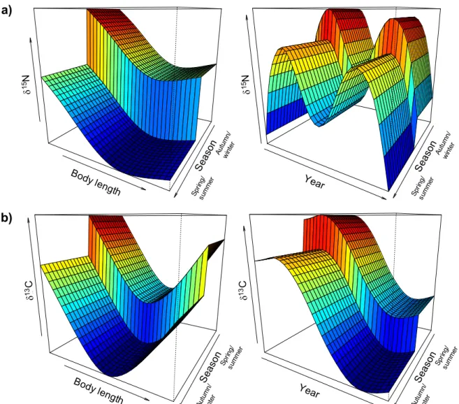
Figure S1 Visual representation of the categorical variable ‘season’ in GAMs, for a) nitrogen and b) carbon isotopic values. Graphs in b) have been rotated to show lower variable level in front. SeasonP ool Total.lengt h linear predict or SeasonP ool Total.lengt h linear predict or SeasonP ool Year linear predict or SeasonP ool Year linear predict or δ 15N 15Nδ δ 13C δ 13C Body length Body length Year Year Sea son a) b) Autu mn/ wint er Sprin g/ sum mer Sea son Autu mn/ wint er Sprin g/ sum mer Sea son Sprin g/ sum mer Autu mn/ wint er Sea son Sprin g/ sum mer Autu mn/ wint er
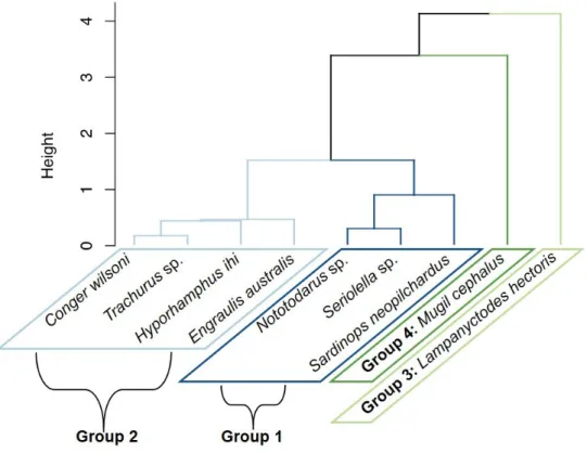
Figure S2 Dendrogram showingclustering of potential prey species. Ward’s correlation coefficient = 0.728, height indicates the cophenetic distance between members.
7
Figure S3 a) Isotopic values for weaned (≥170 cm body length) Delphinus delphis,
individuals represented as black dots) and their potential dietary source groups (displayed as mean ± 1 SD, with incorporated diet-to-tissue discrimination factors: 1.01 ± 0.37‰ (mean ± SD) for δ13C and 1.57 ± 0.52‰ for δ15N) including Epigonus crassicaudus (values obtained
from Sepúlveda et al. (2018)). Group 1: Sardinops neopilchardus, Seriolella sp.,
Nototodarus sp.; Group 2:Hyporhamphusihi, Trachurus sp., Congerwilsoni, Engraulis australis; Group 3:Lampanyctodes hectoris; Group 4:Mugil cephalus. b) Mixing polygon for data presented in a), showing individual dolphins (black dots) and potential dietary source groups (white dots). Black lines represent probability contours at 10% levels. By including E. crassicaudus, validation improves drastically with only 1 individual dolphin falling outside of the 95% mixing space.
REFERENCES
Jackson, A. L., Inger, R., Parnell, A. C. & Bearhop, S. 2011. Comparing isotopic niche widths among and within communities: SIBER – Stable Isotope Bayesian Ellipses in R. J. Anim. Ecol., 80, 595-602.
Layman, C. A., Arrington, D. A., Montaña, C. G. & Post, D. M. 2007. Can stable isotope ratios provide for community-wide measures of trophic structure? Ecology, 88, 42-48. Paul, D., Skrzypek, G. & Fórizs, I. 2007. Normalization of measured stable isotopic
compositions to isotope reference scales–a review. Rapid Commun. Mass Spectrom.,
21, 3006-3014.
Sepúlveda, F., Gálvez, P., Molina-Burgos, B. E. & Klarian, S. A. 2018. Hábitos alimentarios del besugo Epigonus crassicaudus combinando contenido estomacal e isótopos estables. Rev. Biol. Mar. Oceanogr., 53, 31-37.
12.5 15.0 17.5 20.0 -20 -18 -16 -14 a) δ 15N (‰) D. delphis Group 1 Group 2 Group 3 Group 4 E. crassicaudus 11 12 13 14 15 16 -20 -18 -16 -14 Species Group 1 Group 2 Group 3 Group 4 δ13C (‰) -22 -20 -18 -16 -14 -12 -10 10 12 14 16 18 20 22 δ13C (‰) δ 15N (‰) b) -22 -20 -18 -16 -14 -12 -10 0.0 0.2 0.4 0.6 0.8 1.0 1 0.8 0.6 0.4 0.2 0 22 20 18 16 14 12 10 -20 -18 -16 -14 20 17.5 15 12.5 Groups D. delphis 12.5 15.0 17.5 -20 -18 -16 -14 Species Group 1 Group 2 Group 3 Group 4 Group 5