Multiresolution Gray Scale and Rotation Invariant Texture Classification
with Local Binary Patterns
Timo Ojala, Matti Pietikäinen and Topi Mäenpää
Machine Vision and Media Processing Unit Infotech Oulu, University of Oulu
P.O.Box 4500, FIN - 90014 University of Oulu, Finland
{skidi, mkp, topiolli}@ee.oulu.fi http://www.ee.oulu.fi/research/imag/texture
Abstract. This paper presents a theoretically very simple yet efficient multiresolution approach to gray scale and rotation invariant texture classification based on local binary pat-terns and nonparametric discrimination of sample and prototype distributions. The method is based on recognizing that certain local binary patterns termed ‘uniform’ are fundamental prop-erties of local image texture, and their occurrence histogram proves to be a very powerful tex-ture featex-ture. We derive a generalized gray scale and rotation invariant operator presentation that allows for detecting the ‘uniform’ patterns for any quantization of the angular space and for any spatial resolution, and present a method for combining multiple operators for multires-olution analysis. The proposed approach is very robust in terms of gray scale variations, since the operator is by definition invariant against any monotonic transformation of the gray scale. Another advantage is computational simplicity, as the operator can be realized with a few oper-ations in a small neighborhood and a lookup table. Excellent experimental results obtained in true problems of rotation invariance, where the classifier is trained at one particular rotation angle and tested with samples from other rotation angles, demonstrate that good discrimination can be achieved with the occurrence statistics of simple rotation invariant local binary patterns. These operators characterize the spatial configuration of local image texture and the perfor-mance can be further improved by combining them with rotation invariant variance measures that characterize the contrast of local image texture. The joint distributions of these orthogonal measures are shown to be very powerful tools for rotation invariant texture analysis.
Keywords: nonparametric texture analysis Brodatz distribution histogram contrast Ref: TPAMI 112278
1 Introduction
Analysis of two-dimensional textures has many potential applications, for example in industrial surface inspection, remote sensing and biomedical image analysis, but only a limited number of examples of successful exploitation of texture exist. A major problem is that tex-tures in the real world are often not uniform, due to variations in orientation, scale, or other visual appearance. The gray scale invariance is often important due to uneven illumination or great within-class variability. In addition, the degree of computational complexity of most pro-posed texture measures is too high, as Randen and Husoy [33] concluded in in their recent extensive comparative study involving dozens of different spatial filtering methods: “A very useful direction for future research is therefore the development of powerful texture measures that can be extracted and classified with a low computational complexity”.
Most approaches to texture classification assume, either explicitly or implicitly, that the unknown samples to be classified are identical to the training samples with respect to spatial scale, orientation and gray scale properties. However, real world textures can occur at arbitrary spatial resolutions and rotations and they may be subjected to varying illumination conditions. This has inspired a collection of studies, which generally incorporate invariance with respect to one or at most two of the properties spatial scale, orientation and gray scale.
The first few approaches on rotation invariant texture description include generalized cooc-currence matrices [12], polarograms [11] and texture anisotropy [7]. Quite often an invariant approach has been developed by modifying a successful noninvariant approach such as MRF (Markov Random Field) model or Gabor filtering. Examples of MRF based rotation invariant techniques include the CSAR (circular simultaneous autoregressive) model by Kashyap and Khotanzad [17], the MRSAR (multiresolution simultaneous autoregressive) model by Mao and Jain [24], and the works of Chen and Kundu [6], Cohen et al. [9], and Wu and Wei [38]. In the case of feature based approaches such as filtering with Gabor wavelets or other basis func-tions, rotation invariance is realized by computing rotation invariant features from the filtered images or by converting rotation variant features to rotation invariant features [14][15][16][20][21][22][23][31][40]. Using a circular neighbor set, Porter and Canagarajah [32] presented rotation invariant generalizations for all three mainstream paradigms: wavelets,
GMRF and Gabor filtering. Utilizing similar circular neighborhoods Arof and Deravi obtained rotation invariant features with 1-D DFT transformation [2].
A number of techniques incorporating invariance with respect to both spatial scale and rotation have been presented [1][9][21][23][39][40]. The approach based on Zernike moments by Wang and Healey [37] is one of the first studies to include invariance with respect to all three properties, spatial scale, rotation, and gray scale. In his mid 90’s survey on scale and rota-tion invariant texture classificarota-tion Tan [36] called for more work on perspective projecrota-tion invariant texture classification, which has received a rather limited amount of attention [5][8][18].
This work focuses on gray scale and rotation invariant texture classification, which has been addressed by Chen and Kundu [6] and Wu and Wei [38]. Both studies approached gray scale invariance by assuming that the gray scale transformation is a linear function. This is a some-what strong simplification, which may limit the usefulness of the proposed methods. Chen and Kundu realized gray scale invariance by global normalization of the input image using histo-gram equalization. This is not a general solution, however, as global histohisto-gram equalization can not correct intraimage (local) gray scale variations.
In this paper, we propose a theoretically and computationally simple approach which is robust in terms of gray scale variations and which is shown to discriminate a large range of rotated textures efficiently. Extending our earlier work [28][29][30], we present a gray scale and rotation invariant texture operator based on local binary patterns. Starting from the joint distribution of gray values of a circularly symmetric neighbor set of pixels in a local neighbor-hood, we derive an operator that is by definition invariant against any monotonic transforma-tion of the gray scale. Rotatransforma-tion invariance is achieved by recognizing that this gray scale invariant operator incorporates a fixed set of rotation invariant patterns.
The main contribution of this work lies in recognizing that certain local binary texture pat-terns termed ‘uniform’ are fundamental properties of local image texture, and in developing a generalized gray scale and rotation invariant operator for detecting these ‘uniform’ patterns. The term ‘uniform’ refers to the uniform appearance of the local binary pattern, i.e. there is a limited number of transitions or discontinuities in the circular presentation of the pattern.
These ‘uniform’ patterns provide a vast majority, sometimes over 90%, of the 3x3 texture pat-terns in examined surface textures. The most frequent ‘uniform’ binary patpat-terns correspond to primitive microfeatures such as edges, corners and spots, hence they can be regarded as feature detectors that trigger for the best matching pattern.
The proposed texture operator allows for detecting ‘uniform’ local binary patterns at circu-lar neighborhoods of any quantization of the angucircu-lar space and at any spatial resolution. We derive the operator for a general case based on a circularly symmetric neighbor set of P mem-bers on a circle of radius R, denoting the operator as LBPP,Rriu2. Parameter P controls the quan-tization of the angular space, whereas R determines the spatial resolution of the operator. In addition to evaluating the performance of individual operators of a particular (P,R), we also propose a straightforward approach for multiresolution analysis, which combines the responses of multiple operators realized with different (P,R).
The discrete occurrence histogram of the ‘uniform’ patterns (i.e. the responses of the
LBPP,Rriu2 operator) computed over an image or a region of image is shown to be a very
pow-erful texture feature. By computing the occurrence histogram we effectively combine struc-tural and statistical approaches: the local binary pattern detects microstructures (e.g. edges, lines, spots, flat areas), whose underlying distribution is estimated by the histogram.
We regard image texture as a two-dimensional phenomenon characterized by two orthogo-nal properties, spatial structure (pattern) and contrast (the ‘amount’ of local image texture). In terms of gray scale and rotation invariant texture description, these two are an interesting pair: where spatial pattern is affected by rotation, contrast is not, and vice versa, where contrast is affected by the gray scale, spatial pattern is not. Consequently, as long as we want to restrict ourselves to pure gray scale invariant texture analysis, contrast is of no interest, as it depends on the gray scale.
The LBPP,Rriu2 operator is an excellent measure of the spatial structure of local image tex-ture, but it by definition discards the other important property of local image textex-ture, i.e. con-trast, since it depends on the gray scale. If only rotation invariant texture analysis is desired, i.e. gray scale invariance is not required, the performance of LBPP,Rriu2 can be further
enhanced by combining it with a rotation invariant variance measure VARP,R that characterizes the contrast of local image texture. We present the joint distribution of these two complemen-tary operators, LBPP,Rriu2/VARP,R, as a powerful tool for rotation invariant texture classifica-tion.
As the classification rule, we employ nonparametric discrimination of sample and prototype distributions based on a log-likelihood measure of the (dis)similarity of histograms, which frees us from making any, possibly erroneous, assumptions about the feature distributions.
The performance of the proposed approach is demonstrated with two experiments. Excel-lent results in both experiments demonstrate that the proposed texture operator is able to pro-duce from just one reference rotation angle a representation that allows for discriminating a large number of textures at other rotation angles. The operators are also computationally attrac-tive, as they can be realized with a few operations in a small neighborhood and a lookup table. The paper is organized as follows. The derivation of the operators and the classification principle are described in Section 2. Experimental results are presented in Section 3 and Sec-tion 4 concludes the paper.
2 Gray Scale and Rotation Invariant Local Binary Patterns
We start the derivation of our gray scale and rotation invariant texture operator by defining texture T in a local neighborhood of a monochrome texture image as the joint distribution of the gray levels of P (P>1) image pixels:
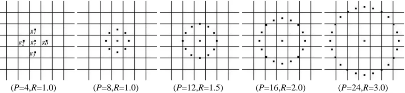
where gray value gc corresponds to the gray value of the center pixel of the local neighborhood and gp (p=0,...,P-1) correspond to the gray values of P equally spaced pixels on a circle of radius R (R>0) that form a circularly symmetric neighbor set. If the coordinates of gc are (0,0), then the coordinates of gp are given by (-Rsin(2πp/P), Rcos(2πp/P)). Fig. 1 illustrates
circu-larly symmetric neighbor sets for various (P,R). The gray values of neighbors which do not fall exactly in the center of pixels are estimated by interpolation.
2.1 Achieving Gray Scale Invariance
As the first step towards gray scale invariance we subtract, without losing information, the gray value of the center pixel (gc) from the gray values of the circularly symmetric neighbor-hood gp (p=0,...,P-1) giving:
Next, we assume that differences gp-gc are independent of gc, which allows us to factorize
Eq.(2):
In practice an exact independence is not warranted, hence the factorized distribution is only an approximation of the joint distribution. However, we are willing to accept the possible small loss in information, as it allows us to achieve invariance with respect to shifts in gray scale. Namely, the distribution t(gc) in Eq.(3) describes the overall luminance of the image, which is
unrelated to local image texture, and consequently does not provide useful information for tex-ture analysis. Hence, much of the information in the original joint gray level distribution (Eq.(1)) about the textural characteristics is conveyed by the joint difference distribution [29]:
This is a highly discriminative texture operator. It records the occurrences of various pat-terns in the neighborhood of each pixel in a P-dimensional histogram. For constant regions, the differences are zero in all directions. On a slowly sloped edge, the operator records the highest difference in the gradient direction and zero values along the edge, and for a spot the differ-ences are high in all directions.
Fig. 1. Circularly symmetric neighbor sets for different (P,R).
(P=8,R=1.0)
(P=4,R=1.0) (P=12,R=1.5) (P=16,R=2.0) (P=24,R=3.0)
gc g1 g2
g3 g0
T = t g( c,g0–gc,g1–gc, ,... gP–1–gc) (2)
T≈t g( )c t g( 0–gc,g1–gc, ,... gP–1–gc) (3)
Signed differences gp-gc are not affected by changes in mean luminance, hence the joint
dif-ference distribution is invariant against gray scale shifts. We achieve invariance with respect to the scaling of the gray scale by considering just the signs of the differences instead of their exact values:
where
By assigning a binomial factor 2p for each sign s(gp-g0), we transform Eq.(5) into a unique
LBPP,R number that characterizes the spatial structure of the local image texture:
The name ‘Local Binary Pattern’ reflects the functionality of the operator, i.e. a local neigh-borhood is thresholded at the gray value of the center pixel into a binary pattern. LBPP,R oper-ator is by definition invariant against any monotonic transformation of the gray scale, i.e. as long as the order of the gray values in the image stays the same, the output of the LBPP,R oper-ator remains constant.
If we set (P=8,R=1), we obtain LBP8,1 which is similar to the LBP operator we proposed in [28]. The two differences between LBP8,1 and LBP are: 1) the pixels in the neighbor set are indexed so that they form a circular chain, and 2) the gray values of the diagonal pixels are determined by interpolation. Both modifications are necessary to obtain the circularly symmet-ric neighbor set, which allows for deriving a rotation invariant version of LBPP,R.
2.2 Achieving Rotation Invariance
The LBPP,R operator produces 2P different output values, corresponding to the 2P different binary patterns that can be formed by the P pixels in the neighbor set. When the image is rotated, the gray values gp will correspondingly move along the perimeter of the circle around
g0. Since g0 is always assigned to be the gray value of element (0,R), to the right of gc, rotating
(5) T≈t s g( ( 0–gc),s g( 1–gc), ,... s g( P–1–gc))
s x( ) 1 x, ≥0
0 x, <0
= (6)
LBPP R, s g( p–g0)2p p=0
P–1
∑
a particular binary pattern naturally results in a different LBPP,R value. This does not apply to patterns comprising of only 0’s (or 1’s) which remain constant at all rotation angles. To remove the effect of rotation, i.e. to assign a unique identifier to each rotation invariant local binary pattern we define:
where ROR(x,i) performs a circular bit-wise right shift on the P-bit number x i times. In terms of image pixels Eq.(8) simply corresponds to rotating the neighbor set clockwise so many times that a maximal number of the most significant bits, starting from gP-1, are 0.
LBPP,Rri quantifies the occurrence statistics of individual rotation invariant patterns
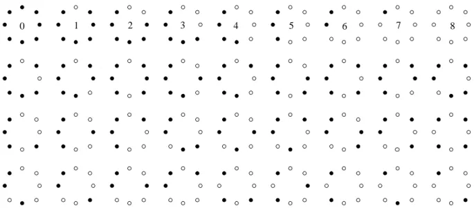
corre-sponding to certain microfeatures in the image, hence the patterns can be considered as feature detectors. Fig. 2 illustrates the 36 unique rotation invariant local binary patterns that can occur in the case of P=8, i.e. LBP8,Rri can have 36 different values. For example, pattern #0 detects bright spots, #8 dark spots and flat areas, and #4 edges. If we set R=1, LBP8,1ri corresponds to the gray scale and rotation invariant operator that we designated as LBPROT in [30].
LBPP Rri, = min ROR LBP{ ( P R, ,i) i= 0,1,...,P-1} (8)
0 1 2 3 4 5 6 7 8
Fig. 2. The 36 unique rotation invariant binary patterns that can occur in the circularly symmet-ric neighbor set of LBP8,Rri. Black and white circles correspond to bit values of 0 and 1 in the 8-bit output of the operator. The first row contains the nine ‘uniform’ patterns, and the numbers inside them correspond to their unique LBP8,Rriu2 codes.
2.3 Improved Rotation Invariance with ‘Uniform’ Patterns and Finer Quantization of the Angular Space
Our practical experience, however, has shown that LBPROT as such does not provide very good discrimination, as we also concluded in [30]. There are two reasons: the occurrence fre-quencies of the 36 individual patterns incorporated in LBPROT vary greatly, and the crude quantization of the angular space at 45o intervals.
We have observed that certain local binary patterns are fundamental properties of texture, providing vast majority, sometimes over 90%, of all 3x3 patterns present in the observed tex-tures. This is demonstrated in more detail in Section 3 with statistics of the image data used in the experiments. We call these fundamental patterns ‘uniform’ as they have one thing in com-mon, namely uniform circular structure that contains very few spatial transitions. ‘Uniform’ patterns are illustrated on the first row of Fig. 2. They function as templates for microstructures such as spot (0), flat area or dark spot (8) and edges of varying positive and negative curvature (1-7).
To formally define the ‘uniform’ patterns, we introduce a uniformity measure U(‘pattern’), which corresponds to the number of spatial transitions (bitwise 0/1 changes) in the ‘pattern’. For example, patterns 000000002 and 111111112 have U value of 0, while the other seven pat-terns in the first row of Fig. 2 have U value of 2, as there are exactly two 0/1 transitions in the pattern. Similarly, other 27 patterns have U value of at least 4. We designate patterns that have
U value of at most 2 as ‘uniform’ and propose the following operator for gray scale and
rota-tion invariant texture descriprota-tion instead of LBPP,Rri:
where
Superscript riu2 reflects the use of rotation invariant ‘uniform’ patterns that have U value of
LBPP Rriu2, s g( p–gc)
p=0 P–1
∑
if U LBP( P R, )≤2P+1 otherwise
= (9)
U LBP( P R, ) s g( P–1–gc)–s g( 0–gc) s g( p–gc)–s g( p–1–gc)
p=1 P–1
∑
+
at most 2. By definition exactly P+1 ‘uniform’ binary patterns can occur in a circularly sym-metric neighbor set of P pixels. Eq.(9) assigns a unique label to each of them, corresponding to the number of ‘1’ bits in the pattern (0->P), while the ‘nonuniform’ patterns are grouped under the ‘miscellaneous’ label (P+1). In Fig. 2 the labels of the ‘uniform’ patterns are denoted inside the patterns. In practice the mapping from LBPP,R to LBPP,Rriu2, which has P+2 distinct output values, is best implemented with a lookup table of 2P elements.
The final texture feature employed in texture analysis is the histogram of the operator out-puts (i.e. pattern labels) accumulated over a texture sample. The reason why the histogram of ‘uniform’ patterns provides better discrimination in comparison to the histogram of all individ-ual patterns comes down to differences in their statistical properties. The relative proportion of ‘nonuniform’ patterns of all patterns accumulated into a histogram is so small that their proba-bilities can not be estimated reliably. Inclusion of their noisy estimates in the (dis)similarity analysis of sample and model histograms would deteriorate performance.
We noted earlier that the rotation invariance of LBPROT (LBP8,1ri) is hampered by the crude 45o quantization of the angular space provided by the neighbor set of eight pixels. A straightforward fix is to use a larger P, since the quantization of the angular space is defined by (360o/P). However, certain considerations have to be taken into account in the selection of P. First, P and R are related in the sense that the circular neighborhood corresponding to a given R contains a limited number of pixels (e.g. 9 for R=1), which introduces an upper limit to the number of nonredundant sampling points in the neighborhood. Second, an efficient implemen-tation with a lookup of 2P elements sets a practical upper limit for P. In this study we explore P values up to 24, which requires a lookup table of 16 MB that can be easily managed by a mod-ern computer.
2.4 Rotation Invariant Variance Measures of the Contrast of Local Image Texture
The LBPP,Rriu2 operator is a gray scale invariant measure, i.e. its output is not affected by any monotonic transformation of the gray scale. It is an excellent measure of the spatial pat-tern, but it by definition discards contrast. If gray scale invariance is not required and we wanted to incorporate the contrast of local image texture as well, we can measure it with a
rota-tion invariant measure of local variance:
VARP,R is by definition invariant against shifts in gray scale. Since LBPP,Rriu2 and VARP,R
are complementary, their joint distribution LBPP,Rriu2/VARP,R is expected to be a very powerful
rotation invariant measure of local image texture. Note that even though we in this study restrict ourselves to using only joint distributions of LBPP,Rriu2 and VARP,R operators that have
the same (P,R) values, nothing would prevent us from using joint distributions of operators computed at different neighborhoods.
2.5 Nonparametric Classification Principle
In the classification phase, we evaluate the (dis)similarity of sample and model histograms as a test of goodness-of-fit, which is measured with a nonparametric statistical test. By using a nonparametric test we avoid making any, possibly erroneous, assumptions about the feature distributions. There are many well known goodness-of-fit statistics such as the chi-square sta-tistic and the G (log likelihood ratio) stasta-tistic [34]. In this study a test sample S was assigned to the class of the model M that maximized the log likelihood statistic:
where B is the number of bins, and Sb and Mb correspond to the sample and model probabilities at bin b, respectively. Eq.(12) is a straightforward simplification of the G (log likelihood ratio) statistic:
where the first term of the right hand expression can be ignored as a constant for a given S.
L is a nonparametric (pseudo-)metric that measures likelihoods that sample S is from
alter-native texture classes, based on exact probabilities of feature values of pre-classified texture
VARP R, 1 P
--- (gp–µ)2 p=0
P–1
∑
= , where µ 1
P
--- gp
p=0 P–1
∑
= (11)
L S M( , ) SblogMb
b=1 B
∑
= (12)
G S M( , ) 2 Sb Sb Mb
---log b=1
B
∑
2 [SblogSb–SblogMb]b=1 B
∑
models M. In the case of the joint distribution LBPP,Rriu2/VARP,R, Eq.(12) was extended in a
straightforward manner to scan through the two-dimensional histograms.
Sample and model distributions were obtained by scanning the texture samples and proto-types with the chosen operator, and dividing the distributions of operator outputs into histo-grams having a fixed number of B bins. Since LBPP,Rriu2 has a completely defined set of discrete output values (0 -> P+1), no additional binning procedure is required, but the operator outputs are directly accumulated into a histogram of P+2 bins. Each bin effectively provides an estimate of the probability of encountering the corresponding pattern in the texture sample or prototype. Spatial dependencies between adjacent neighborhoods are inherently incorporated in the histogram, because only a small subset of patterns can reside next to a given pattern.
Variance measure VARP,R has a continuous-valued output, hence quantization of its feature space is needed. This was done by adding together feature distributions for every single model image in a total distribution, which was divided into B bins having an equal number of entries. Hence, the cut values of the bins of the histograms corresponded to the (100/B) percentile of the combined data. Deriving the cut values from the total distribution and allocating every bin the same amount of the combined data guarantees that the highest resolution of quantization is used where the number of entries is largest and vice versa. The number of bins used in the quantization of the feature space is of some importance, as histograms with a too modest num-ber of bins fail to provide enough discriminative information about the distributions. On the other hand, since the distributions have a finite number of entries, a too large number of bins may lead to sparse and unstable histograms. As a rule of thumb, statistics literature often pro-poses that an average number of 10 entries per bin should be sufficient. In the experiments we set the value of B so that this condition is satisfied.
2.6 Multiresolution Analysis
We have presented general rotation-invariant operators for characterizing the spatial pattern and the contrast of local image texture using a circularly symmetric neighbor set of P pixels placed on a circle of radius R. By altering P and R we can realize operators for any quantiza-tion of the angular space and for any spatial resoluquantiza-tion. Multiresoluquantiza-tion analysis can be
accom-plished by combining the information provided by multiple operators of varying (P,R).
In this study we perform straightforward multiresolution analysis by defining the aggregate (dis)similarity as the sum of individual log-likelihoods computed from the responses of indi-vidual operators
where N is the number of operators, and Sn and Mn correspond to the sample and model histo-grams extracted with operator n (n=1,...,N), respectively. This expression is based on the addi-tivity property of the G statistic (Eq.(13)), i.e. the results of several G tests can be summed to yield a meaningful result. If X and Y are independent random events, and SX, SY, MX, and MY are the respective marginal distributions for S and M, then G(SXY,MXY) = G(SX,MX) +
G(SY,MY) [19].
Generally, the assumption of independence between different texture features does not hold. However, estimation of exact joint probabilities is not feasible due to statistical unreliability and computational complexity of large multidimensional histograms. For example, the joint histogram of LBP8,Rriu2, LBP16,Rriu2 and LBP24,Rriu2 would contain 4680 (10x18x26) cells. To satisfy the rule of thumb for statistical reliability, i.e. at least 10 entries per cell on average, the image should be of roughly (216+2R)(216+2R) pixels in size. Hence, high dimensional histo-grams would only be reliable with really large images, which renders them impractical. Large multidimensional histograms are also computationally expensive, both in terms of computing speed and memory consumption.
We have recently successfully employed this approach also in texture segmentation, where we quantitatively compared different alternatives for combining individual histograms for multiresolution analysis [26]. In this study we restrict ourselves to combinations of at most three operators.
3 Experiments
We demonstrate the performance of our approach with two different problems of rotation invariant texture analysis. Experiment #1 is replicated from a recent study on rotation invariant
LN L S( n,Mn)
n=1 N
∑
texture classification by Porter and Canagarajah [32], for the purpose of obtaining comparative results to other methods. Image data includes 16 source textures captured from the Brodatz album [4]. Considering this in conjunction with the fact that rotated textures are generated from the source textures digitally, this image data provides a slightly simplified but highly con-trolled problem for rotation invariant texture analysis. In addition to the original experimental setup, where training was based on multiple rotation angles, we also consider a more challeng-ing setup, where the texture classifier is trained at only one particular rotation angle and then tested with samples from other rotation angles.
Experiment #2 involves a new set of texture images [27], which have a natural tactile dimension and natural appearance of local intensity distortions caused by the tactile dimen-sion. Some source textures have large intra class variation in terms of color content, which results in highly different gray scale properties in the intensity images. Adding the fact that the textures were captured using three different illuminants of different color spectra, this image data presents a very realistic and challenging problem for illumination and rotation invariant texture analysis.
To incorporate three different spatial resolutions and three different angular resolutions, we realized LBPP,Rriu2 and VARP,R with (P,R) values of (8,1), (16,2), and (24,3) in the experiments. Corresponding circularly symmetric neighborhoods are illustrated in Fig. 1. In multiresolution analysis we use the three 2-resolution combinations and the one 3-resolution combination these three alternatives can form.
Before going into the experiments, we take a quick look at the statistical foundation of
LBPP,Rriu2. In the case of LBP8,Rriu2 we choose nine ‘uniform’ patterns out of the 36 possible
patterns, merging the remaining 27 under the ‘miscellaneous’ label. Similarly, in the case of
LBP16,Rriu2 we consider only 7% (17 out of 243) of the possible rotation invariant patterns.
Taking into account a minority of the possible patterns, and merging a majority of them, could imply that we are throwing away most of the pattern information. However, this is not the case, as the ‘uniform’ patterns appear to be fundamental properties of local image texture, as illus-trated by the numbers in Table 1.
In the case of the image data of Experiment #1, the nine ‘uniform’ patterns of LBP8,1riu2 contribute from 76.6% up to 91.8% of the total pattern data, averaging 87.2%. The most fre-quent individual pattern is symmetric edge detector 000011112 with 18.0% share, followed by 000111112 (12.8%) and 000001112 (11.8%), hence these three patterns contribute 42.6% of the textures. As expected, in the case of LBP16,1riu2 the 17 ‘uniform’ patterns contribute a smaller proportion of the image data, from 50.9% up to 76.4% of the total pattern data, averaging 66.9%. The most frequent pattern is the flat area/dark spot detector 11111111111111112 with 8.8% share.
The numbers for the image data of Experiment #2 are remarkably similar. The contribution of the nine ‘uniform’ patterns of LBP8,1riu2 totaled over the three illuminants (see Section 3.2.1) ranges from 82.4% to 93.3%, averaging 89.7%. The three most frequent patterns are again 000011112 (18.9%), 000001112 (15.2%) and 000111112 (14.5%), totalling 48.6% of the patterns. The contribution of the 17 ‘uniform’ patterns of LBP16,2riu2 ranges from 57.6% to Table 1: Proportions (%) of ‘uniform’ patterns of all patterns for each texture used in the experiments, and their average proportion over all textures.
Experiment #1 Experiment #2
P=8, R=1 P=16, R=2 P=24, R=3
Texture P=8R=1 P=16R=2 P=25R=3 Texture ‘inca’ ‘tl84’ ‘horizon’ total total total
canvas 84.8 58.5 41.2 canvas001 91.4 90.9 90.4 90.9 71.2 53.4
cloth 91.8 74.2 52.8 canvas002 92.6 91.7 91.1 91.8 73.2 54.2
cotton 88.9 67.0 46.3 canvas003 89.6 89.3 88.2 89.0 68.2 50.4
grass 85.5 63.3 45.6 canvas005 93.5 93.1 93.3 93.3 78.0 61.2
leather 87.7 66.6 49.1 canvas006 87.4 86.4 86.5 86.8 60.8 42.2
matting 89.5 72.0 55.8 canvas009 83.2 82.3 81.9 82.4 59.3 43.8
paper 89.2 70.9 52.9 canvas011 90.6 89.3 89.0 89.6 67.1 48.6
pigskin 87.6 67.9 50.9 canvas021 85.6 85.6 85.4 85.5 57.6 41.0
raffia 91.4 76.4 59.1 canvas022 92.3 91.1 91.0 91.4 78.1 65.0
rattan 86.1 68.5 52.4 canvas023 91.1 90.6 90.2 90.6 69.7 50.9
reptile 88.4 70.9 55.6 canvas025 93.2 92.8 92.7 92.9 76.1 55.0
sand 89.1 70.7 53.4 canvas026 92.2 91.8 91.5 91.8 68.0 47.8
straw 83.8 56.6 40.7 canvas031 93.0 92.5 92.4 92.6 74.3 55.8
weave 76.6 50.9 32.1 canvas032 89.8 88.8 89.4 89.3 66.4 49.0
wood 86.1 65.1 46.1 canvas033 92.8 92.1 91.8 92.2 75.0 56.2
wool 88.9 71.0 55.0 canvas035 90.4 90.1 89.4 90.0 68.4 50.4
AVERAGE 87.2 66.9 49.3 canvas038 91.0 89.7 89.8 90.1 71.4 54.6
canvas039 92.7 91.7 91.6 92.0 75.8 59.0
tile005 90.0 89.6 88.3 89.3 71.5 54.3
tile006 91.0 90.5 89.7 90.4 74.0 57.8
carpet002 82.8 83.6 81.1 82.5 65.5 55.6
carpet004 87.6 87.1 86.3 87.0 70.8 57.8
carpet005 92.2 91.6 91.0 91.6 79.6 67.9
carpet009 90.8 90.5 89.7 90.3 77.4 64.5
79.6%, averaging 70.7%. The most frequent patterns is again 11111111111111112 with 8.7% share. In the case of LBP24,3riu2 the 25 ‘uniform’ patterns contribute 54.0% of the local texture. The two most frequent patterns are the flat area/dark spot detector (all bits ‘1’) with 8.6% share and the bright spot detector (all bits ‘0’) with 8.2% share.
3.1 Experiment #1
In their comprehensive study, Porter and Canagarajah [32] presented three feature extrac-tion schemes for rotaextrac-tion invariant texture classificaextrac-tion, employing the wavelet transform, a circularly symmetric Gabor filter, and a Gaussian Markov Random Field with a circularly symmetric neighbor set. They concluded that the wavelet-based approach was the most accu-rate and exhibited the best noise performance, having also the lowest computational complex-ity.
3.1.1. Image Data and Experimental Setup
The image data included 16 texture classes from the Brodatz album [4] shown in Fig. 3. For each texture class there were eight 256x256 source images, of which the first was used for training the classifier, while the other seven images were used to test the classifier. Porter and Canagarajah created 180x180 images of rotated textures from these source images using bilin-ear interpolation. If the rotation angle was a multiple of 90 degrees (0o or 90o in the case of present ten rotation angles), a small amount of artificial blur was added to the images to simu-late the effect of blurring on rotation at other angles. It should be stressed that the source tex-tures were captured from sheets in the Brodatz album and that the rotated textex-tures were generated digitally from the source images. Consequently, the rotated textures do not have any local intensity distortions such as shadows, which could be caused when a real texture with a natural tactile dimension was rotated with respect to an illuminant and a camera. Thus, this image data provides a slightly simplified but highly controlled problem for rotation invariant texture analysis.
In the original experimental setup, the texture classifier was trained with several 16x16 sub-images extracted from the training image. This fairly small size of training samples increases the difficulty of the problem nicely. The training set comprised rotation angles 0o, 30o, 45o,
and 60o, while the textures for classification were presented at rotation angles 20o, 70o, 90o, 120o, 135o, and 150o. Consequently, the test data included 672 samples, 42 (6 angles x 7 images) for each of the 16 texture classes. Using a Mahalanobis distance classifier, Porter and Canagarajah reported 95.8% classification accuracy for the rotation invariant wavelet-based features as the best result.
3.1.2. Experimental Results
We started replicating the original experimental setup by dividing the 180x180 images of the four training angles (0o, 30o, 45o, and 60o) into 121 disjoint 16x16 subimages. In other Fig. 3. 180x180 samples of the 16 textures used in Experiment #1 at particular angles.
WOOL 0o
canvas 0o cloth 20o
matting 70o leather 60o
raffia 135o rattan 150o reptile 0o
pigskin 120o
sand 20o cotton 30o
paper 90o
grass 45o
wool 70o wood 60o
words we had 7744 training samples, 484 (4 angles x 121 samples) in each of the 16 texture classes. We first computed the histogram of the chosen operator for each of the 16x16 samples. Then we added the histograms of all samples belonging to a particular class into one big model histogram for this class, since the histograms of single 16x16 samples would have been too sparse to be reliable models. Also, using 7744 different models would have resulted in compu-tational overhead, for in the classification phase the sample histograms were compared to every model histogram. Consequently, we obtained 16 reliable model histograms containing 484(16-2R)2 entries (the operators have a R pixel border). The performance of the operators was evaluated with the 672 testing images. Their sample histograms contained (180-2R)2 entries, hence we did not have to worry about their stability.
Results in Table 2 correspond to the percentage of correctly classified samples of all testing samples. As expected, LBP16,2riu2 and LBP24,3riu2 clearly outperformed their simpler counter-part LBP8,1riu2, which had difficulties in discriminating strongly oriented textures, as misclas-sifications of rattan, straw and wood contributed 70 of the 79 misclassified samples. Interestingly, in all 79 cases the model of the true class ranked second right after the most sim-ilar model of a false class that led to misclassification. LBP16,2riu2 did much better, classifying all samples correctly except ten grass samples that were assigned to leather. Again, in all ten cases the model of the true class ranked second. LBP24,3riu2 provided further improvement by missing just five grass samples and a matting sample. In all six cases the model of the true class again ranked second.
Combining the LBPP,Rriu2 operator with the VARP,R operator, which did not too badly by itself, generally improved the performance. The lone exception was (24,3) where the addition of the poorly performing VAR24,3 only hampered the excellent discrimination by LBP24,3riu2. We see that LBP16,2riu2/VAR16,2 fell one sample short of a faultless result, as a straw sample at
90o angle was labeled as grass.
The results for single resolutions are so good that there is not much room for improvement by the multiresolution analysis, though two joint distributions provided a perfect classification.
The largest gain was achieved for the VARP,R operator, especially when VAR24,3 was excluded.
Note that we voluntarily discarded the knowledge that training samples come from four dif-ferent rotation angles, merging all sample histograms into a single model for each texture class. Hence the final texture model was an ‘average’ of the models of the four training angles, which actually decreased the performance to a certain extent. If we had used four separate models, one for each training angle, for example LBP16,2riu2/VAR16,2 would have provided a perfect
classification, and the classification error of LBP16,2riu2 would have been halved.
Even though a direct comparison to the results of Porter and Canagarajah may not be mean-ingful due to the different classification principle, the excellent results for our operators dem-onstrate their suitability for rotation invariant texture classification.
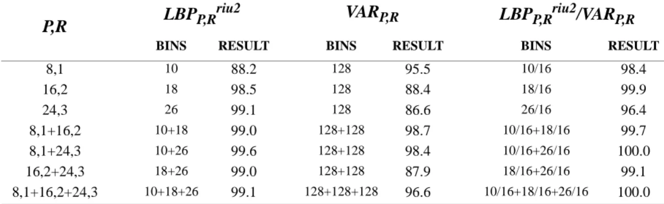
Table 3 presents results for a more challenging experimental setup, where the classifier was trained with samples of just one rotation angle and tested with samples of other nine rotation angles. We trained the classifier with the 121 16x16 samples extracted from the designated training image, again merging the histograms of the 16x16 samples of a particular texture class into one model histogram. The classifier was tested with the samples obtained from the other nine rotation angles of the seven source images reserved for testing purposes, totaling 1008 samples, 63 in each of the 16 texture classes. Note that the seven testing images in each texture class are physically different from the one designated training image, hence this setup is a true test for the texture operators’ ability to produce a rotation invariant representation of local Table 2: Classification accuracies (%) for the original experimental setup, where training is done with rotations 0o, 30o, 45o, and 60o.
P,R LBPP,R
riu2 VAR
P,R LBPP,Rriu2/VARP,R
BINS RESULT BINS RESULT BINS RESULT
8,1 10 88.2 128 95.5 10/16 98.4
16,2 18 98.5 128 88.4 18/16 99.9
24,3 26 99.1 128 86.6 26/16 96.4
8,1+16,2 10+18 99.0 128+128 98.7 10/16+18/16 99.7
8,1+24,3 10+26 99.6 128+128 98.4 10/16+26/16 100.0
16,2+24,3 18+26 99.0 128+128 87.9 18/16+26/16 99.1
image texture that also generalizes to physically different samples.
Training with just one rotation angle allows a more conclusive analysis of the rotation invariance of our operators. For example, it is hardly surprising that LBP8,1riu2 provides worst performace when the training angle is a multiple of 45o. Due to the crude quantization of the angular space the presentations learned at 0o, 45o, 90o, or 135o do not generalize that well to other angles.
Again, the importance of the finer quantization of the angular space shows, as LBP16,2riu2 and LBP24,3riu2 provide a solid performance with average classification accuracy of 98.3% and 98.5%, respectively. In the case of the 173 misclassifications by LBP16,2riu2 the model of the true class ranked always second. In the case of the 149 misclassifications by LBP24,3riu2 the Table 3: Classification accuracies (%) when training is done at just one rotation angle, and the average accuracy over the ten angles.
OPERATOR P,R BINS TRAINING ANGLE AVERAGE
0o 20o 30o 45o 60o 70o 90o 120o 135o 150o
LBPP,Rriu2
8,1 10 68.7 86.4 84.7 76.4 85.0 84.3 69.4 84.4 76.3 84.8 80.1
16,2 18 96.2 99.0 98.6 98.9 98.5 99.1 97.6 98.6 98.7 97.5 98.3
24,3 26 98.7 98.9 0.9 97.6 99.2 98.2 100 98.7 96.7 98.0 98.5
8,1+16,2 10+18 94.3 99.5 99.8 99.8 98.5 97.2 92.9 99.6 99.2 99.2 98.0
8,1+24,3 10+26 96.2 99.6 99.4 98.6 99.4 98.9 97.2 99.5 98.3 99.4 98.7
16,2+24,3 18+26 97.7 100 99.8 99.2 99.3 100 99.6 99.4 98.5 98.4 99.2
8,1+16,2+24,3 10+18+26 97.6 100 100 100 100 100 98.5 100 98.6 99.8 99.4
VARP,R
8,1 128 92.7 96.6 94.6 94.0 95.6 96.9 93.9 94.2 94.6 95.6 94.9
16,2 128 89.9 84.5 86.2 90.5 87.3 85.6 91.0 89.8 90.8 88.5 88.4
24,3 128 85.4 86.4 85.7 84.4 85.4 85.6 86.0 86.7 86.3 85.9 85.8
8,1+16,2 128+128 97.5 96.9 98.8 99.0 97.9 97.7 97.5 99.1 98.8 97.9 98.1
8,1+24,3 128+128 95.2 97.0 98.7 98.9 97.5 98.5 96.1 99.5 99.0 97.9 97.8
16,2+24,3 128+128 88.3 86.5 86.8 86.9 85.5 86.5 89.3 86.9 87.5 87.1 87.1
8,1+16,2+24,3 128+128+128 94.9 94.6 97.0 98.3 96.2 96.2 95.0 98.2 98.1 97.3 96.6
LBPriu2P,R/VARP,R
8,1 10/16 99.1 94.2 95.7 97.3 95.2 94.4 99.3 96.0 97.3 95.6 96.4
16,2 18/16 100 99.5 99.4 99.4 99.4 99.6 100 99.5 99.5 99.7 99.6
24,3 26/16 95.8 95.0 96.2 97.4 96.0 95.5 95.6 97.2 97.9 97.9 96.5
8,1+16,2 10/16+18/16 100 99.3 99.1 99.2 99.3 99.2 100 99.3 99.3 99.4 99.4
8,1+24,3 10/16+26/16 99.8 99.8 99.6 99.8 99.6 99.8 99.6 99.7 99.8 99.9 99.7
16,2+24,3 18/16+26/16 97.2 98.9 98.9 99.8 99.6 99.9 97.3 99.6 99.8 99.9 99.1
model of the true class ranked second 117 times and third 32 times.
There is a strong suspicion that the weaker results for LBP16,2riu2 at training angles 0o and 90o were due to the artificial blur added to the original images at angles 0o and 90o. The effect of the blur can also be seen in the results of the joint distributions LBP8,1riu2/VAR8,1 and
LBP16,2riu2/VAR16,2, which achieved best performance when the training angle is either 0o or 90o, the (16,2) joint operator providing in fact a perfect classification in these cases. Namely, when training was done at some other rotation angle, test angles 0o and 90o contributed most of the misclassified samples, actually all of them in the case of LBP16,2riu2/VAR16,2. Nevertheless,
the result for LBP16,2riu2/VAR16,2 is quite excellent, whereas LBP24,3riu2/VAR24,3 seems to
suf-fer from the poor discrimination of the variance measure.
Even though the results for multiresolution analysis generally exhibit improved discrimina-tion over single resoludiscrimina-tions, they also serve as a welcome reminder that the addidiscrimina-tion of inferior operator does not necessarily enhance the performance.
3.2 Experiment #2
3.2.1. Image Data and Experimental Setup
In this experiment we used textures from Outex, which is a publicly available (http://
www.outex.oulu.fi) framework for experimental evaluation of texture analysis algorithms [27].
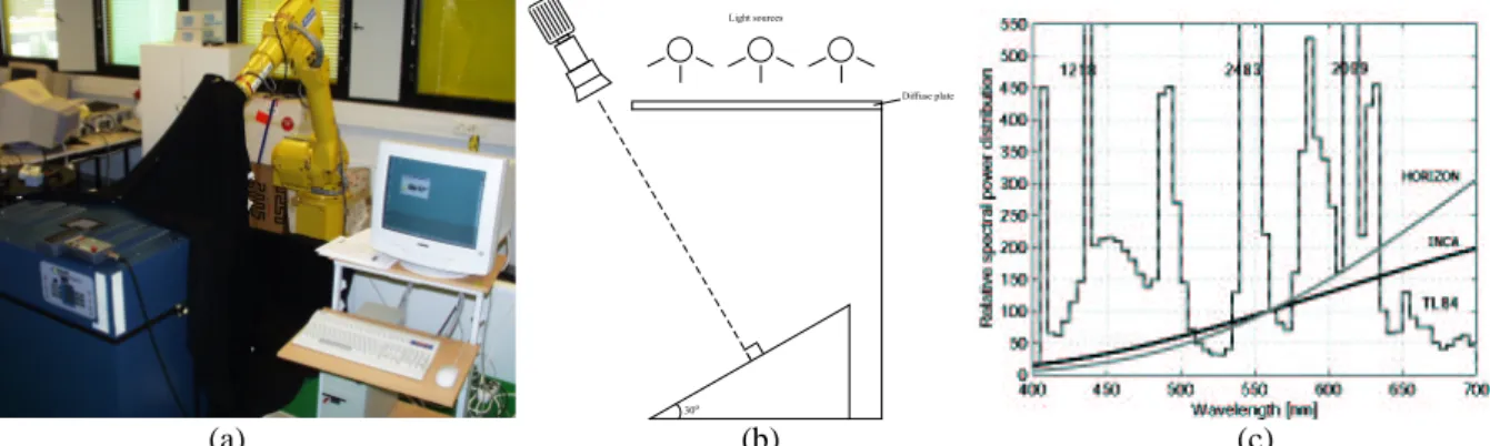
Outex provides a large collection of textures and ready-made test suites for different types of texture analysis problems, together with baseline results for well known published algorithms. The surface textures available in the Outex image database are captured using the setup shown in Fig. 4a. It includes a Macbeth SpectraLight II Luminare light source and a Sony DXC-755P three chip CCD camera attached to a robot arm. A workstation controls the light source for the purpose of switching on the desired illuminant, the camera for the purpose of selecting desired zoom dictating the spatial resolution, the robot arm for the purpose of rotating the camera into the desired rotation angle and the frame grabber for capturing 24-bit RGB images of size 538 (height) x 716 (width) pixels. The relative positions of a texture sample, illuminant and camera are illustrated in Fig 4b.
Each texture available at the site is captured using three different simulated illuminants pro-vided in the light source: 2300K horizon sunlight denoted as ‘horizon’, 2856K incandescent CIE A denoted as ‘inca’, and 4000K fluorescent tl84 denoted as ‘tl84’. The spectra of the illu-minants are shown in Fig. 4c. The camera is calibrated using the ‘inca’ illuminant. It should be noted that despite of the diffuse plate the imaging geometry is different for each illuminant, due to their different physical location in the light source. Each texture is captured using six spatial resolutions (100, 120, 300, 360, 500 and 600 dpi) and nine rotation angles (0o, 5o, 10o, 15o, 30o, 45o, 60o, 75o and 90o), hence 162 images are captured from each texture.
The frame grabber produces rectangular pixels, whose aspect ratio (height/width) is roughly 1.04. The aspect ratio is corrected by stretching the images in horizontal direction to size 538x746 using Matlab’s imresize command with bilinear interpolation. Bilinear interpolation is employed instead of bicubic, because the latter may introduce halos or extra noise around edges or in areas of high contrast, which would be harmful to texture analysis. Horizontal stretching is used instead of vertical size reduction, because sampling images captured by an interline transfer camera along scan lines produces less noise and digital artifacts than sam-pling across the scan lines.
In this study we used images captured at the 100 dpi spatial resolution. 24-bit RGB images were transformed into eight bit intensity images using the standard formula:
20 nonoverlapping 128x128 texture samples were extracted from each intensity image by
30o
Diffuse plate Light sources
Fig. 4. a) Imaging setup. b) Relative positions of texture sample, illuminant and camera. (c) Spectra of the illuminants.
(b)
(a) (c)
centering the 5x4 sampling grid so that equally many pixels were left over on each side of the sampling grid (13 pixels above and below, 53 pixels left and right).
To remove the effect of global first and second order gray scale properties, which are unrelated to local image texture, each 128x128 texture sample was individually normalized to have an average intensity of 128 and a standard deviation of 20. In every forthcoming experiment the
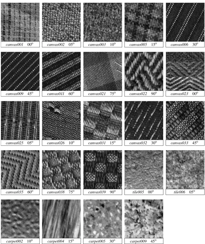
canvas006 30o canvas001 00o canvas002 05o canvas003 10o canvas005 15o
Fig. 5. 128x128 samples of the 24 textures used in Experiment #2 at particular angles. canvas009 45o canvas011 60o canvas021 75o canvas022 90o canvas023 00o
canvas025 05o canvas026 10o canvas031 15o canvas032 30o canvas033 45o
canvas035 60o canvas038 75o canvas039 90o tile005 00o tile006 05o
classifier was trained with the samples extracted from images captured using illuminant ‘inca’ and angle 0o (henceforth termed the reference textures).
We selected the 24 textures shown in Fig. 5. While selecting the textures, the underlying texture pattern was required to be roughly uniform over the whole source image, while local gray scale variations due to varying color properties of the source texture were allowed (e.g.
canvas023 and canvas033 shown in Fig. 6). Most of the texture samples are canvases with
strong directional structure. Some of them have a large tactile dimension (e.g. canvas025,
canvas033 and canvas038), which can induce considerable local gray scale distortions. Taking
variations caused by different spectra of the illuminants into account, we can conclude that this collection of textures presents a realistic and challenging problem for illumination and rotation invariant texture analysis.
The selection of textures was partly guided by the requirement that the reference textures could be separated from each other. This allowed quantifying our texture operators’ ability to discriminate rotated textures without any bias introduced by the inherent difficulty of the prob-lem. When the 480 samples (24 classes a’ 20) were randomly halved 100 times so that half of the 20 samples in each texture class served as models for training the classifier, and the other 10 samples were used for testing the classifier with the 3-NN method (sample was assigned to the class of the majority of the three most similar models), 99.4% average classification accu-racy was achieved with the simple rotation variant LBP8,1 operator (Eq.(7)). The performance loss incurred by considering just rotation invariant ‘uniform’ patterns is demonstrated by the Fig. 6. Intra class gray scale variations caused by varying color content of source textures.
93.2% average accuracy obtained with the corresponding rotation invariant operator LBP8,1riu2. LBP16,2riu2 and LBP24,3riu2 achieved average classification accuracies of 94.6% and 96.3%, respec-tively, in classifying the reference textures.
3.2.2. Experimental Results We considered two different setups:
Rotation invariant texture classification (test suite Outex_TC_00010): the classifier is trained with the reference textures (20 samples of illuminant ‘inca’ and angle 0o in each texture class), while the 160 samples of the the same illuminant ‘inca’ but the other eight other rotation angles in each texture class are used for testing the classifier. Hence, in this suite there are 480 (24x20) models and 3840 (24x20x8) validation samples in total.
Rotation and illuminant invariant texture classification (test suite Outex_TC_00012): the classifier is trained with the reference textures (20 samples of illuminant ‘inca’ and angle 0o in each texture class) and tested with all samples captured using illuminant ‘tl84’ (problem 000) and ‘horizon’ (problem 001). Hence, in both problems there are 480 (24x20) models and 4320 (24x20x9) validation samples in total.
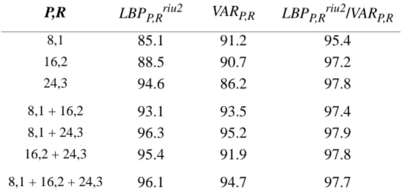
In Outex the performance of a texture classification algorithm is characterized with score (S), which corresponds to the percentage of correctly classified samples. Scores for the pro-posed operators, obtained using the 3-NN method, in rotation invariant texture classification (test suite Outex_TC_00010) are shown in Table 4. Of individual operators LBP24,3riu2 pro-duced the best score of 94.6%, which recalling the 96.3% score in the classification of refer-ence textures demonstrates the robustness of the operator with respect to rotation. LBP24,3riu2/
VAR24,3 achieved the best result of joint operators (97.8%), which is a considerable
improve-ment over either of the individual operators, underlining their compleimprove-mentary nature. Multires-olution analysis generally improved the performance, and the highest score (97.9%) was obtained with the combination of LBP8,1riu2/VAR8,1 and LBP24,3riu2/VAR24,3.
We offer the three employed combinations of (P,R) ((8,1), (16,2), and (24,3)) as a reason-able starting point for realizing the operators, but there is no guarantee that they produce the optimal operator for a given task. For example, when test suite Outex_TC_00010 was tackled with 189 LBPP,Rriu2 operators realized using (P=4, 5, ..., 24 ; R=1.0, 1.5, ..., 5.0), the best score of 97.2% was obtained with LBP22,4riu2. 32 of the 189 operators beat the 94.6% score obtained with LBP24,3riu2. 14 of those 32 operators were realized with (P=11...24 ; R=4.0) and they pro-duced eight highest scores (97.2 - 97.0%). Task or even texture class driven selection of texture operators could be conducted by optimizing cross validation classification of the training data, for example.
Table 5 shows the numbers of misclassified samples for each texture and rotation angle for LBP24,3riu2, VAR24,3 and LBP24,3riu2/VAR24,3, allowing detailed analysis of the discrimination of individual textures and the effect of rotation. LBP24,3riu2 classified seven out of the 24 classes completely correct, having most difficulties with canvas033 (48/160 misclassified, 19 assigned to canvas038, 16 to canvas031). LBP24,3riu2/VAR24,3 got 16 of the 24 classes correct, and well over half of the 2.2% error was contributed by 50 misclassified canvas038 samples. In 20 of the 24 classes, the joint operator did at least as well as either of the individual operators, dem-onstrating the usefulness of complementary analysis. However, the four exceptions (canvas005, canvas023, canvas033, tile005) remind that joint analysis is not guaranteed to provide the optimal performance. By studying the column totals and the contributions of indi-vidual rotation angles to misclassifications, we see that each operator had most misclassifica-Table 4: Scores (%) for the proposed texture operators in rotation invariant texture classification (test suite Outex_TC_00010).
P,R LBPP,Rriu2 VARP,R LBPP,Rriu2/VARP,R
8,1 85.1 91.2 95.4
16,2 88.5 90.7 97.2
24,3 94.6 86.2 97.8
8,1 + 16,2 93.1 93.5 97.4
8,1 + 24,3 96.3 95.2 97.9
16,2 + 24,3 95.4 91.9 97.8
tions at high rotation angles. For example, angle 90o contributed almost 30% of the misclassified samples in the case of LBP24,3riu2. This attributes to the different image acquisition properties of the interline transfer camera in horizontal and vertical directions.
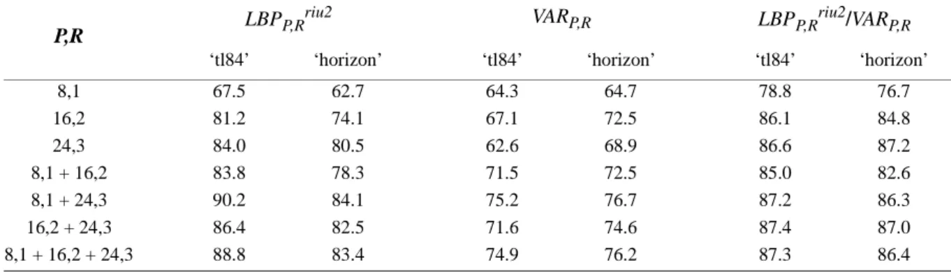
Scores in Table 6 illustrate the performance in rotation and illumination invariant texture classification (test suite Outex_TC_00012). The classifier was trained with the reference tex-tures (‘inca’, 0o) and tested with samples captured using a different illuminant. The scores for ‘horizon’ and ‘tl84’ include samples from all nine rotation angles, i.e. 180 samples of each tex-ture were used for testing the classifier.
We see that classification performance deteriorated clearly, when the classifier was evalu-ated with samples captured under different illumination than the reference textures used in training. It is difficult to quantify to which extent this is due to the differences in the spectral Table 5: The numbers of misclassified samples for each texture and rotation angle for LBP24,3riu2 (plain), VAR24,3 (italic) and LBP24,3riu2/VAR24,3 (bold) in the base problem. Column total % corresponds to the percentage of the column total of all misclassified samples. Only textures with misclassified samples are included.
Texture
Rotation angle
Total
5o 10o 15o 30 45o 60o 75o 90o
canvas001 . 3 . . 4 . . 5 . . 5 . . 2 . . 2 . . 6 . . 10 . . 37 .
canvas002 . . . . . . . . . . . . . . . 1 . . . . . . 1 . 1 1 .
canvas003 . 1 . . 1 . . . . . 2 . . 2 . . 1 . . 3 . . 4 . . 14 .
canvas005 . . . . . . . . . . . . . . . 1 . . 6 1 . 8 . 2 15 1 2
canvas011 . . . . . . . . . . . . 4 . . . . . 2 . . . . . 6 . .
canvas021 . 4 . . 3 . . 2 . . 3 . . 4 . . 1 . . 1 . . 2 . . 20 .
canvas023 . 11 . . 18 . . 16 . 2 18 2 . 18 1 . 17 1 . 14 . . 17 . 2 129 4
canvas025 . 1 . . 1 . . 2 . . 2 . . . . . . . . 1 . 3 . . 3 7 .
canvas031 . 1 . . 2 . . 1 . . 6 . 1 1 . 3 1 . 6 2 . 11 6 . 21 20 .
canvas032 . . . . . . . . . . 1 . 1 1 . 6 5 1 8 5 1 6 5 2 21 17 4
canvas033 3 6 2 3 8 5 2 10 6 2 12 6 9 13 7 9 8 5 10 10 10 10 11 9 48 78 50
canvas035 . . . 3 . . 3 1 . 2 1 . 2 1 1 2 . . 2 1 . 1 1 . 15 5 1
canvas038 . 2 . . 1 . . 3 . 2 3 . 4 2 . 6 5 . 9 5 . 9 3 . 30 24 .
canvas039 1 3 . 1 2 1 5 . 2 3 . 2 4 . 2 5 . 5 7 . 6 7 . 20 36 .
tile005 . 5 . . 3 1 1 2 2 . 6 1 1 6 2 1 5 1 . 1 1 . 9 3 3 37 11
tile006 . 6 1 . 5 . 1 5 1 1 7 1 2 5 1 2 8 . 3 5 3 5 6 4 14 47 11
carpet002 . . . . . . . . . . 1 . 1 2 . . 1 . . 3 . . 2 . 1 9 .
carpet004 . 3 . . 3 . . . . . 2 . 1 . . . . . 1 2 . . 1 . 2 11 .
carpet005 . . . . . . . . . . . . . . . . 1 . 2 . . 2 . . 4 1 .
carpet009 . 4 . . 5 1 . 2 1 1 8 . . 2 . . 3 . 1 5 . 1 7 . 3 36 2 LBP24,3riu2 4 1.9% 7 3.3% 9 4.3% 12 5.7% 28 13.3% 33 15.7% 55 26.2% 62 29.5% 209 94.6%
VAR24,3 50 9.4% 56 10.6% 54 10.2% 80 15.1% 63 11.9% 63 11.9% 72 13.6% 92 17.4% 530 86.2% LBP24,3riu2/VAR24,3 3 3.5% 7 8.2% 10 11.8% 10 11.8% 12 14.1% 8 9.4% 15 17.7% 20 23.5% 85 97.8%
properties of the illuminants affecting the colors of textures, and to which extent due to the dif-ferent imaging geometries of the illuminants affecting the appearance of local distortions caused by the tactile dimension of textures.
In terms of rotation and illumination invariant classification canvas038 was the most diffi-cult texture for LBP24,3riu2 (143/180 ‘tl84’ and 178/180 ‘horizon’ samples misclassified) and LBP24,3riu2/VAR24,3 (140/180 ‘tl84’ and 102/180 ‘horizon’ samples misclassified). This is easy to understand when looking at three different samples of canvas038 in Fig. 6, which illustrate the prominent tactile dimension of canvas038 and the effect it has on local texture structure under different illumination conditions.
For comparison purposes we implemented the wavelet-based rotation invariant features proposed by Porter and Canagarajah, which they concluded to be a favorable approach over Gabor-based and GMRF-based rotation invariant features [32]. We extracted the features using two different image areas, the 16x16 suggested by Porter and Canagarajah and 128x128. As classifier we used the Mahalanobis distance classifier, just like Porter and Canagarajah. Table 6: Scores (%) for the proposed operators in rotation and illumination invariant texture classification (test suite Outex_TC_00012). The classifier is trained with reference textures (illuminant ‘inca’) and tested with samples captured using illuminants ‘tl84’ (problem 000) and ‘horizon’ (problem 001).
P,R LBPP,R
riu2 VAR
P,R LBPP,Rriu2/VARP,R
‘tl84’ ‘horizon’ ‘tl84’ ‘horizon’ ‘tl84’ ‘horizon’
8,1 67.5 62.7 64.3 64.7 78.8 76.7
16,2 81.2 74.1 67.1 72.5 86.1 84.8
24,3 84.0 80.5 62.6 68.9 86.6 87.2
8,1 + 16,2 83.8 78.3 71.5 72.5 85.0 82.6
8,1 + 24,3 90.2 84.1 75.2 76.7 87.2 86.3
16,2 + 24,3 86.4 82.5 71.6 74.6 87.4 87.0
8,1 + 16,2 + 24,3 88.8 83.4 74.9 76.2 87.3 86.4
Fig. 7. Three samples of canvas038: a) ‘inca’, 0o; b) ‘horizon’, 45o; c) ‘tl84’, 90o.
(b)
Table 7 shows the scores for the wavelet-based features extracted with image area 128x128, since they provided slightly better performance than the features extracted with image area 16x16. When these features were employed in classifying the reference textures using 100 ran-dom halvings of the samples into training and testing sets, an average classification accuracy of 84.9% was obtained.
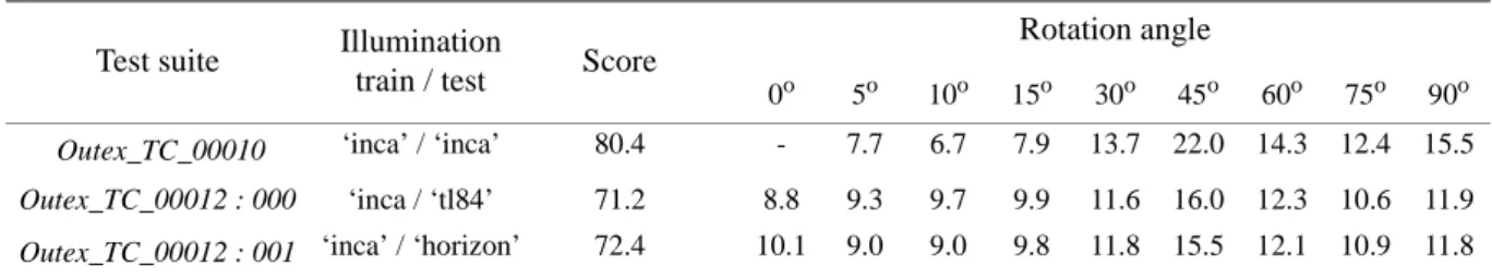
In the rotation invariant classification (test suite Outex_TC_00010) the wavelet-based based features achieved score of 80.4%, which is clearly lower than the scores obtained with the pro-posed operators. Wavelet-based features appeared to tolerate illumination changes moderately well, as demonstrated by the scores for the rotation and illumination invariant classification (test suite Outex_TC_00012, problems 000 and 001).
Table 7 also shows the percentages of misclassifications contributed by each rotation angle. We observe that 45o contributed the largest number of misclassified samples in all three cases. This is expected, for the rotation invariance of wavelet-based features is achieved by averaging horizontal and vertical information by grouping together LH and HL channels in each level of decomposition [32], which results in the weakest estimate in the 45o direction.
In rotation invariant classification (test suite Outex_TC_00010) wavelet-based features had most difficulties in discriminating textures canvas035 (86/160 samples misclassified),
canvas023 (78/160), canvas01 (76/160) and canvas033 (72/160). In rotation and illumination
invariant classification (test suite Outex_TC_00012) the highest classification errors were obtained for canvas11 (158/180 ‘tl84’ and 163/180 ‘horizon’ samples misclassified).
4 Discussion
We presented a theoretically and computationally simple yet efficient multiresolution Table 7: Scores (%) for the wavelet-based rotation invariant features proposed by Porter and Canagarajah and the percentages of misclassifications contributed by each rotation angle.
Test suite Illumination
train / test Score
Rotation angle
0o 5o 10o 15o 30o 45o 60o 75o 90o Outex_TC_00010 ‘inca’ / ‘inca’ 80.4 - 7.7 6.7 7.9 13.7 22.0 14.3 12.4 15.5 Outex_TC_00012 : 000 ‘inca / ‘tl84’ 71.2 8.8 9.3 9.7 9.9 11.6 16.0 12.3 10.6 11.9 Outex_TC_00012 : 001 ‘inca’ / ‘horizon’ 72.4 10.1 9.0 9.0 9.8 11.8 15.5 12.1 10.9 11.8