What Are Single-Year and Multiyear
Estimates?
Understanding Period Estimates
The ACS produces period estimates of socioeconomic and housing characteristics. It is designed to provide estimates that describe the average characteristics of an area over a specifi c time period. In the case of ACS single-year estimates, the period is the calendar year (e.g., the 2007 ACS covers January through December 2007). In the case of ACS multiyear estimates, the period is either 3 or 5 calendar years (e.g., the 2005– 2007 ACS estimates cover January 2005 through December 2007, and the 2006–2010 ACS estimates cover January 2006 through December 2010). The ACS multiyear estimates are similar in many ways to the ACS single-year estimates, however they encompass a longer time period. As discussed later in this appendix, the diff erences in time periods between single-year and multiyear ACS estimates aff ect decisions about which set of estimates should be used for a particular analysis.
While one may think of these estimates as representing average characteristics over a single calendar year or multiple calendar years, it must be remembered that the 1-year estimates are not calculated as an average of 12 monthly values and the multiyear estimates are not calculated as the average of either 36 or 60 monthly values. Nor are the multiyear estimates calculated as the average of 3 or 5 single-year estimates. Rather, the ACS collects survey information continuously nearly every day of the year and then aggregates the results over a specifi c time period—1 year, 3 years, or 5 years. The data collection is spread evenly across the entire period represented so as not to over-represent any particular month or year within the period.
Because ACS estimates provide information about the characteristics of the population and housing for areas over an entire time frame, ACS single-year and multiyear estimates contrast with “point-in-time” estimates, such as those from the decennial census long-form samples or monthly employment estimates
from the Current Population Survey (CPS), which are designed to measure characteristics as of a certain date or narrow time period. For example, Census 2000 was designed to measure the characteristics of the population and housing in the United States based upon data collected around April 1, 2000, and thus its data refl ect a narrower time frame than ACS data. The monthly CPS collects data for an even narrower time frame, the week containing the 12th of each month.
Implications of Period Estimates
Most areas have consistent population characteristics throughout the calendar year, and their period
estimates may not look much diff erent from estimates that would be obtained from a “point-in-time” survey design. However, some areas may experience changes in the estimated characteristics of the population, depending on when in the calendar year measurement occurred. For these areas, the ACS period estimates (even for a single-year) may noticeably diff er from “point-in-time” estimates. The impact will be more noticeable in smaller areas where changes such as a factory closing can have a large impact on population characteristics, and in areas with a large physical event such as Hurricane Katrina’s impact on the New Orleans area. This logic can be extended to better interpret 3-year and 5-3-year estimates where the periods involved are much longer. If, over the full period of time (for example, 36 months) there have been major or consistent changes in certain population or housing characteristics for an area, a period estimate for that area could diff er markedly from estimates based on a “point-in-time” survey.
An extreme illustration of how the single-year estimate could diff er from a “point-in-time” estimate within the year is provided in Table 1. Imagine a town on the Gulf of Mexico whose population is dominated by retirees in the winter months and by locals in the summer months. While the percentage of the population in the labor force across the entire year is about 45 percent (similar in concept to a period estimate), a “point-in-time” estimate for any particular month would yield estimates ranging from 20 percent to 60 percent.
Understanding and Using ACS Single-Year and Multiyear Estimates
Appendix 1.
Table 1. Percent in Labor Force—Winter Village
Source: U.S. Census Bureau, Artifi cial Data.
Month
Jan. Feb. Mar. Apr. May Jun. Jul. Aug. Sept. Oct. Nov. Dec.
The important thing to keep in mind is that ACS single-year estimates describe the population and characteristics of an area for the full year, not for any specifi c day or period within the year, while ACS multiyear estimates describe the population and characteristics of an area for the full 3- or 5-year period, not for any specifi c day, period, or year within the multiyear time period.
Release of Single-Year and Multiyear Estimates
The Census Bureau has released single-year estimates from the full ACS sample beginning with data from the 2005 ACS. ACS 1-year estimates are published annually for geographic areas with populations of 65,000 or more. Beginning in 2008 and encompassing 2005–2007, the Census Bureau will publish annual ACS 3-year estimates for geographic areas with populations of 20,000 or more. Beginning in 2010, the Census Bureau will release ACS 5-year estimates
(encompassing 2005–2009) for all geographic areas —down to the tract and block group levels. While eventually all three data series will be available each year, the ACS must collect 5 years of sample before that fi nal set of estimates can be released. This means that in 2008 only 1-year and 3-year estimates are available for use, which means that data are only available for areas with populations of 20,000 and greater.
New issues will arise when multiple sets of multiyear estimates are released. The multiyear estimates released in consecutive years consist mostly of overlapping years and shared data. As shown in Table 2, consecutive 3-year estimates contain 2 years of overlapping coverage (for example, the 2005–2007 ACS estimates share 2006 and 2007 sample data with the 2006–2008 ACS estimates) and consecutive 5-year estimates contain 4 years of overlapping coverage.
Table 2. Sets of Sample Cases Used in Producing ACS Multiyear Estimates
Type of estimate Year of Data Release
2008 2009 2010 2011 2012
Years of Data Collection 3-year
estimates 2005–2007 2006–2008 2007–2009 2008–2010 2009–2011 5-year
estimates Not Available Not Available 2005–2009 2006–2010 2007–2011
Diff erences Between Single-Year and
Multi-year ACS Estimates
Currency
Single-year estimates provide more current informa-tion about areas that have changing populainforma-tion and/or housing characteristics because they are based on the most current data—data from the past year. In contrast, multiyear estimates provide less current information because they are based on both data from the previous year and data that are 2 and 3 years old. As noted ear-lier, for many areas with minimal change taking place, using the “less current” sample used to produce the multiyear estimates may not have a substantial infl u-ence on the estimates. However, in areas experiencing major changes over a given time period, the multiyear estimates may be quite diff erent from the single-year estimates for any of the individual years. Single-year and multiyear estimates are not expected to be the same because they are based on data from two dif-ferent time periods. This will be true even if the ACS
single year is the midyear of the ACS multiyear period (e.g., 2007 single year, 2006–2008 multiyear).
For example, suppose an area has a growing Hispanic population and is interested in measuring the percent of the population who speak Spanish at home. Table 3 shows a hypothetical set of 1-year and 3-year esti-mates. Comparing data by release year shows that for an area such as this with steady growth, the 3-year estimates for a period are seen to lag behind the esti-mates for the individual years.
Reliability
Multiyear estimates are based on larger sample sizes and will therefore be more reliable. The 3-year esti-mates are based on three times as many sample cases as the 1-year estimates. For some characteristics this increased sample is needed for the estimates to be reliable enough for use in certain applications. For other characteristics the increased sample may not be necessary.
Table 3. Example of Diff erences in Single- and Multiyear Estimates—Percent of Population Who Speak Spanish at Home
Year of data
release 1-year estimates 3-year estimates
Time period Estimate Time period Estimate
2003 2002 13.7 2000–2002 13.4
2004 2003 15.1 2001–2003 14.4
2005 2004 15.9 2002–2004 14.9
2006 2005 16.8 2003–2005 15.9
the estimates. All of these factors, along with an understanding of the diff erences between single-year and multiyear ACS estimates, should be taken into con-sideration when deciding which set of estimates to use.
Understanding Characteristics
For users interested in obtaining estimates for small geographic areas, multiyear ACS estimates will be the only option. For the very smallest of these areas (less than 20,000 population), the only option will be to use the 5-year ACS estimates. Users have a choice of two sets of multiyear estimates when analyzing data for small geographic areas with populations of at least 20,000. Both 3-year and 5-year ACS estimates will be available. Only the largest areas with populations of 65,000 and more receive all three data series. The key trade-off to be made in deciding whether to use single-year or multiyear estimates is between currency and precision. In general, the single-year estimates are preferred, as they will be more relevant to the current conditions. However, the user must take into account the level of uncertainty present in the single-year estimates, which may be large for small subpopulation groups and rare characteristics. While single-year estimates off er more current estimates, they also have higher sampling variability. One mea-sure, the coeffi cient of variation (CV) can help you determine the fi tness for use of a single-year estimate in order to assess if you should opt instead to use the multiyear estimate (or if you should use a 5-year esti-mate rather than a 3-year estiesti-mate). The CV is calcu-lated as the ratio of the standard error of the estimate to the estimate, times 100. A single-year estimate with a small CV is usually preferable to a multiyear estimate as it is more up to date. However, multiyear estimates are an alternative option when a single-year estimate has an unacceptably high CV.
Multiyear estimates are the only type of estimates available for geographic areas with populations of less than 65,000. Users may think that they only need to use multiyear estimates when they are working with small areas, but this isn’t the case. Estimates for large geographic areas benefi t from the increased sample resulting in more precise estimates of population and housing characteristics, especially for subpopulations within those areas.
In addition, users may determine that they want to use single-year estimates, despite their reduced reliability, as building blocks to produce estimates for meaning-ful higher levels of geography. These aggregations will similarly benefi t from the increased sample sizes and gain reliability.
Deciding Which ACS Estimate to Use
Three primary uses of ACS estimates are to under-stand the characteristics of the population of an area for local planning needs, make comparisons across areas, and assess change over time in an area. Local planning could include making local decisions such as where to locate schools or hospitals, determining the need for services or new businesses, and carrying out transportation or other infrastructure analysis. In the past, decennial census sample data provided the most comprehensive information. However, the currency of those data suff ered through the intercensal period, and the ability to assess change over time was limited. ACS estimates greatly improve the currency of data for understanding the characteristics of housing and population and enhance the ability to assess change over time.
Several key factors can guide users trying to decide whether to use single-year or multiyear ACS estimates for areas where both are available: intended use of the estimates, precision of the estimates, and currency of
Table 4 illustrates how to assess the reliability of 1-year estimates in order to determine if they should be used. The table shows the percentage of households where Spanish is spoken at home for ACS test coun-ties Broward, Florida, and Lake, Illinois. The standard errors and CVs associated with those estimates are also shown.
In this illustration, the CV for the single-year estimate in Broward County is 1.0 percent (0.2/19.9) and in Lake County is 1.3 percent (0.2/15.9). Both are suf-fi ciently small to allow use of the more current single-year estimates.
Single-year estimates for small subpopulations (e.g., families with a female householder, no husband, and related children less than 18 years) will typically have larger CVs. In general, multiyear estimates are prefer-able to single-year estimates when looking at estimates for small subpopulations.
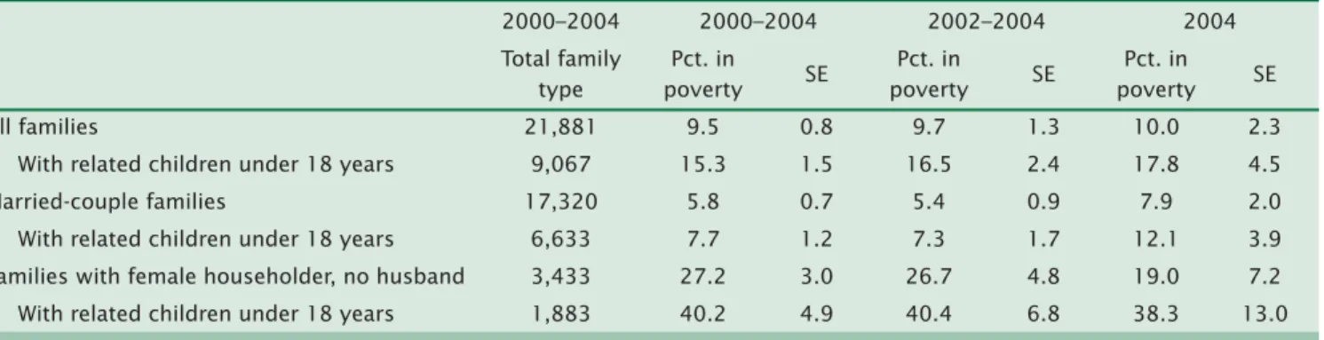
For example, consider Sevier County, Tennessee, which had an estimated population of 76,632 in 2004 accord-ing to the Population Estimates Program. This popula-tion is larger than the Census Bureau’s 65,000-population requirement for publishing 1-year esti-mates. However, many subpopulations within this geographic area will be much smaller than 65,000. Table 5 shows an estimated 21,881 families in Sevier County based on the 2000–2004 multiyear estimate; but only 1,883 families with a female householder, no
husband present, with related children under 18 years. Not surprisingly, the 2004 ACS estimate of the poverty rate (38.3 percent) for this subpopulation has a large standard error (SE) of 13.0 percentage points. Using this information we can determine that the CV is 33.9 percent (13.0/38.3).
For such small subpopulations, users obtain more precision using the 3-year or 5-year estimate. In this example, the 5-year estimate of 40.2 percent has an SE of 4.9 percentage points that yields a CV of 12.2 percent (4.9/40.2), and the 3-year estimate of 40.4 per-cent has an SE of 6.8 perper-centage points which yields a CV of 16.8 percent (6.8/40.4).
Users should think of the CV associated with an estimate as a way to assess “fi tness for use.” The CV threshold that an individual should use will vary based on the application. In practice there will be many estimates with CVs over desirable levels. A general guideline when working with ACS estimates is that, while data are available at low geographic levels, in situations where the CVs for these estimates are high, the reliability of the estimates will be improved by aggregating such estimates to a higher geographic level. Similarly, collapsing characteristic detail (for example, combining individual age categories into broader categories) can allow you to improve the reli-ability of the aggregate estimate, bringing the CVs to a more acceptable level.
Table 4. Example of How to Assess the Reliability of Estimates—Percent of Population Who Speak Spanish at Home
County Estimate Standard error Coeffi cient of
variation
Broward County, FL 19.9 0.2 1.0
Lake County, IL 15.9 0.2 1.3
Table 5. Percent in Poverty by Family Type for Sevier County, TN
2000–2004 2000–2004 2002–2004 2004 Total family
type
Pct. in
poverty SE
Pct. in
poverty SE
Pct. in poverty SE
All families 21,881 9.5 0.8 9.7 1.3 10.0 2.3
With related children under 18 years 9,067 15.3 1.5 16.5 2.4 17.8 4.5
Married-couple families 17,320 5.8 0.7 5.4 0.9 7.9 2.0
With related children under 18 years 6,633 7.7 1.2 7.3 1.7 12.1 3.9 Families with female householder, no husband 3,433 27.2 3.0 26.7 4.8 19.0 7.2 With related children under 18 years 1,883 40.2 4.9 40.4 6.8 38.3 13.0
Source: U.S. Census Bureau, Multiyear Estimates Study data. Source: U.S. Census Bureau, Multiyear Estimates Study data.
Assessing Change
Users are encouraged to make comparisons between sequential single-year estimates. Specifi c guidance on making these comparisons and interpreting the results are provided in Appendix 4. Starting with the 2007 ACS, a new data product called the comparison profi le will do much of the statistical work to identify statisti-cally signifi cant diff erences between the 2007 ACS and the 2006 ACS.
As noted earlier, caution is needed when using mul-tiyear estimates for estimating year-to-year change in a particular characteristic. This is because roughly two-thirds of the data in a 3-year estimate overlap with the data in the next year’s 3-year estimate (the over-lap is roughly four-fi fths for 5-year estimates). Thus, as shown in Figure 1, when comparing 2006–2008 3-year estimates with 2007–2009 3-year estimates, the diff erences in overlapping multiyear estimates are driven by diff erences in the nonoverlapping years. A data user interested in comparing 2009 with 2008 will not be able to isolate those diff erences using these two successive 3-year estimates. Figure 1 shows that the diff erence in these two estimates describes the diff er-ence between 2009 and 2006. While the interpretation of this diff erence is diffi cult, these comparisons can be made with caution. Users who are interested in com-paring overlapping multiyear period estimates should refer to Appendix 4 for more information.
Making Comparisons
Often users want to compare the characteristics of one area to those of another area. These comparisons can be in the form of rankings or of specifi c pairs of com-parisons. Whenever you want to make a comparison between two diff erent geographic areas you need to take the type of estimate into account. It is important that comparisons be made within the same estimate type. That is, 1-year estimates should only be com-pared with other 1-year estimates, 3-year estimates should only be compared with other 3-year estimates, and 5-year estimates should only be compared with other 5-year estimates.
You certainly can compare characteristics for areas with populations of 30,000 to areas with populations of 100,000 but you should use the data set that they have in common. In this example you could use the 3-year or the 5-year estimates because they are available for areas of 30,000 and areas of 100,000.
Figure 1. Data Collection Periods for 3–Year Estimates
Period
Jan. Dec. 2006
Jan. Dec. 2007
Jan. Dec. 2008
Jan. Dec. 2009 2007–2009
2006–2008
Figure 2. Civilian Veterans, County X Single-Year, Multiyear Estimates
15,000 15,500 16,000 16,500 17,000 17,500 18,000 18,500 19,000 19,500 20,000
2007 2006–2008
2008 2007–2009 2006–2010
2009 2008–2010 2007–2011
2010 2009–2011 2008–2012
2011 2010–2012
2012
Period
Estimated Civilian V
eterans
1-year estimate 3-year estimate 5-year estimate Variability in single-year estimates for smaller areas
(near the 65,000-publication threshold) and small sub-groups within even large areas may limit the ability to examine trends. For example, single-year estimates for a characteristic with a high CV vary from year to year because of sampling variation obscuring an underlying trend. In this case, multiyear estimates may be useful for assessing an underlying, long-term trend. Here again, however, it must be recognized that because the multiyear estimates have an inherent smoothing, they will tend to mask rapidly developing changes. Plotting the multiyear estimates as representing the middle year is a useful tool to illustrate the smoothing eff ect
of the multiyear weighting methodology. It also can be used to assess the “lagging eff ect” in the multiyear estimates. As a general rule, users should not consider a multiyear estimate as a proxy for the middle year of the period. However, this could be the case under some specifi c conditions, as is the case when an area is expe-riencing growth in a linear trend.
As Figure 2 shows, while the single-year estimates fl uctuate from year to year without showing a smooth trend, the multiyear estimates, which incorporate data from multiple years, evidence a much smoother trend across time.
Summary of Guidelines
Multiyear estimates should, in general, be used when single-year estimates have large CVs or when the preci-sion of the estimates is more important than the cur-rency of the data. Multiyear estimates should also be used when analyzing data for smaller geographies and smaller populations in larger geographies. Multiyear estimates are also of value when examining change over nonoverlapping time periods and for smoothing data trends over time.
Single-year estimates should, in general, be used for larger geographies and populations when currency is more important than the precision of the estimates. Single-year estimates should be used to examine year-to-year change for estimates with small CVs. Given the availability of a single-year estimate, calculating the CV provides useful information to determine if the single-year estimate should be used. For areas believed to be experiencing rapid changes in a characteristic, single-year estimates should generally be used rather than multiyear estimates as long as the CV for the single-year estimate is reasonable for the specifi c usage. Local area variations may occur due to rapidly
occurring changes. As discussed previously, multiyear estimates will tend to be insensitive to such changes when they fi rst occur. Single-year estimates, if
associ-ated with suffi ciently small CVs, can be very valuable in identifying and studying such phenomena. Graph-ing trends for such areas usGraph-ing sGraph-ingle-year, 3-year, and 5-year estimates can take advantage of the strengths of each set of estimates while using other estimates to compensate for the limitations of each set.
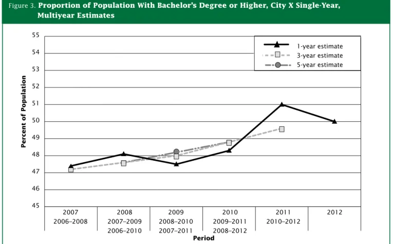
Figure 3 provides an illustration of how the various ACS estimates could be graphed together to better under-stand local area variations.
The multiyear estimates provide a smoothing of the upward trend and likely provide a better portrayal of the change in proportion over time. Correspondingly, as the data used for single-year estimates will be used in the multiyear estimates, an observed change in the upward direction for consecutive single-year estimates could provide an early indicator of changes in the underlying trend that will be seen when the multiyear estimates encompassing the single years become available. We hope that you will follow these guidelines to determine when to use single-year versus multiyear estimates, taking into account the intended use and CV associated with the estimate. The Census Bureau encourages you to include the MOE along with the estimate when producing reports, in order to provide the reader with information concerning the uncertainty associated with the estimate.
Figure 3. Proportion of Population With Bachelor’s Degree or Higher, City X Single-Year, Multiyear Estimates
2007 2006–2008
2008 2007–2009 2006–2010
2009 2008–2010 2007–2011
2010 2009–2011 2008–2012
2011 2010–2012
2012
Period
Percent of Population
1-year estimate 3-year estimate 5-year estimate
45 46 47 48 49 50 51 52 53 54 55
There are many similarities between the methods used in the decennial census sample and the ACS. Both the ACS and the decennial census sample data are based on information from a sample of the population. The data from the Census 2000 sample of about one-sixth of the population were collected using a “long-form” questionnaire, whose content was the model for the ACS. While some diff erences exist in the specifi c Census 2000 question wording and that of the ACS, most questions are identical or nearly identical. Dif-ferences in the design and implementation of the two surveys are noted below with references provided to a series of evaluation studies that assess the degree to which these diff erences are likely to impact the estimates. As noted in Appendix 1, the ACS produces period estimates and these estimates do not measure characteristics for the same time frame as the decen-nial census estimates, which are interpreted to be a snapshot of April 1 of the census year. Additional dif-ferences are described below.
Residence Rules, Reference Periods, and
Defi nitions
The fundamentally diff erent purposes of the ACS and the census, and their timing, led to important diff er-ences in the choice of data collection methods. For example, the residence rules for a census or survey determine the sample unit’s occupancy status and household membership. Defi ning the rules in a dissimi-lar way can aff ect those two very important estimates. The Census 2000 residence rules, which determined where people should be counted, were based on the principle of “usual residence” on April 1, 2000, in keep-ing with the focus of the census on the requirements of congressional apportionment and state redistricting. To accomplish this the decennial census attempts to restrict and determine a principal place of residence on one specifi c date for everyone enumerated. The ACS residence rules are based on a “current residence” concept since data are collected continuously through-out the entire year with responses provided relative to the continuously changing survey interview dates. This method is consistent with the goal that the ACS produce estimates that refl ect annual averages of the characteristics of all areas.
Estimates produced by the ACS are not measuring exactly what decennial samples have been measuring. The ACS yearly samples, spread over 12 months, col-lect information that is anchored to the day on which the sampled unit was interviewed, whether it is the day that a mail questionnaire is completed or the day that an interview is conducted by telephone or personal visit. Individual questions with time references such as
“last week” or “the last 12 months” all begin the refer-ence period as of this interview date. Even the informa-tion on types and amounts of income refers to the 12 months prior to the day the question is answered. ACS interviews are conducted just about every day of the year, and all of the estimates that the survey releases are considered to be averages for a specifi c time period. The 1-year estimates refl ect the full calendar year; 3-year and 5-year estimates refl ect the full 36- or 60-month period.
Most decennial census sample estimates are anchored in this same way to the date of enumeration. The most obvious diff erence between the ACS and the census is the overall time frame in which they are conducted. The census enumeration time period is less than half the time period used to collect data for each single-year ACS estimate. But a more important diff erence is that the distribution of census enumeration dates are highly clustered in March and April (when most census mail returns were received) with additional, smaller clusters seen in May and June (when nonresponse follow-up activities took place).
This means that the data from the decennial census tend to describe the characteristics of the population and housing in the March through June time period (with an overrepresentation of March/April) while the ACS characteristics describe the characteristics nearly every day over the full calendar year.
Census Bureau analysts have compared sample esti-mates from Census 2000 with 1-year ACS estiesti-mates based on data collected in 2000 and 3-year ACS estimates based on data collected in 1999–2001 in selected counties. A series of reports summarize their fi ndings and can be found at <http://www.census .gov/acs/www/AdvMeth/Reports.htm>. In general, ACS estimates were found to be quite similar to those produced from decennial census data.
More on Residence Rules
Residence rules determine which individuals are consid-ered to be residents of a particular housing unit or group quarters. While many people have defi nite ties to a single housing unit or group quarters, some people may stay in diff erent places for signifi cant periods of time over the course of the year. For example, migrant workers move with crop seasons and do not live in any one location for the entire year. Diff erences in treatment of these popula-tions in the census and ACS can lead to diff erences in estimates of the characteristics of some areas. For the past several censuses, decennial census resi-dence rules were designed to produce an accurate
Diff erences Between ACS and Decennial Census Sample Data
Appendix 2.
count of the population as of Census Day, April 1, while the ACS residence rules were designed to collect representative information to produce annual average estimates of the characteristics of all kinds of areas. When interviewing the population living in housing units, the decennial census uses a “usual residence” rule to enumerate people at the place where they live or stay most of the time as of April 1. The ACS uses a “current residence” rule to interview people who are currently living or staying in the sample housing unit as long as their stay at that address will exceed 2 months. The residence rules governing the census enumerations of people in group quarters depend on the type of group quarter and where permitted, whether people claim a “usual residence” elsewhere. The ACS applies a straight de facto residence rule to every type of group quarter. Everyone living or staying in a group quarter on the day it is visited by an ACS interviewer is eligible to be sam-pled and interviewed for the survey. Further information on residence rules can be found at <http://www.census .gov/acs/www/AdvMeth/CollProc/CollProc1.htm>. The diff erences in the ACS and census data as a conse-quence of the diff erent residence rules are most likely minimal for most areas and most characteristics. How-ever, for certain segments of the population the usual and current residence concepts could result in diff erent residence decisions. Appreciable diff erences may occur in areas where large proportions of the total population spend several months of the year in what would not be considered their residence under decennial census rules. In particular, data for areas that include large beach, lake, or mountain vacation areas may diff er apprecia-bly between the census and the ACS if populations live there for more than 2 months.
More on Reference Periods
The decennial census centers its count and its age dis-tributions on a reference date of April 1, the assumption being that the remaining basic demographic questions also refl ect that date, regardless of whether the enumer-ation is conducted by mail in March or by a fi eld follow-up in July. However, nearly all questions are anchored to the date the interview is provided. Questions with their own reference periods, such as “last week,” are referring to the week prior to the interview date. The idea that all census data refl ect the characteristics as of April 1 is a myth. Decennial census samples actually provide estimates based on aggregated data refl ecting the entire period of decennial data collection, and are greatly infl uenced by delivery dates of mail questionnaires, success of mail response, and data collection schedules for nonresponse follow-up. The ACS reference periods are, in many ways, similar to those in the census in that they refl ect the circumstances on the day the data are collected and the individual reference periods of ques-tions relative to that date. However, the ACS estimates
represent the average characteristics over a full year (or sets of years), a diff erent time, and reference period than the census.
Some specifi c diff erences in reference periods between the ACS and the decennial census are described below. Users should consider the potential impact these diff er-ent reference periods could have on distributions when comparing ACS estimates with Census 2000.
Those who are interested in more information about dif-ferences in reference periods should refer to the Census Bureau’s guidance on comparisons that contrasts for each question the specifi c reference periods used in Census 2000 with those used in the ACS. See <http:// www.census.gov/acs/www/UseData/compACS.htm>.
Income Data
To estimate annual income, the Census 2000 long-form sample used the calendar year prior to Census Day as the reference period, and the ACS uses the 12 months prior to the interview date as the reference period. Thus, while Census 2000 collected income information for calendar year 1999, the ACS collects income informa-tion for the 12 months preceding the interview date. The responses are a mixture of 12 reference periods ranging from, in the case of the 2006 ACS single-year estimates, the full calendar year 2005 through November 2006. The ACS income responses for each of these reference periods are individually infl ation-adjusted to represent dollar values for the ACS collection year.
School Enrollment
The school enrollment question on the ACS asks if a person had “at any time in the last 3 months attended a school or college.” A consistent 3-month reference period is used for all interviews. In contrast,
Census 2000 asked if a person had “at any time since February 1 attended a school or college.” Since Census 2000 data were collected from mid-March to late-August, the reference period could have been as short as about 6 weeks or as long as 7 months.
Utility Costs
The reference periods for two utility cost questions—gas and electricity—diff er between Census 2000 and the ACS. The census asked for annual costs, while the ACS asks for the utility costs in the previous month.
Defi nitions
Some data items were collected by both the ACS and the Census 2000 long form with slightly diff erent defi nitions that could aff ect the comparability of the estimates for these items. One example is annual costs for a mobile home. Census 2000 included installment loan costs in
the total annual costs but the ACS does not. In this example, the ACS could be expected to yield smaller estimates than Census 2000.
Implementation
While diff erences discussed above were a part of the census and survey design objectives, other diff erences observed between ACS and census results were not by design, but due to nonsampling error—diff erences related to how well the surveys were conducted. Appendix 6 explains nonsampling error in more detail.
The ACS and the census experience diff erent levels and types of coverage error, diff erent levels and treatment of unit and item nonresponse, and diff erent instances of measurement and processing error. Both
Census 2000 and the ACS had similar high levels of survey coverage and low levels of unit nonresponse. Higher levels of unit nonresponse were found in the nonresponse follow-up stage of Census 2000. Higher item nonresponse rates were also found in
Census 2000. Please see <http://www.census.gov/acs /www/AdvMeth/Reports.htm> for detailed compari-sons of these measures of survey quality.
All survey and census estimates include some amount of error. Estimates generated from sample survey data have uncertainty associated with them due to their being based on a sample of the population rather than the full population. This uncertainty, referred to as sampling error, means that the estimates derived from a sample survey will likely diff er from the values that would have been obtained if the entire population had been included in the survey, as well as from values that would have been obtained had a diff erent set of sample units been selected. All other forms of error are called nonsampling error and are discussed in greater detail in Appendix 6.
Sampling error can be expressed quantitatively in various ways, four of which are presented in this appendix—standard error, margin of error, confi dence interval, and coeffi cient of variation. As the ACS esti-mates are based on a sample survey of the U.S. popula-tion, information about the sampling error associated with the estimates must be taken into account when analyzing individual estimates or comparing pairs of estimates across areas, population subgroups, or time periods. The information in this appendix describes each of these sampling error measures, explaining how they diff er and how each should be used. It is intended to assist the user with analysis and interpretation of ACS estimates. Also included are instructions on how to compute margins of error for user-derived estimates.
Sampling Error Measures and
Their Derivations
Standard Errors
A standard error (SE) measures the variability of an esti-mate due to sampling. Estiesti-mates derived from a sample (such as estimates from the ACS or the decennial census long form) will generally not equal the popula-tion value, as not all members of the populapopula-tion were measured in the survey. The SE provides a quantitative measure of the extent to which an estimate derived from the sample survey can be expected to devi-ate from this population value. It is the foundational measure from which other sampling error measures are derived. The SE is also used when comparing estimates to determine whether the diff erences between the esti-mates can be said to be statistically signifi cant. A very basic example of the standard error is a popula-tion of three units, with values of 1, 2, and 3. The aver-age value for this population is 2. If a simple random sample of size two were selected from this population, the estimates of the average value would be 1.5 (units with values of 1 and 2 selected), 2 (units with values
of 1 and 3 selected), or 2.5 (units with values of 2 and 3 selected). In this simple example, two of the three samples yield estimates that do not equal the popu-lation value (although the average of the estimates across all possible samples do equal the population value). The standard error would provide an indication of the extent of this variation.
The SE for an estimate depends upon the underlying variability in the population for the characteristic and the sample size used for the survey. In general, the larger the sample size, the smaller the standard error of the estimates produced from the sample. This rela-tionship between sample size and SE is the reason ACS estimates for less populous areas are only published using multiple years of data: to take advantage of the larger sample size that results from aggregating data from more than one year.
Margins of Error
A margin of error (MOE) describes the precision of the estimate at a given level of confi dence. The confi dence level associated with the MOE indicates the likelihood that the sample estimate is within a certain distance (the MOE) from the population value. Confi dence levels of 90 percent, 95 percent, and 99 percent are com-monly used in practice to lessen the risk associated with an incorrect inference. The MOE provides a con-cise measure of the precision of the sample estimate in a table and is easily used to construct confi dence intervals and test for statistical signifi cance.
The Census Bureau statistical standard for published data is to use a 90-percent confi dence level. Thus, the MOEs published with the ACS estimates correspond to a 90-percent confi dence level. However, users may want to use other confi dence levels, such as
95 percent or 99 percent. The choice of confi dence level is usually a matter of preference, balancing risk for the specifi c application, as a 90-percent confi dence level implies a 10 percent chance of an incorrect infer-ence, in contrast with a 1 percent chance if using a 99-percent confi dence level. Thus, if the impact of an incorrect conclusion is substantial, the user should consider increasing the confi dence level.
One commonly experienced situation where use of a 95 percent or 99 percent MOE would be preferred is when conducting a number of tests to fi nd diff erences between sample estimates. For example, if one were conducting comparisons between male and female incomes for each of 100 counties in a state, using a 90-percent confi dence level would imply that 10 of the comparisons would be expected to be found signifi -cant even if no diff erences actually existed. Using a 99-percent confi dence level would reduce the likeli-hood of this kind of false inference.
Measures of Sampling Error
Appendix 3.
where is the positive value of the ACS pub-lished MOE for the estimate.
For example, the ACS published MOE for estimated number of civilian veterans in the state of Virginia from the 2006 ACS is +12,357. The SE for the estimate would be derived as
Confi dence Intervals
A confi dence interval (CI) is a range that is expected to contain the average value of the characteristic that would result over all possible samples with a known probability. This probability is called the “level of confi dence” or “confi dence level.” CIs are useful when graphing estimates to display their sampling variabil-ites. The sample estimate and its MOE are used to construct the CI.
Constructing a Confi dence Interval From a Margin of Error
To construct a CI at the 90-percent confi dence level, the published MOE is used. The CI boundaries are determined by adding to and subtracting from a sample estimate, the estimate’s MOE.
For example, if an estimate of 20,000 had an MOE at the 90-percent confi dence level of +1,645, the CI would range from 18,355 (20,000 – 1,645) to 21,645 (20,000 + 1,645).
For CIs at the 95-percent or 99-percent confi dence level, the appropriate MOE must fi rst be derived as explained previously.
Construction of the lower and upper bounds for the CI can be expressed as
where is the ACS estimate and
is the positive value of the MOE for the esti-mate at the desired confi dence level.
The CI can thus be expressed as the range
3
Calculating Margins of Error for Alternative Confi dence Levels
If you want to use an MOE corresponding to a confi -dence level other than 90 percent, the published MOE can easily be converted by multiplying the published MOE by an adjustment factor. If the desired confi -dence level is 95 percent, then the factor is equal to 1.960/1.645.1 If the desired confi dence level is 99 percent, then the factor is equal to 2.576/1.645.
Conversion of the published ACS MOE to the MOE for a diff erent confi dence level can be expressed as
where is the ACS published 90 percent MOE for the estimate.
For example, the ACS published MOE for the 2006 ACS estimated number of civilian veterans in the state of Virginia is +12,357. The MOE corresponding to a 95-percent confi dence level would be derived as follows:
Deriving the Standard Error From the MOE
When conducting exact tests of signifi cance (as discussed in Appendix 4) or calculating the CV for an estimate, the SEs of the estimates are needed. To derive the SE, simply divide the positive value of the published MOE by 1.645.2
Derivation of SEs can thus be expressed as
3
Users are cautioned to consider logical boundaries when creating confi dence intervals from the margins of error. For example, a small population estimate may have a calculated lower bound less than zero. A negative number of persons doesn’t make sense, so the lower bound should be set to zero instead.
1
The value 1.65 must be used for ACS single-year estimates for 2005 or earlier, as that was the value used to derive the published margin of error from the standard error in those years.
2 If working with ACS 1-year estimates for 2005 or earlier, use the
value 1.65 rather than 1.645 in the adjustment factor. ACS
MOE
MOE
645
.
1
960
.
1
95
Factors Associated With Margins of
Error for Commonly Used Confi dence Levels 90 Percent: 1.645
95 Percent: 1.960 99 Percent: 2.576
Census Bureau standard for published MOE is 90 percent.
12
,
357
14
,
723
645
.
1
960
.
1
95
r
r
MOE
645
.
1
ACS
MOE
SE
512
,
7
645
.
1
357
,
12
SE
CL
CL
X
MOE
L
ˆ
CL
CL
X
MOE
U
ˆ
CL
MOE
CL CLCL
L
U
CI
,
.
ACS
MOE
ACS
MOE
X
ˆ
ACS
MOE
MOE
645
.
1
576
.
2
For example, to construct a CI at the 95-percent confi dence level for the number of civilian veterans in the state of Virginia in 2006, one would use the 2006 estimate (771,782) and the corresponding MOE at the 95-percent confi dence level derived above (+14,723).
The 95-percent CI can thus be expressed as the range 757,059 to 786,505.
The CI is also useful when graphing estimates, to show the extent of sampling error present in the estimates, and for visually comparing estimates. For example, given the MOE at the 90-percent confi dence level used in constructing the CI above, the user could be 90 percent certain that the value for the population was between 18,355 and 21,645. This CI can be repre- sented visually as
Coeffi cients of Variation
A coeffi cient of variation (CV) provides a measure of the relative amount of sampling error that is associ-ated with a sample estimate. The CV is calculassoci-ated as the ratio of the SE for an estimate to the estimate itself and is usually expressed as a percent. It is a useful barometer of the stability, and thus the usability of a sample estimate. It can also help a user decide whether a single-year or multiyear estimate should be used for analysis. The method for obtaining the SE for an esti-mate was described earlier.
The CV is a function of the overall sample size and the size of the population of interest. In general, as the estimation period increases, the sample size increases and therefore the size of the CV decreases. A small CV indicates that the sampling error is small relative to the estimate, and thus the user can be more confi dent that the estimate is close to the population value. In some applications a small CV for an estimate is desirable and use of a multiyear estimate will therefore be preferable to the use of a 1-year estimate that doesn’t meet this desired level of precision.
For example, if an estimate of 20,000 had an SE of 1,000, then the CV for the estimate would be 5 per-cent ([1,000 /20,000] x 100). In terms of usability, the estimate is very reliable. If the CV was noticeably larger, the usability of the estimate could be greatly diminished.
While it is true that estimates with high CVs have important limitations, they can still be valuable as
059
,
757
723
,
14
782
,
771
95
L
505
,
786
723
,
14
782
,
771
95
U
(
)
20,000 21,645
18,355
building blocks to develop estimates for higher levels of aggregation. Combining estimates across geo-graphic areas or collapsing characteristic detail can improve the reliability of those estimates as evidenced by reductions in the CVs.
Calculating Coeffi cients of Variation From Standard Errors
The CV can be expressed as
where is the ACS estimate and is the derived SE for the ACS estimate.
For example, to determine the CV for the estimated number of civilian veterans in the state of Virginia in 2006, one would use the 2006 estimate (771,782), and the SE derived previously (7,512).
This means that the amount of sampling error present in the estimate is only one-tenth of 1 percent the size of the estimate.
The text box below summarizes the formulas used when deriving alternative sampling error measures from the margin or error published with ACS esti-mates.
100
ˆ
u
X
SE
CV
X
ˆ
%
1
.
0
100
782
,
771
512
,
7
u
CV
Deriving Sampling Error Measures From Published MOE
Margin Error (MOE) for Alternate Confi dence Levels
Standard Error (SE)
Confi dence Interval (CI)
Coeffi cient of Variation (CV)
ACS
MOE
MOE
645
.
1
960
.
1
95ACS
MOE
MOE
645
.
1
576
.
2
99645
.
1
ACS
MOE
SE
100
ˆ
u
X
SE
CV
SE
Calculating Margins of Error for Derived Estimates
One of the benefi ts of being familiar with ACS data is the ability to develop unique estimates called derived estimates. These derived estimates are usually based on aggregating estimates across geographic areas or population subgroups for which combined estimates are not published in American FactFinder (AFF) tables (e.g., aggregate estimates for a three-county area or for four age groups not collapsed).
ACS tabulations provided through AFF contain the associated confi dence intervals (pre-2005) or margins of error (MOEs) (2005 and later) at the 90-percent confi dence level. However, when derived estimates are generated (e.g., aggregated estimates, proportions, or ratios not available in AFF), the user must calculate the MOE for these derived estimates. The MOE helps protect against misinterpreting small or nonexistent diff erences as meaningful.
MOEs calculated based on information provided in AFF for the components of the derived estimates will be at the 90-percent confi dence level. If an MOE with a confi dence level other than 90 percent is desired, the user should fi rst calculate the MOE as instructed below and then convert the results to an MOE for the desired confi dence level as described earlier in this appendix.
Calculating MOEs for Aggregated Count Data
To calculate the MOE for aggregated count data: 1) Obtain the MOE of each component estimate. 2) Square the MOE of each component estimate. 3) Sum the squared MOEs.
4) Take the square root of the sum of the squared MOEs.
The result is the MOE for the aggregated count. Alge-braically, the MOE for the aggregated count is calcu-lated as:
where
is the MOE of the component esti-mate.
The example below shows how to calculate the MOE for the estimated total number of females living alone in the three Virginia counties/independent cities that border Washington, DC (Fairfax and Arlington counties, Alexandria city) from the 2006 ACS.
The aggregate estimate is:
Obtain MOEs of the component estimates:
Calculate the MOE for the aggregate estimated as the square root of the sum of the squared MOEs.
Thus, the derived estimate of the number of females living alone in the three Virginia counties/independent cities that border Washington, DC, is 89,008, and the MOE for the estimate is +4,289.
Calculating MOEs for Derived Proportions
The numerator of a proportion is a subset of the denominator (e.g., the proportion of single person households that are female). To calculate the MOE for derived proportions, do the following:
1) Obtain the MOE for the numerator and the MOE for the denominator of the proportion.
2) Square the derived proportion. 3) Square the MOE of the numerator. 4) Square the MOE of the denominator.
5) Multiply the squared MOE of the denominator by the squared proportion.
6) Subtract the result of (5) from the squared MOE of the numerator.
7) Take the square root of the result of (6).
8) Divide the result of (7) by the denominator of the proportion.
Table 1. Data for Example 1
Characteristic Estimate MOE Females living alone in
Fairfax County (Component 1)
52,354 +3,303
Females living alone in Arlington County
(Component 2)
19,464 +2,011
Females living alone in Alexandria city
(Component 3)
17,190 +1,854
ˆ
ˆ
ˆ
ˆ
Alexandria Arlington
Fairfax
X
X
X
X
303
,
3
r
Fairfax
MOE
,
)
854
,
1
(
)
011
,
2
(
)
303
,
3
(
2 2 2r
agg
MOE
¦
r
c
c
agg
MOE
MOE
2c
MOE
c
th008
,
89
190
,
17
464
,
19
354
,
52
011
MOE
Arlingtonr
2
,
,
289
,
4
246
,
391
,
18
r
r
854
,
1
r
Alexandria
The result is the MOE for the derived proportion. Alge-braically, the MOE for the derived proportion is calcu-lated as:
where is the MOE of the numerator. is the MOE of the denominator.
is the derived proportion.
is the estimate used as the numerator of the derived proportion.
is the estimate used as the denominator of the derived proportion.
There are rare instances where this formula will fail— the value under the square root will be negative. If that happens, use the formula for derived ratios in the next section which will provide a conservative estimate of the MOE.
The example below shows how to derive the MOE for the estimated proportion of Black females 25 years of age and older in Fairfax County, Virginia, with a gradu-ate degree based on the 2006 ACS.
The estimated proportion is:
where is the ACS estimate of Black females 25 years of age and older in Fairfax County with a gradu-ate degree and is the ACS estimgradu-ate of Black females 25 years of age and older in Fairfax County.
Obtain MOEs of the numerator (number of Black females 25 years of age and older in Fairfax County with a graduate degree) and denominator (number of Black females 25 years of age and older in Fairfax County).
Table 2. Data for Example 2
Characteristic Estimate MOE Black females 25 years
and older with a graduate degree (numerator)
4,634 +989
Black females 25 years and older (denominator) 31,713 +601
1461
.
0
713
,
31
634
,
4
ˆ
ˆ
ˆ
BF gradBFX
X
p
BFX
ˆ
989
r
numMOE
, 601
MOE
denr
num
MOE
denMOE
den den numX
X
p
ˆ
ˆ
ˆ
numX
ˆ
denX
ˆ
gradBFX
ˆ
Multiply the squared MOE of the denominator by the squared proportion and subtract the result from the squared MOE of the numerator.
Calculate the MOE by dividing the square root of the prior result by the denominator.
Thus, the derived estimate of the proportion of Black females 25 years of age and older with a graduate degree in Fairfax County, Virginia, is 0.1461, and the MOE for the estimate is +0.0311.
Calculating MOEs for Derived Ratios
The numerator of a ratio is not a subset (e.g., the ratio of females living alone to males living alone). To calcu-late the MOE for derived ratios:
1) Obtain the MOE for the numerator and the MOE for the denominator of the ratio.
2) Square the derived ratio.
3) Square the MOE of the numerator. 4) Square the MOE of the denominator.
5) Multiply the squared MOE of the denominator by the squared ratio.
6) Add the result of (5) to the squared MOE of the numerator.
7) Take the square root of the result of (6). 8) Divide the result of (7) by the denominator of the ratio.
The result is the MOE for the derived ratio. Algebraical-ly, the MOE for the derived ratio is calculated as:
where is the MOE of the numerator.
is the MOE of the denominator.
is the derived ratio.
is the estimate used as the numerator of the derived ratio.
is the estimate used as the denominator of the derived ratio.
0311
.
0
373
,
31
1
.
985
373
,
31
7
.
408
,
970
r
r
r
pMOE
numMOE
denMOE
den numX
X
R
ˆ
ˆ
ˆ
numX
ˆ
denX
ˆ
i
den den num p
X
MOE
p
MOE
MOE
ˆ
)
*
ˆ
(
2 22
r
)
*
ˆ
(
2 22
den
num
p
MOE
MOE
0
.
1461
*
601
]
[
989
2 2 27
.
408
,
970
3
.
712
,
7
121
,
978
den den num RX
MOE
R
MOE
MOE
ˆ
)
*
ˆ
(
2 22
The example below shows how to derive the MOE for the estimated ratio of Black females 25 years of age and older in Fairfax County, Virginia, with a graduate degree to Black males 25 years and older in Fairfax County with a graduate degree, based on the 2006 ACS.
The estimated ratio is:
Obtain MOEs of the numerator (number of Black females 25 years of age and older with a graduate degree in Fairfax County) and denominator (number of Black males 25 years of age and older in Fairfax County with a graduate degree).
Multiply the squared MOE of the denominator by the squared proportion and add the result to the squared MOE of the numerator.
Calculate the MOE by dividing the square root of the prior result by the denominator.
Thus, the derived estimate of the ratio of the number of Black females 25 years of age and older in Fairfax County, Virginia, with a graduate degree to the num-ber of Black males 25 years of age and older in Fairfax County, Virginia, with a graduate degree is 0.7200, and the MOE for the estimate is +0.2135.
Calculating MOEs for the Product of Two Estimates
To calculate the MOE for the product of two estimates, do the following:
1) Obtain the MOEs for the two estimates being multiplied together.
2) Square the estimates and their MOEs.
3) Multiply the fi rst squared estimate by the sec-ond estimate’s squared MOE.
4) Multiply the second squared estimate by the fi rst estimate’s squared MOE.
5) Add the results from (3) and (4). 6) Take the square root of (5).
The result is the MOE for the product. Algebraically, the MOE for the product is calculated as:
where A and B are the fi rst and second estimates, respectively.
is the MOE of the fi rst estimate. is the MOE of the second estimate.
The example below shows how to derive the MOE for the estimated number of Black workers 16 years and over in Fairfax County, Virginia, who used public trans-portation to commute to work, based on the 2006 ACS.
To apply the method, the proportion (0.134) needs to be used instead of the percent (13.4). The estimated product is 50,624 × 0.134 = 6,784. The MOE is calcu-lated by:
Thus, the derived estimate of Black workers 16 years and over who commute by public transportation is 6,784, and the MOE of the estimate is ±1,405.
989
r
num
MOE
, 328
MOE
denr
1
,
2135
.
0
440
,
6
2
.
375
,
1
440
,
6
1
.
259
,
891
,
1
r
r
r
RMOE
Table 4. Data for Example 4
Characteristic Estimate MOE Black workers 16 years and
over (fi rst estimate) 50,624 +2,423 Percent of Black workers 16
years and over who com-mute by public transporta-tion (second estimate)
13.4% +2.7%
423
,
2
134
.
0
027
.
0
624
,
50
2u
2 2u
2r
uB A
MOE
Table 3. Data for Example 3
Characteristic Estimate MOE Black females 25 years and
older with a graduate degree (numerator)
4,634 +989
Black males 25 years and older with a graduate degree (denominator) 6,440 +1,328
7200
.
0
440
,
6
634
,
4
ˆ
ˆ
ˆ
gradBM gradBFX
X
R
2 2 2 2 A B BA
A
MOE
B
MOE
MOE
ur
u
u
A
MOE
BMOE
405
,
1
r
)
*
ˆ
(
2 22
den
num
R
MOE
MOE
0
.
7200
*
1
,
328
]
[
989
2 2 21
.
259
,
891
,
1
1
.
318
,
913
121
,
978
Calculate the MOE by dividing the square root of the prior result by the denominator (
).
Finally, the MOE of the percent change is the MOE of the ratio, multiplied by 100 percent, or 4.33 percent. The text box below summarizes the formulas used to calculate the margin of error for several derived esti-mates.
Calculating MOEs for Estimates of “Percent Change” or “Percent Diff erence”
The “percent change” or “percent diff erence” between two estimates (for example, the same estimates in two diff erent years) is commonly calculated as
Because is not a subset of , the procedure to calculate the MOE of a ratio discussed previously should be used here to obtain the MOE of the percent change.
The example below shows how to calculate the mar-gin of error of the percent change using the 2006 and 2005 estimates of the number of persons in Maryland who lived in a diff erent house in the U.S. 1 year ago.
The percent change is:
For use in the ratio formula, the ratio of the two esti-mates is:
The MOEs for the numerator ( ) and denominator ( ) are:
Add the squared MOE of the numerator (MOE2) to the product of the squared ratio and the squared MOE of the denominator (MOE1):
Table 5. Data for Example 5
Characteristic Estimate MOE Persons who lived in a
diff erent house in the U.S. 1 year ago, 2006
802,210 +22,866
Persons who lived in a diff erent house in the U.S. 1 year ago, 2005
762,475 +22,666
0521
.
1
475
,
762
210
,
802
ˆ
ˆ
ˆ
1 2X
X
R
2ˆ
X
X
ˆ
12
ˆ
X
1ˆ
X
1ˆ
X
Calculating Margins of Error for Derived Estimates
Aggregated Count Data
Derived Proportions Derived Ratios
0433
.
0
475
,
762
3
.
038
,
33
475
,
762
529
,
528
,
091
,
1
r
r
r
RMOE
¦
r
c c aggMOE
MOE
2 den den num pX
MOE )
p
MOE
MOE
ˆ
*
(
ˆ
2 22
r
1 1 2ˆ
ˆ
ˆ
*
%
100
X
X
X
Change
Percent
ˆ
ˆ
ˆ
*
%
100
1 1 2X
X
X
Change
Percent
%
21
.
5
475
,
762
475
,
762
210
,
802
*
%
100
¸
¹
·
¨
©
§
MOE
2=
+/-22,866,
MOE
1= +/-22,666
)
*
ˆ
(
122 2
2