2020, VOL. 4, NO:3, 138-143 www.dergipark.gov.tr/ijastech
138
A Comparative CFD Study of Side-view Mirror and Side-view Camera Usages
on a City Bus
Duygu Ipci
10000-0002-8862-76621
1Automotive Engineering Department, Faculty of Technology, Gazi University, Ankara, 06500, Turkey
---1. Introduction
Aerodynamics is a branch of physics that studies the in-teraction of solid bodies moving with air. When a fluid moves on a solid body, it applies pressure forces perpendic-ular to the surface and shear forces parallel to the surface along the outer surface of the body. In aerodynamics, in-stead of the details of the distributions of pressure and shear forces along the entire surface of the body, the combination of these forces are concerned. The component of the result-ant pressure and shear forces in the flow direction is called the drag force, and the component that acts perpendicularly in the direction of the flow is called the lift force. The prop-erties of the fluid flow around the parts, such as the mirror, the wheel, and the lids on the bus, play an important role in increasing aerodynamic drag. These parts should be de-signed regarding the fluid flow around the bus. Aerodynam-ic analyses are carried out to control the change of drag by taking precautions against drag force and power losses caused by the acceleration of vehicles. Increasing accurate analysis results over the years have prompted vehicle
manu-facturers to produce lower drag vehicle bodies.
To improve the aerodynamic performance of road vehi-cles, various drag reduction methods have been used. These methods can be classified as passive or active flow control methods. Passive control methods generally include the geometrical modifications such as splitter plates, splitter wedges, base bleed, boat-tailing and various types of serrat-ed trailing serrat-edges. Active flow control methods, on the other hand, involve energy or momentum addition to the flow in a regulated manner. The most used and oldest drag reduc-tion methods are passive flow control methods and do not consume external energy. Wang et.al [1] presented the nov-el drag reduction method for automotive mirrors using pas-sive jet flow control. This method found to be effective both wind tunnel testing with PIV and CFD large eddy simula-tion (LES) calculasimula-tion. Gan et.al. [2] conducted a study on reducing the truck rearview mirror drag using passive flow control jet boat tail (JBT) technique. They reported that the wind tunnel testing measured a drag reduction of 10.1% due to the JBT configuration and the 3D CFD predicts a drag reduction of 11.0%. Roy et al. [3] were geometrically modi-Abstract
In this study, the effects of classical side mirrors and side-view cameras on the aerodynamic drag coefficient of a city bus model were investigated with Computational Fluid Dynamics (CFD). The surface profile of 1/5 scale bus was modeled with CATIA v5 program. Aerodynamic analyses were performed with ANSYS Fluent® v18. Reynolds Average Navier-Stokes (RANS)-based Reyn-olds Stress Model (RSM) was used as the turbulence model. The ground effect was taken into consideration in all analyses. The solution domain for 5% block-age ratio was created. Inflation layers are used on the vehicle surface regarding velocity changes due to viscous effects. The mesh number independence of analyses was examined for the bus model without side mirrors and provided for 1.3 M mesh element. The Reynolds number independence of the analysis was investigated by using the optimum number of mesh. Free flow velocity of 90 m/s and above were found to be adequate for Reynolds number independence. The drag coefficient was calculated for the bus with side mirrors by using opti-mum mesh and wind speed as well. The drag coefficients for the bus with side mirrors and side view cameras were determined 0.539 and 0.521 respectively. Keywords: Drag coefficient, Reynolds Stress Model, side view mirror, side view camera, passive flow control
* Corresponding author Duygu Ipci
[email protected] Adress:Automotive Engineering Department, Faculty of Technology, Gazi University, Ankara, Turkey Tel:+903122028639
Fax: +903122028639
Research Article
Manuscript
Received 24.04.2020 Revised 12.06.2020 Accepted 01.07.2020
139 fied the front and rear parts of a bus and tested them with
CFD simulations. They reported that the tapering of the back and front of the bus and the rounding of the sharp edg-es reduce aerodynamic drag and contributedg-es to fuel econo-my.
Ipci et al.[4] investigated the flow pattern around a sim-plified vehicle model which is called as Ahmed body by using CFD. In the CFD simulations, k -ε and RNG k-ε tur-bulence models were used to examine the vortexes on the back of the model. The numerical results were compared to a publication results in which an experimental study was conducted and the RNG k- ε turbulence model found to be more consistency with experimental results. Gebel et al. [5] tested a 1/64 scale electric vehicle prototype at different flow rates and observed the change in the drag coefficient
(CD). As a result of the experiments, they observed that the
change was less than 1%, that is, independent of the Reyn-olds number.
In recent years, various studies have been carried out on the use of cameras instead of the side mirrors. The side view mirrors ratio is 2.5-5 percent of the overall aerody-namic drag of the vehicle [6]. Therefore, it is recommended to use cameras that are smaller in size than the side mirrors. Hirose et.al.[7] studied on the interference drag that is gen-erated by the mixing of airflow streamlines between door mirrors and vehicle body. Authors derived an equation that could be predicted interference drag by utilizing between the functions of velocities around the vehicle body and door mirror drag. The values calculated by the newly derived equation were compared with the measured data obtained from wind tunnel tests. The results were found to be a good agreement with experiments. Buscariolo and Rosilho [8] conducted a two-stage CFD study to examine the effect of mirror and camera uses on drag coefficients for side view in cars. In the first stage, they made a comparison between the drag coefficients of a vehicle with and without a side view mirror. In the second stage, two video camera housing pro-posals were evaluated for replacing of a side view mirror and their drag coefficients were compared with baseline car. It was reported that camera housing design that bonded to vehicle body was improved drag coefficient reduction of 1%, similar to the case without mirrors.
The aim of this paper is to investigate drag coefficient of a city bus by putting the place of the side-view mirrors for cameras placed in housing.
2. Material and Method
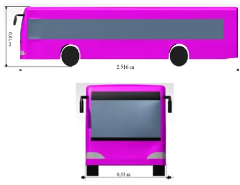
In this study, a 1/5 scale city bus was modeled and aero-dynamic analysis was performed with ANSYS Fluent®. The 1/5 scale model of the city bus was created with the CATIA and the front and side views of the bus dimen-sions are given in Figure 1. Drag coefficient of the bus without side mirror was calculated to examine the effects of the side mirrors and cameras on the aerodynamic drag.
Fig. 1. Front and side views of the bus
During the CFD analysis of the model bus, a control vol-ume was created by using the appropriate blockage ratio for a continuous set of streamlines on solution domain boundaries. The blockage ratio is defined as the frontal area of the object/cross-section of the wind tunnel. The minimum blockage ratio in wind-tunnel testing is re-quired to be 4% [9]. In this study, the blocking ratio was used as 5% and the dimensions of the cross-section of the control volume perpendicular to the flow are deter-mined as 2.4 m x 2.8 m. The distance of the front of the vehicle from the control volume is 0.75 times the length of the vehicle, and the distance of the rear is 1.5 times the length of the vehicle.
Fig. 2. The mesh structure of solution domain As seen in Figure 2, tetrahedral mesh structure is used on the solution domain. Since the speed changes due to viscous effects on the surface of the bus will be high, the inflation layers are created on whole surface of the body. The mesh structure is divided into small element sizes by utilizing the body sizing control. In the investigation of mesh independence, inflation layers has been kept con-stant and CFD analyses have been conducted with changing the mesh element size of solution domain and surface of the vehicle body.
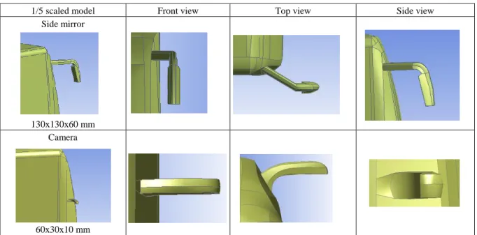
140 Table 1. Side mirror and proposed camera housing
1/5 scaled model Front view Top view Side view
Side mirror
130x130x60 mm Camera
60x30x10 mm
In Table 1. side mirror and proposed camera housing are indicated. Dimensions of the side mirror and proposed camera housing of 1/5 scaled bus are 130x130x60 mm and 60x30x10 mm respectively. Dimensions of the camera, used as reference for housing modeling, are approximately 35 mm length and diameter of 25 mm. A camera housing are designed and positioned to fit the bus regarding the camera dimensions.
2.1 Turbulence Model
The turbulence model has been chosen based on the re-sults of a published study [10]. In the published study, the drag coefficient for Ford K passenger car obtained from wind tunnel test were compared with the results calculated
by realizable k and Reynolds Stress (RSM) turbulence
models. It is stated that the drag coefficient obtained from the RSM turbulence model approaches shows excellent agreement with the experimental results. In this study RSM turbulence model was chosen for use in CFD analysis.
The ANSYS Fluent® generally performs turbulent flow analysis with RANS based turbulence models. In RANS turbulence models, continuity and momentum equations are rearranged by Reynolds decomposition and time averages, and this method shows statistical properties. In derivation of RANS equations, firstly, terms of turbulent flow quantities such as u, v, w and p were decomposed average and fluctuating components. For example, instantaneous u
velocity is decomposed in the RANS model as 𝑢 = 𝑢̅ + 𝑢′.
Terms of 𝑢̅ and 𝑢̅ shows the mean velocity and
fluctua-tions of instantaneous u velocity within timet. Then the
time average of turbulent flow quantities is taken. As a re-sult of these operations, continuity equation and general momentum equations for incompressible flows may be stated as respectively;
, 0
i j
u (1)
1 1
j i
i i
j i
j
j i j
i j
u u
u u p x x
u
t x x x
u u
(2)
The term u ui j given in the Equation (2) shows the
stresses caused by turbulence and is called as Reynolds stress tensor. RANS based turbulence models are solved through the Eddy viscosity concept or using transport equa-tion models. Disregarding the isotropic eddy-viscosity hy-pothesis, the RSM closes the Reynolds-averaged Navier Stokes equations by solving transport equations for the Reynolds stresses, together with an equation for the dissipa-tion rate. RSM method used in this study is the second or-der differential equation model with 7 equations that is, the transport equations are solved in 3D [11]. In second order models, Reynolds stresses and turbulence flows (second order moments) are calculated by using conservation equa-tions directly instead of Boussinesq approach.
Figure 3 shows the sub-options and equation constants selected in the RSM turbulence method. In the analysis, linear pressure-strain, standard wall functions and standard equation constants given in Fluent® program were used.
141 Fig. 3. Sub-options and constants of RSM turbulence model
2.2 Boundary Conditions
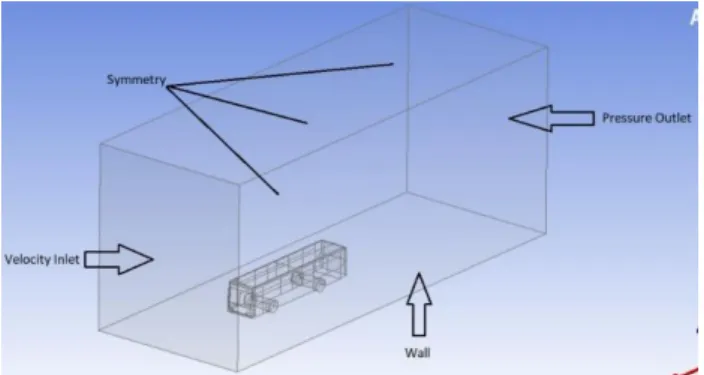
Figure 4 indicates boundary conditions of the solution domain. The wall boundary condition is defined for the bottom surface of solution domain because of that the vehi-cle is practically on the road. The symmetry condition is used to disregard shear stresses on the right, left and top sides of the solution domain. The wall boundary condition is defined on the entire surface of the bus.
Fig. 4. Solution domain and boundary conditions 2.3. Mesh Independency and Mesh Quality
Sufficient number of mesh is required for the accuracy and stability of the analysis. While insufficient number of mesh usage causes errors in analysis, the use of more than optimum level causes unnecessary process time. For this reason, mesh independence of the solution needs to be in-vestigated. In this study, using the tetrahedral mesh struc-ture, the mesh independence of the analysis was investigat-ed with 10 m/s fluid velocity for bus model without side
view mirrors. Table 2 gives the drag coefficients calculated for the nodes and element quantities used in all analyses. It is seen that the mesh structure with 1.3 million elements is sufficient. In the analyses, where the Fluent solver is used, the mesh quality values of skewness, aspect ratio, and growth rate might be maximum as 0.9, 40, and 1.2 for the tetrahedral mesh. In this study, these mesh quality limita-tions are regarded.
Table 2. Calculated CD values depending on number of nodes and elements
Node Element Drag coefficient, CD
130397 575098 0,54
194418 839638 0,52
261519 1090081 0,51
299905 1300400 0,508
326280 1441804 0,508
2.4. Reynolds Independency
After the mesh independence obtained as a result of the calculations, Reynolds independence should be investigated. While performing the process, the optimum mesh element quantity is used and inlet velocity is increased until the drag
coefficient is fixed. The CD coefficients were determined by
increasing the inlet velocity with 10 m/s intervals starting from 10 m/s. After 90 m/s inlet velocity there was no
signif-icant increase in CD coefficient and this speed was found
suitable for all analysis. Table 3 indicates the CD
coeffi-cients of bus without side-view mirror according to the ve-locity.
Table 3. Calculated CD values depending on velocity
Inlet velocity Drag coefficient, CD
10 0,508
30 0,506
50 0,504
70 0,5
90 0,503
100 0,503
3. Results and Discussions
In Figure 5, the velocity contours in the direction of air-flow was shown on a sectional area that longitudinally di-vides control volume into equal. In Figure 5, the analysis was carried out for the 10 m/s inlet velocity and it can be seen that the fluid velocity at the boundaries of the control volume except the bottom is the same as the free stream velocity. As a result, it is understood that the created control volume dimensions are adequate to perform the analysis correctly.
142 Fig. 5. Velocity contours on flow direction
Aerodynamic analysis was carried out for bus models without mirror, with mirror and camera by using the 1.3 M element number and 90 m/s inlet velocity. Drag coefficients due to pressure loss and viscous effects are given in Table 4. Drag coefficients were calculated as 0.503, 0.539 and 0.521 for bus models without mirror, with mirror and camera, respectively. Because of the large cross-sectional area of the side mirrors, high pressure areas were formed on the mir-rors housing, it was observed that the wind resistance coef-ficients increased due to both pressure difference and vis-cous effects. Drag coefficient of the bus model with camera decreased by 3.4 % compared to the bus model with side view mirror model.
Table 4. Drag Coefficients
Pressure Viscous CD
without mirror 0,4707 0,0330 0,503
with mirror 0,5116 0,0288 0,539
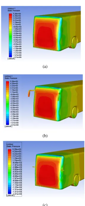
with camera 0,4953 0,0265 0,521 In Figure 6, the pressure distributions on the bus without side mirrors, with side mirrors and cameras are indicted. High-pressure regions appear on the interior of the side mirrors. Low-pressure distribution is observed on camera housing.
4. Conclusions
In this study, the drag coefficient of a bus with classic side mirror was found to be 6.6% higher than the bus without mir-ror it was determined that using a camera instead of the side mirror decreased the friction coefficient by 3.45%. The side mirrors have been increased the drag coefficient of the bus by 0.036. The cameras have been increased by 0.018. As a result, a half gain was achieved in the drag coefficient. The effect of the side mirrors on the bus drag coefficient is a non-negligible amount, and significantly increases fuel consumption. Using camera systems to be placed in smaller volumes instead of side view mirrors reduces the drag coefficient of the bus, resulting in a significant reduction in fuel consumption. Drag coefficient can be further reduced by investigating on the geometric
struc-ture of the camera housing or the position of the camera.
(a)
(b)
(c)
Fig. 6. Pressure distributions on the bus model (a) without mir-ror, (b) with mirmir-ror, (c) camera
References
[1] Wang, J., Bartow, W., Moreyra, A., Woyczynski, G., Lefebvre, A., Carrington, E., & Zha, G. (2014). Low drag au-tomotive mirrors using passive jet flow control. SAE Interna-tional Journal of Passenger Cars-Mechanical Systems, 7(2014-01-0584), 538-549.
[2] Gan, J., Li, L., Zha, G., & Czlapinski, C. (2017). Truck rear view mirror drag reduction using passive jet boat tail flow control. SAE Technical Paper (No. 2017-01-1538).
[3] Roy, J. V., Kumar, T. S., Kumar, R. A., Jeeva, S., & Kumar, V. V. (2018). Aerodynamic design improvement for an
inter-143 city bus. International Research Journal of Automotive
Tech-nology, 1(4), 85-90.
[4] Ipci D., Yılmaz E., Aysal F.E., Solmaz H. (2015). Numerical investigation on the flow pattern around a land vehicle. Elec-tronic Journal of Machine Technologies 12(2), 51-64. [5] Gebel M.E., Önaldı S., Korkmaz S., Osmanoğlu S., Özçelik
B., Ermurat M., İmal M. (2018). Experimental and numerical investigation of aerodynamic properties of an electrical vehi-cle. 9th International Automotive Technologies Congress, OTEKON.
[6] J Howell, J., Windsor, S., and Le Good, G. (2006). A Novel test rig for the aerodynamic development of a door mirror. SAE Technical Paper (No. 2006-01-0340).
[7] Hirose, K., Nakagawa, R., Ura, Y., Kawamata, H., Tanaka, H., & Oshima, M. (2015). Application of prediction formulas to aerodynamic drag reduction of door mirrors. SAE Tech-nical Paper (No. 2015-01-1528).
[8] Buscariolo, F. F., & Rosilho, V. (2013). Comparative CFD study of outside rearview mirror removal and outside rear-view cameras proposals on a current production car. SAE Technical Paper (No. 2013-36-0298).
[9] Katz, J. (2016). Automotive aerodynamics. John Wiley & Sons.
[10]Lanfrit M. (2005). Best practice guidelines for handling Au-tomotive External Aerodynamics with FLUENT. Darmstadt: Fluent Deutschland GmbH.
[11]ANSYS FLUENT 12.0 Theory Guide - 4.9 Reynolds Stress Model.