Review Article
Sequential Monte Carlo Localization Methods in Mobile
Wireless Sensor Networks: A Review
Ammar M. A. Abu Znaid,
1Mohd. Yamani Idna Idris,
1Ainuddin Wahid Abdul Wahab,
1Liana Khamis Qabajeh,
2and Omar Adil Mahdi
11Faculty of Computer Science and Information Technology, University of Malaya, 50603 Lembah Pantai, Kuala Lumpur, Malaysia 2Computer Engineering and Science Department, Information Technology and Computer Engineering Faculty,
Palestine Polytechnic University, Wadi-Alhariya St, P.O. Box 198, Hebron, State of Palestine
Correspondence should be addressed to Mohd. Yamani Idna Idris; [email protected]
Received 13 December 2016; Accepted 13 March 2017; Published 3 April 2017 Academic Editor: Mohannad Al-Durgham
Copyright © 2017 Ammar M. A. Abu Znaid et al. This is an open access article distributed under the Creative Commons Attribution License, which permits unrestricted use, distribution, and reproduction in any medium, provided the original work is properly cited.
The advancement of digital technology has increased the deployment of wireless sensor networks (WSNs) in our daily life. However, locating sensor nodes is a challenging task in WSNs. Sensing data without an accurate location is worthless, especially in critical applications. The pioneering technique in range-free localization schemes is a sequential Monte Carlo (SMC) method, which utilizes network connectivity to estimate sensor location without additional hardware. This study presents a comprehensive survey of state-of-the-art SMC localization schemes. We present the schemes as a thematic taxonomy of localization operation in SMC. Moreover, the critical characteristics of each existing scheme are analyzed to identify its advantages and disadvantages. The similarities and differences of each scheme are investigated on the basis of significant parameters, namely, localization accuracy, computational cost, communication cost, and number of samples. We discuss the challenges and direction of the future research work for each parameter.
1. Introduction
The digital world is becoming increasingly important in our daily lives with the heavy utilization of numerous small, cheap devices called sensor nodes. These sensor devices can be controlled and can communicate and cooperate remotely to investigate far and hazardous areas [1–4]. Sensor nodes are utilized in different fields, such as the Internet of Things [5, 6], health care [7], zoo monitoring [8], underwater exploration [9], intelligent city [10, 11], military applications [12], routing optimization [13], and dynamic mapping [14, 15].
The localization schemes in wireless sensor networks (WSNs) can be classified into two types, namely, static and mobile networks [16]. A static network is constructed with stationary sensor nodes; the sensors are deployed randomly or on the basis of a previous plan. By contrast, the sensor nodes in a mobile network are flexible to maximize their benefits in improving WSNs coverage and power consump-tion and in discovering other areas with a limited number of sensors [17].
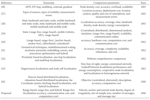
Generally, the localization schemes of a mobile sensor are classified as range-based and range-free schemes [18, 19]. However, in this work, we classified the localization schemes into three groups, namely, range-based, range-free, and hybrid schemes. The range-based scheme uses additional hardware such as antenna to estimate the location of a blind node (i.e., a node without location information), whereas the range-free scheme uses network connectivity. The hybrid scheme is a combination of the range-free scheme for noise cases and the range-based scheme for stabile cases. In all the aforementioned schemes, anchor nodes (i.e., nodes with location information) broadcast their location information per time slot to assist blind nodes in estimating their location. Range-free localization schemes are classified into four categories, namely, hop count, fingerprint algorithm, Monte Carlo scheme, and hybrid schemes (SMC and hop distance). The hop count estimates the location of a blind node through an average of hop distance. Hence, each node maintains the minimum hop number of the anchor node in the network.
In the fingerprint algorithm, the location of a blind node is estimated in two stages. The first stage involves the construction of an offline database by measuring the signal strength in the deployment area, and the second stage involves the real-time estimation of the location of a blind node by matching the signal strength of this blind node with the offline database. The Monte Carlo scheme uses the prob-ability distribution function (PDF) to estimate the location of a blind node [19]. The hybrid schemes (SMC and hop distance) advance localization accuracy by utilizing the DV-hop (distance vector-DV-hop) technique on MCL (Monte Carlo localization).
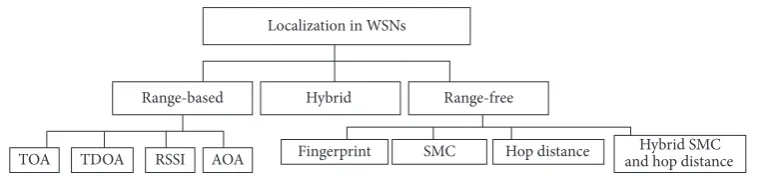
A majority of range-free schemes use the sequential Monte Carlo (SMC) technique to estimate the location of blind nodes in dynamic systems within three steps, namely, initial, sample, and filter stages [20, 21]. The location of mobile sensors is an important parameter in WSNs. Thus, a high level of localization accuracy can improve the confidence and quality of sensing data. In the present study, we classified the performance of SMC schemes according to three categories, namely, localization accuracy, computational cost, and com-munication cost.
Localization accuracy is measured with the variance of the Euclidean distance between the estimated location and the real location [11]. The localization accuracy in SMC schemes is mostly affected by two parameters, namely, the density of anchor nodes and number of samples [22–24]. Hence, a large number of anchor nodes can improve local-ization accuracy by broadcasting rich location information in the area. Moreover, a sufficient number of valid samples can improve localization accuracy. However, the performance of SMC schemes is extremely dependent on the distribution function of previous samples.
The computational cost to generate a sufficient valid sam-ple can be measured with the number of iterations required to find a sufficient valid sample. SMC requires a sequential repetition of sample and filter steps until a sufficient valid sample is obtained. The efficiency of the samples is also affected by the bounded sample area and sample evaluation [25].
The communication cost in range-free localization schemes can be determined with the number of messages that are sent during the localization process [26]. Consequently, the accuracy in range-free schemes is highly dependent on the density of anchor nodes and normal nodes (node’s new location in the last time slot), which can increase the number of messages sent. Moreover, the size of messages affects communication cost.
The following are the contributions of the present study: a comparison of existing surveys on WSNs localization, a classification of state-of-the-art SMC schemes and a thematic taxonomy, a comprehensive survey of state-of-the-art local-ization operation parameters, a discussion of critical aspects, and the identification of challenges and open issues.
This paper consists of eight sections organized as follows. Section 2 presents the comparison of current surveys on sensor localization. Section 3 defines the thematic taxonomy of existing localization schemes. Section 4 explains the
elementary approach related to SMC and the evaluation parameters for the localization process. Section 5 reviews the state-of-the-art SMC schemes by discussing their advantages and disadvantages. Section 6 presents a comparison of state-of-the-art SMC techniques. Section 7 presents the discussion and future works. Finally, Section 8 concludes the review.
2. Comparison of Surveys on
WSNs Localization
Localization problems have been studied in various WSNs schemes; a survey of these schemes can be found in [18, 27, 31, 32]. The present study presents a comprehensive review of the localization problem in mobile WSNs. However, to highlight and distinguish our contribution from other surveys, we summarized and compared the existing surveys on localization problems in WSNs, as shown in Table 1.
In general, previous schemes maintain static networks, whereas current schemes maintain mobile networks. How-ever, the localization schemes in both networks can be classified as range-based and range-free [37]. The survey in [28] classified the state of sensors into four types, namely, static landmark node and static node, mobile landmark node and static node, static landmark node and mobile node, and mobile landmark node and mobile node.
The survey of range-free schemes in [18] classified these schemes into the following categories: APIT, DV-hop, multihop, centroid, and gradient. Another survey classified range-free localization schemes in emerging applications (cyber physical systems and cyber transportation systems) into proximity-based localization, one-hop localization, and multihop localization. Moreover, range-based schemes were classified in [16] into beacon-based distributed localization, relaxation-based distributed algorithm, coordinate system stitching-based localization, and hybrid localization. Beacon-based distributed localization can be further classified into three categories, namely, diffusion, bounded box, and gradi-ent.
The survey in [29] classified mobile sensor networks in disaster scenarios, in which mobile nodes aid in the search for disaster locations. The localization schemes in static networks are classified as range-free and range-based schemes, whereas those in mobile networks are classified as robotic, MCL, and range-based schemes. Another survey on harsh environments [30] classified localization schemes into range-based and range-free, anchor-based and anchor-free, and distributed and centralized schemes.
Table 1: Previous survey of wireless sensor localization.
Reference Taxonomy Comparison parameters Years
[18] APIT, DV-hop, multihop, centroid, gradient Node density, cost, accuracy, overhead, scalability 2015
[27] Types of sensors, types of mobility, measurement
errors
Location accuracy, deployment cost, location context, quality and cost of smartphone, and
measurement errors
2015
[28]
Static landmark and static node, mobile landmark and static node, static landmark and mobile node,
mobile landmark and mobile node
Localization accuracy, coverage, time, landmark
density, node density, energy consumption 2013
[29] Static (range-free, range-based), mobile (robotic,
MCL, range-based)
(Centralized, distributed), dimensional analysis, simulator, (range-free, range-based), scalability,
communication radius
2013
[30] (range-based, range-free), (anchor-based,anchor-free), (distributed, centralized) accuracy, hardware cost, computation cost, andcommunication cost 2012
[31]
Geometrical techniques, multidimensional scaling, stochastic proximity embedding convex, and
nonconvex optimization and hybrid
Accuracy, coverage, complexity, scalability,
robustness, and cost 2012
[32] Proximity-based localization, one-hop localization
and multihop localization Without comprehensive comparison 2012
[33] Target/source localization and node self-localization
Non-line-of-sight, energy-constrained network, tradeoff between localization performance and energy consumption, cooperative node localization,
and localization in heterogeneous network
2012
[16]
Beacon-based distributed localization, relaxation-based distributed localization, the Coordinate system stitching-based localization, and
hybrid localization
Objective (centralized, distrusted), description,
accuracy, computation cost 2010
Proposed
Range-based, range-free, and hybrid. Range-free (localization accuracy, communication cost, and
computation cost)
Velocity, anchor and normal node density, degree of irregularity, size of sample area, number of messages,
and message size
2016
survey reviewed the localization challenges in non-line-of-sight node selection, optimizing the tradeoff between energy depletion performance, cooperative nodes, and localization in a heterogeneous radio range.
The present survey investigates the state-of-the-art local-ization schemes in mobile WSNs in microscopic classifica-tion. The schemes are categorized as range-based, range-free, and hybrid. The range-free scheme is further subcategorized into fingerprint, Monte Carlo, hop distances, and hybrid (i.e., SMC and hop distance). Furthermore, we classify the SMC scheme according to its main operational parameters, namely, localization accuracy, communication cost, and com-putation cost, in microscopic classification. The comparison of the localization schemes assists network end users and administrators in tracking and identifying the location of areas under investigation. Thus, appropriate schemes are selected to localize mobile WSNs. Throughout this study, we further discuss the challenges and open issues related to each location parameter.
3. Localization Scheme Classification
Estimating the location of mobile sensors is a challenging task in WSNs because of the frequent changes in the location of mobile nodes per time slot, the whole topology, and con-nectivity of networks. Additionally, the sensor node’s
hard-ware limitations, such as limited power sources, memory, processor unit, and communication range, further compli-cate the estimation process [38]. Therefore, WSNs need a smart and robust technology to estimate sensor location. We classified localization schemes into three categories, namely, range-based, range-free, and hybrid; the SMC in range-free schemes was classified on the basis of localization accuracy, communication cost, and computation cost, as shown in Figure 1.
3.1. Range-Based Localization. In range-based schemes, the
blind node finds its location using its absolute distance from the anchor nodes. Range-based schemes use different types of hardware to calculate distance, such as time of arrival (ToA). ToA measures the distance between the time of arrival and the time of departure between nodes. Then, light speed is used to calculate the distance between nodes on the basis of a speed equation. However, ToA needs additional hardware to synchronize the transmission times between sensor nodes. The time synchronization increases the traffic in networks and delays the localization process [39].
Localization in WSNs
Range-based Range-free
AOA RSSI TDOA
TOA Fingerprint SMC Hop distance
Hybrid
[image:4.600.110.489.70.158.2]Hybrid SMC and hop distance
Figure 1: Taxonomy of localization schemes in mobile WSNs, including range-free and sequential Monte Carlo schemes.
also used to calculate blind node location. In AoA, the sensor node uses antennas to measure the angle between neighbors [41].
The received signal strength indicator (RSSI) measures the distance according to the difference in signal strengths [42]. The RSSI assumes that signal strength degrades over distance; this characteristic is used to measure distance without additional hardware. However, signal strength is affected by noise, such as physical phenomena and weather conditions; these distortions reduce the accuracy of distance measurement.
The global positioning system (GPS) is typically used to localize objects in outdoor applications. However, GPS is inapplicable to indoor applications because GPS requires the lines-of-sight of at least three satellite signals at the same time to determine the location of an object [43]. Moreover, GPS signals are affected by obstacles, walls, and physical phenomena. The other limitations of GPS include high power consumption, high cost, and large size.
3.2. Range-Free Localization. Range-free schemes estimate
blind node location through network connectivity without additional hardware. Thus, the blind node requires the following: information about nodes that are within its radio range, the location estimation of nodes, and the ideal radio range of each sensor. The anchor nodes in range-free schemes broadcast their locations at each time slot to help the blind node in estimating its location. Generally, the blind node needs at least three anchor node locations in the neighbor-hood to estimate its location. Range-free schemes are more cost-effective than range-based schemes. Range-free schemes can be classified into the following types: hop distance, fingerprint, SMC, and hybrid schemes utilizing SMC and hop distance.
Hop Distance. Hop distance uses the average hop to
esti-mate the distance between anchor nodes. The localization process in DV-hop follows three steps, namely, location broadcast, distance calculation, and location estimation [44]. In location broadcast, the anchor node broadcasts its location information and initializes the hop count to zero among its neighbors. The receiver node keeps the minimum hop count for each anchor node and disregards the large hop count from the same anchor nodes. Then, the receiver increases the hop count by one and sends it to the neighbors. Hence, each node has a record of the minimum hop count of all anchor nodes. In distance calculation, the node calculates the
average distance with each anchor node over the hop count of all anchor nodes. In location estimation, the blind node calculates its location by interlocking the matrixes of anchor node location and the matrixes of distance with anchor nodes [45]. The disadvantage of hop distance is that it requires a uniform distribution of anchor nodes in the whole network to achieve high accuracy. Consequently, DV-hop is limited to specific applications.
Fingerprint. The fingerprint localization approach estimates
blind node location in two steps, namely, creation of an offline database and online location estimation. The offline database is constructed from signal characteristics (called fingerprints) and the location recorded from the whole part of the area of interest. Then, location is estimated for the mobile user by matching the signal fingerprint from the user with that in the database server. Once the signal fingerprint matches that in the database server, the estimated location is sent back to the user. The main drawback of the fingerprint localization approach is the creation and updating of the database. Creating the database requires some expert personnel to collect fingerprints from areas of interest; updating the offline database is a time-consuming task when changes, such as the addition or removal of a new access point in the area of interest, are made in the environment. Moreover, mobile sensors can share similar fingerprints that degrade accuracy and promote ambiguity. This drawback of the fingerprint localization approach requires a qualified engineer who would measure signal strength [46].
Sequential Monte Carlo (SMC). Mobile sensors change their
locations frequently over time. Hence, finding their current locations requires relocalization at each time slot. SMC is an efficient method for a dynamic system; SMC employs the PDF in the previous time slot and observes it at the current time to estimate the current location by using a weighted particle filter [47].
SMC makes the following two assumptions: (1) time is divided into discrete time units and (2) enough samples are required at each time slot. The SMC scheme estimates blind node location in a distributed manner on the basis of the connectivity information “who is within the communication range of whom” [48].
sample stage, the blind node draws samples in the current time slot on the basis of the samples from the previous time slot bounded by a maximum velocity. Hence, the node generates samples through the following transition equation:
𝑝 (𝑆𝑡| 𝑆𝑡−1) =
{ { {
1
𝜋Vmax2 if𝑑 (𝑆𝑡| 𝑆𝑡−1) ≤Vmax,
0 if𝑑 (𝑆𝑡| 𝑆𝑡−1) >Vmax, (1)
whereVmaxis the node maximum velocity and𝑑(𝑆𝑡| 𝑆𝑡−1)is the distance of the sample location between the current time and the previous time.
In the filter stage, the samples are weighted according to the anchor node constraint in the current time. Each valid sample must be within one or two hops of the three anchor node constraints. Otherwise, the sample is filtered out. SMC repeats the sample and filter stages sequentially until sufficient valid samples are discovered.
Algorithm 1(phase of SMC localization algorithm).
(1)Phase One. Initial phase
(2) Generate samplesSrandomly from the whole area.
(3)Phase Two. Generating samples
(4) Sample set𝐶𝑡= {}
(5) For each sample S in previous time(𝑙𝑡−1), generate a new sample according to
(6) Sample𝑙(𝑖)𝑡 ∼ 𝑝(𝑙𝑡| 𝑙(𝑖)𝑡−1)
(7) Weight of𝑙(𝑖)𝑡 as ̌𝑤𝑡(𝑖)= 𝑝(𝑜𝑡| 𝑙𝑡(𝑖)) (8)𝐶𝑡=𝐶𝑡∪ {(𝑙𝑡(𝑖), ̌𝑤(𝑖)𝑡 )}
(9)Phase Three. Filtering
(10)𝐶𝑡= {(𝑙𝑡(𝑖), ̌𝑤(𝑖)𝑡 ) | (𝑙(𝑖)𝑡 , ̌𝑤𝑡(𝑖)) ∈ 𝐶𝑡 and ̌𝑤𝑡(𝑖)> 0} (11) Normalize the weight of valid samples𝑤𝑖𝑡= ̌𝑤𝑡𝑖/ ∑𝑁𝑖=1 ̌𝑤𝑖𝑡 (12) Set the average of the samples as the blind node
location.
(𝑖)is the index of samples,𝑜is observation at current time, and𝐶is the sample set.
The filtration efficiency of the SMC localization scheme is mostly affected by anchor node density in the neighborhood. For example, under low anchor node density, a blind node is not always able to identify three anchor nodes in the first hop and second hop, especially when the sensor moves with high velocity; this process occurs because the first hop neighbors that communicate with radio range𝑅are unable to identify within its range the second hop sensor that communicates with radio range2𝑅.
Hybrid Schemes (SMC and Hop Distance). The multihop
version of Monte Carlo localization (MMCL) [49] improves localization accuracy and reduces the dependence on anchor nodes by utilizing the DV-hop technique on MCL. MMCL measures the average hop distance between anchor nodes and then uses MCL to estimate blind node location. The DV-hop schemes have two drawbacks. First, these schemes need
a uniform distribution of anchors to achieve high accuracy. Second, broadcasting the location information of anchor nodes to multiple hops increases the communication cost.
The hybrid scheme presented in HMCL [50] utilizes hop distance and the SMC technique to improve localization accuracy. The sample area is constructed over the intersection area between anchor boxes. The anchor boxes are formed over the midpoint between anchor nodes. This scheme can reduce the size of a sample area and improve the localization accuracy through a virtual anchor node. The disadvantage of this scheme is that additional computation is required to estimate the distance and angle between the anchor node and the virtual anchor node.
3.3. Hybrid Localization Scheme (Free and
Range-Based). The combination of range-based and range-free
schemes can improve localization accuracy in WSNs. The RSSI is a simple range-based scheme that measures the dis-tance between two nodes by evaluating the signal strength indicator without additional hardware. Signal strength declines over distance. Hence, the RSSI utilizes this phenom-enon to measure distance in the localization process. Con-sequently, communication and computational costs are reduced in the SMC technique [51].
The based MCL (RMCL) scheme combines range-based and range-free schemes during the localization process to overcome the high radio measurement error that reduces localization accuracy in range-based schemes. RMCL is a hop distance scheme that maintains the hop count and measurement range at a minimum for each anchor node. However, broadcasting the minimum measurement range for each anchor node increases the communication cost in this hop distance method. Moreover, computing the weights in RMCL is a complex task [52, 53].
The Monte Carlo box localization algorithm based on RSSI (MCBBR) [54] uses a reference genetic algorithm (linear crossing and rectangular crossing) to enhance the localization accuracy of the RMCL scheme and RSSI obser-vation to optimize the sample area. In MCBBR, the localiza-tion accuracy is determined with the following four steps, namely, constructing the sampling box, establishing the sample number, optimizing the sample, and estimating the location. The real implementation of RMCL [52, 55] shows that the RSSI improves the accuracy of personal location inside an operation environment. Another improvement of RMCL [53] involves the use of SMC to increase localization accuracy when the range measurement has high variation; this improved scheme also utilizes range measurement to reduce computational costs.
SMC
Accuracy Computation cost Communication cost
Velocity
Anchor node density
Normal node density
Sample area size
Number of samples
Number of messages
[image:6.600.154.444.73.197.2]Message size
Figure 2: Evaluation parameter in SMC localization scheme.
the sample stage because the log-normal model is embedded with complex equations [52].
In real-world applications, range measurement is affected by path loss, fading, and shadowing phenomena. Hence, radio range can be protected by environmental factors, such as obstacles, rain, wind, and humidity; it can also be affected by the indoor environment. However, the range noise of the RSSI minimizes localization accuracy. Other studies [21, 56] presented the SMC scheme to enhance the localization accuracy associated with the noise measurement amount.
4. Evaluation Parameters in SMC Localization
The SMC localization in mobile WSNs is mainly evaluated according to localization accuracy, computational cost, and communication cost, as presented in Figure 2.
4.1. Localization Accuracy. Localization accuracy is the most
important parameter of WSNs. A high level of localization accuracy can help decision-makers to identify the precise location and coverage area of data. Localization accuracy can be measured with the variance between a real location and an estimated location, as shown in (2). For simplicity during the simulation test, the SMC technique is employed with the assumption that the anchor nodes know their real locations without error at all times.
Localization accuracy= 1
𝑛
𝑛
∑
𝑖=1𝑒𝑖
− 𝑙𝑖, (2)
where𝑛is the number of sensor nodes,𝑒𝑖 is the estimated location, and𝑙𝑖is the real location. The error in the equation is given in terms of radio range and is thus divided by the sensor radio range.
The localization error in the initial step is reduced quickly when the new observations arrive. In the stability step, the localization error is maintained at around the same mean error. Thus, the effects of mobility and connectivity are in equilibrium. The localization accuracy of the SMC technique is mostly affected by the movement velocity, anchor node density, normal node density, and degree of irregularity.
The Movement Velocity. The mobility of sensor nodes can
maximize the benefits of WSNs in various aspects. This
mobility allows sensors to communicate with a large number of neighboring anchor nodes. Hence, localization accuracy can be improved with the minimum number of anchor nodes. Mobility also conserves energy and prolongs network lifetime by changing routing paths [57]. Static WSNs use the same routing path, through which messages are sent and received frequently, even though the sensor is near the sink node; this frequency exhausts energy and causes network partition [27, 58, 59]. In real-world applications, the mobility of sensor nodes allows animals to be traced in zoos and patients to be monitored in hospitals, in addition to their other applications. However, this mobility presents an additional challenge in the handshaking case, in which the sensor is outside the neighbors’ range to transmit and receive data [60, 61].
The mobility model is classified into three categories, namely, controlled, predefined (map), and random. The details of these categories are explained in [62]. In most schemes, the SMC technique is used to select a random waypoint model to transmit nodes. The waypoint model is a simple and independent model. Moreover, the sensor node can choose its new direction and velocity randomly without exceeding its maximum velocity [63]. The pause time is set to 0 in most schemes; this zero pause time allows the sensor to move without stopping [64].
The velocity of a sensor node affects localization accuracy differently. A sensor node with a low level velocity achieves the highest localization accuracy because this node is still in the range of the sample from the previous location, which this node reuses to estimate a new location accuracy. A sensor node with a high level velocity can exert a negative effect on localization accuracy if it moves far from the sample in the previous location and becomes unreachable. However, a high velocity guide sensor explores additional areas per time slot.
Anchor Node Density. The localization accuracy of all schemes
area. A narrow sample area requires additional time for blind nodes to generate proper samples. The SMC technique addresses these drawbacks by employing a high number of anchor nodes in the region to maintain a high localization accuracy. In the literature, some schemes such as Monte Carlo localization (MCL) [26] and Monte Carlo localization boxed (MCB) [65] are fully dependent on the information of anchor node location, whereas others combine both anchor and normal nodes in the localization process.
Normal Node Density. The information on normal node
location can be used during the positioning process to enhance localization accuracy and reduce the dependence on anchor nodes. The utilization of normal nodes can enhance localization accuracy in two ways. First, normal nodes retransmit the location information of the anchor node to its neighbors. Second, the location information of the normal nodes is used in the localization process; using this information in the sample step narrows the sample area and filters out the invalid samples in the filter step. However, the use of normal node location in the localization process is susceptible to error and significant communication cost in the network. Therefore, this localization process requires a precise and lightweight method.
Degree of Irregularity. The variation of the radio range
between sensors leads to communication failure, which degrades the localization accuracy of WSNs [66, 67]. For simplicity, radio range is assumed to be a full circular range in most of previous schemes’ simulation experiments. However, this assumption does not present the actual radio range in real-world applications; in reality, radio range is affected by sensor characteristics, such as antenna direction and sensor power, and by the types of transmission media, such as humidity, temperature, obstacles, and wind speed. These factors can distort radio range at different degrees.
4.2. Computational Cost. Computational cost is quantified
from the iteration to generate enough valid samples in each time slot. The main parameters that affect computational cost are the size of the sample area and the number of samples. The sample and filter stages are repeated until enough valid samples are found; this process is costly because it wastes additional power and delays the localization process.
High velocity and high anchor node density negatively affect sample efficiency in the following ways. A high velocity maximizes the sample area. Thus, the sample generation and filtering steps are repeated several times to draw enough valid samples for a large area. A high anchor node density narrows the sample area. Hence, the generation and filtering steps are repeated to generate dissimilar samples.
Sample Area Size. In the literature, various strategies are used
to draw samples. An example is the random generation of a sample over a previous sample bounded by a circle with a radius equal to the maximum velocity and anchor node bounded box. However, the shape of the sample area is irregular and is mostly affected by the number of anchor nodes in the neighborhood.
Number of Samples. The main idea of the SMC technique is
to estimate the location of blind nodes by averaging the weighted samples (or particles). Therefore, the number of valid samples is an important parameter in localization accuracy. A large number of samples can slow down the local-ization process by repeating the generation and evaluation steps. Thus, a typical maximum number of samples is set to 50 [26].
The size of the sample area depends on the anchor node density in the first hop and second hop and on maximum velocity. A large number of anchor nodes in the neigh-borhood equates to a narrow sample area, and vice versa. Drawing a large number of samples in a narrow region is a critical issue because an additional calculation must be performed to remove redundant and closed samples. A large number of samples are required to cover a large sample area. Therefore, a constant number of samples do not represent a sufficient solution for all sizes of sample areas.
The simulation results for different schemes are presented in Table 3; 50 samples are enough to estimate an accurate location. Accordingly, most of the studies in the literature used 50 samples as the maximum number of samples, whereas other studies used an adaptive approach based on the sample area to set the number of samples. Nevertheless, the relation between the number of samples and the sample area is a challenging issue in WSNs.
In the SMC method, drawing valid samples involves the following two steps: (1) drawing candidate samples and (2) evaluating candidate samples. Drawing candidate samples is more costly than evaluating them [68]. Typically, sample efficiency is affected by the number of valid samples and the bounded area of the samples. Hence, a direct relationship exists between the number of samples and the sample area.
Sample evaluation is a measurement of the distance between two points or a comparison between the distance and its predefined value (the communication radio rangeR). The operation cost for measuring the distance between two points is approximately 100 times that for comparing distance and its predefined value, as shown in [68], because the sample generation is repeated until the sample overcomes the anchor node communication radio range.
4.3. Communication Cost. The main purpose of the
range-free localization scheme is to reduce the dependency on hard-ware by utilizing network connectivity during the estimation of blind node location. The estimation process requires net-work connectivity to broadcast messages from sensor nodes. Therefore, communication cost is computed with the number of messages broadcasted during the localization process [26]. The number of messages is affected by the number of anchor nodes and normal nodes used in the localization process. The size of the message also affects communication cost.
Number of Messages. In the SMC method, the anchor nodes
because blind nodes need enough location information to estimate their location. However, a large number of messages may include redundant and closed samples.
The message of location information is categorized into two types according to its content. The first type of mes-sage contains the location coordinate, and the second type contains the sample. The coordinate message commonly defines the exact location of an anchor node on the Cartesian plane; the sample message contains the potential coordinate of the normal node on the Cartesian plane. The sample message can improve localization accuracy, but it increases the communication cost. Nevertheless, the relation between communication cost and localization accuracy is a challeng-ing research area in WSNs.
Message Size. The size of messages transmitted is not fixed
in SMC schemes, as presented in [69]. The anchor message contains the IP header, transmitter ID, anchor location, and number of hops. The standard size of an anchor message is 34 bytes in all schemes. By contrast, the size of a normal node message varies between schemes.
The most vital parameter in the localization process is the localization accuracy. The precise location can increase the confidence on the sensed data and the data originality. The achievement of high localization accuracy is difficult in terms of increasing the computation and communica-tion cost. Thus, the optimal solucommunica-tion should maintain high accuracy with low computation and communication cost. To investigate and highlight this issue, localization schemes in the literature are classified based on these parameters.
5. State-of-the-Art SMC Localization Schemes
Monte Carlo localization (MCL) scheme is pioneered from the SMC schemes; in MCL, time is divided into discrete time slots, the pause time is set to 0, and all sensors move per time slot. After each movement, the node estimates its new location by utilizing the new observation from the anchor nodes in the neighborhood. Therefore, the sample and filter steps are repeated until the sensor collects enough valid samples. The weaknesses of MCL are that it requires high anchor node density to achieve sustainable accuracy and that it uses slow sampling method. The sample and filter steps are repeated up to 1000 times per each sample in MCL.
Dual and mixture MCL schemes improve the accuracy of MCL by inverting the probability function in the dual Monte Carlo scheme during the sample and filter steps [70]. The disadvantages of the dual Monte Carlo scheme are high computational cost and low sample efficiency. The authors slightly improved the sample efficiency in the mixture Monte Carlo scheme by mixing dual Monte Carlo samples and MCL samples. The negative effect of the mixture Monte Carlo scheme is that it has a lower accuracy than the dual Monte Carlo scheme.
The study [71] presented MSL∗and MSL (mobile sensor network localization and static sensor network localization) to improve the accuracy of MCL. The MSL∗ scheme uses the location information of both anchor and normal nodes from the first hop and second hop. The location information
Valid sample area Bounded box
[image:8.600.336.514.67.237.2]Anchor
Figure 3: Bounded area of valid sample area MCB scheme.
contains the samples in the current time slot and their weights. However, broadcasting all node samples increases the communication cost. To reduce the communication cost, MSL is used to broadcast only the location coordinates of the anchor and normal nodes. This strategy reduces the communication cost and localization accuracy.
The MSL∗ scheme adds the additional parameter of maximum velocity(𝛼 = 0.1𝑅)in the sample generation to satisfy static networks. Each normal node sample in MSL∗ has a partial weight in the range of zero to one; the anchor node sample maintains a weight value of 1 at all times. The node keeps its sample on the basis of its weight. Weight is estimated with a power function according to the number of normal nodes in the neighborhood. The node uses the close neighbor’s samples to evaluate its samples. Hence, this node is greatly affected by the number of nodes in the neighborhood. Moreover, the power function in MSL∗entails a higher computational cost than the distance measurement between two point methods. The broadcasting of anchor, normal nodes samples, and their weight in MSL∗ highly increase the communication cost.
In our previous LCC scheme (low communication cost) [72], the communication cost of MSL∗is reduced by selecting the closed normal nodes in the neighborhood instead of selecting all normal nodes as in MSL∗. LCC reduces the communication cost of MSL∗by 18% and maintains the same localization accuracy of MSL∗.
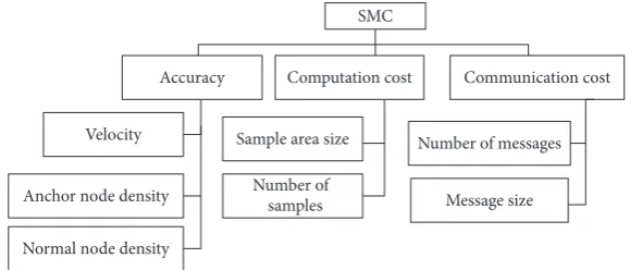
the bounded area. However, such calculation is impossible in sensor nodes. For simplicity, the box surrounding the sample area is used to assess the shape of the sample area, as shown in Figure 3. This implementation improves the sampling efficiency of MCL by 93% and maintains the same accuracy level as that of MCL.
The weighted Monte Carlo localization (WMCL) scheme improves localization accuracy by utilizing the location infor-mation of normal nodes [68], in addition to that of anchor nodes, as in MSL∗. The WMCL scheme reduces the size of the sample area and improves the sample efficiency of MCB by employing the two-hop anchor node neighbors’ negative effect and normal node location information. The estimated location of the normal node contains a fraction of error. To overcome this challenge, the normal nodes utilize the maximum location error in𝑥-axis and𝑦-axis for bounding the sample area. Thus, the sample area in WMCL is bounded by both the anchor node constraints and normal node location information. The normal nodes estimate the errors in both axes. In filtering out the invalid samples efficiently, the weight for the anchor node samples is set to 1 at all times, and the partial weight for the normal node is set in the range of 0 to 1.
The partial weight for the normal node samples in WMCL is calculated as follows. First, the distance between all sensors samples in the neighborhood are estimated. Second, the intersection of the bounded box is utilized to reduce the communication cost of the first step. Finally, the radio range, maximum velocity, and maximum localization error from the previous time are utilized. These processes filter out the invalid samples more efficiently than MSL∗ and quicken the sampling step. Unlike MCB, WMCL reduces the sample area by 78% and improves the sampling efficiency by up to 95%. Moreover, WMCL uses the normal node location information in the sample and filter steps, whereas MCB utilizes only the anchor node location information in the filter step.
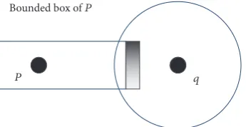
The negative effect of two-hop anchor nodes in the literature is defined as follows: “node𝑥is not within distance
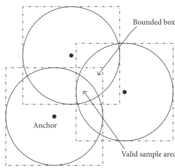
𝑑 of node 𝑦.” Range-free schemes utilize this definition (“node 𝑥 is not within the radio range of 𝑦”) to enhance localization accuracy. The negative effect of two-hop anchor nodes and normal node location information can enhance localization accuracy and sample efficiency by 87% and 95%, respectively, as in WMCL. The shadow area in Figure 4 can be ignored without losing any valid samples; this fact can be explained as follows. 𝑞 is assumed to be the two-hop anchor node for normal node𝑝. Thus, the shadow area does not contain𝑝because, otherwise,𝑞is the one-hop neighbor of node𝑞. The negative effect of two hops is a critical and precise issue. For example, if the distance between node𝑝 and 𝑞is underestimated, then the negative constraints can reduce localization accuracy. On the contrary, if the distance between node𝑝and 𝑞 is overestimated, then the practical location may be lost.
The movement direction of anchor nodes between the previous time slot and the current time slot is used in the con-straint rule-optimized Monte Carlo localization (COMCL) scheme [73]. COMCL utilizes the locations of anchor nodes
P q
[image:9.600.344.517.73.162.2]Bounded box ofP
Figure 4: Improve the size of the bounded box: the shadowed area should be cut.
in the previous and current time slots to track the movement direction of these anchor nodes within the upper and lower bounds. COMCL classifies the location of the anchor nodes per time into two types: moving backward and moving for-ward in time. The location information in COMCL requires the following three steps: (1) construct the anchor node constraint, (2) construct the sample area, and (3) optimize and filter out the invalid samples. COMCL can involve more efficient and faster filtering steps than WMCL; nevertheless, it adds additional calculation. Each anchor node requires calculating the distance with neighbors and comparing the distance with upper and lower bounds to track the movement direction.
The range-based Monte Carlo boxed (RMCB) scheme compares and utilizes both range-based and range-free schemes to answer the question “when does range-based localization work better than range-free localization?” RMCB is suitable for both static and mobile WSNs with a hetero-geneous radio range [74]. RMCB improves the sample area and efficiency in WMCL using a positive anchor node effect behind the negative effect used in WMCL. To ensure the efficiency of RMCB, the authors employed the same hardware devices for both RMCB and WMCL. The result shows that RMCB can improve WMCL in different parameters.
In [69], an improved MCL (IMCL) scheme was used to enhance the localization accuracy in MCL by adding constraints of movement direction in the previous schemes to the anchor and normal nodes. IMCL selects the normal nodes in the first hop’s neighbors whose locations are constructed by the anchor node constraint. Moreover, IMCL employs the circular sector in the localization process to filter out the invalid samples. Each normal node divides the circular range into eight sectors; the longest sample sector is used to filter out the invalid samples. Computing the longest distance of samples and the angle of each sector increases the computational burden in IMCL and can delay the location estimation.
PMCB [75] (permeant Monte Carlo localization Boxed) scheme uses a time series to forecast the position of a blind node in case no anchor nodes exist in the neighborhood. Otherwise, SMC is used to estimate the location. The time series reduces the dependency on the anchor node. However, a recursive step is required to calculate the linear prediction coefficients in each time slot.
constructed with one root and five leaves to optimize the number of neighbors in the network. The orbit coordinates the neighbor’s node constraint within the star graph to improve localization accuracy. The orbit scheme is highly affected by node density. In this scheme, five nodes may not constantly be discovered in the neighborhood [76]. Thus, the accuracy in the low normal nodes density will be reduced.
In [77], a Gaussian process regression was formulated with observations to improve localization accuracy. The observations on noise measurement, localization error, and previous distribution are correlated with the posterior predic-tive statistics. Hence, the posterior predicpredic-tive statistics utilize MCL sampling and Laplace’s method to improve localization accuracy. Laplace’s method requires a complex calculation that is not applicable in thin device like sensor node.
In the sequential Monte Carlo-based localization algo-rithm (SMCLA), each sensor node maintains a table to store the localization parameters: estimated location, velocity, direction, and motion type at the current time slot. The blind node in the initial four steps moves according to the waypoint model. Then, the motion type is estimated by evaluating the velocity, acceleration, and movement direction to generate samples. Hence, the blind node stores the last four pieces of location information in the table with their time stamps. The disadvantage of utilizing the time stamp is that it requires additional hardware for the time synchronization between sensor nodes and the table data protect additional memory size [78].
The variation of radio range is evaluated during the local-ization process in the sequential Monte Carlo locallocal-ization (SMCL) scheme. A perfect circular sector is used to simulate the radio range in most schemes. The radio range in real-world applications is affected by noise, path loss, shadowing, and physical phenomena. Hence, DOI (degree of irregularity) is used to check the variation of the radio range in the SMCL scheme. The updating stage is added to the SMC method to measure the effective factor of each sample in location estimation [79].
In [80], a sample adaptive Monte Carlo localization (SAMCL) algorithm was employed; in SAMCL, the sample area is divided into small bins, and each valid sample is assigned to one bin. The new samples are selected if they are acquired inside an empty bin. Otherwise, they are ignored. Thus, the number of samples is counted by bin numbers. The generated sample can be acquired several times in nonempty sample. Thus it requires repeating the sample generation. Moreover, the size of small bin is a critical issue. The number of bins can be maximized in the large size and minimized in the small size. Thus the localization accuracy will be affected. The uniform sampling Monte Carlo localization (USML) scheme modifies the sampling strategy of SMC by dividing the sample area into small squares; this scheme selects the samples on the basis of their uniform distribution over a small square. The uniform distribution can reduce the time needed to generate random samples over the whole area. However, this uniform distribution does not represent the real state of all systems. Therefore, random generation can improve localization accuracy more efficiently than uniform distribution [81].
Reduce redundant messages and hop distance overhead using the back off-based broadcasting mechanism. This mechanism uses the following assumption in the RSSI: a node that is far from the sender has a signal strength that is too weak to select messages with a signal strength exceeding a predefined threshold [50].
In [82], the location information messages were used to improve failure detection. Generally, sensor nodes in WSNs exchange heartbeat messages to detect neighbors. These messages can be utilized for failure detection during the localization process. Hence, the compound between the localization process and failure detection can reduce the number of exchanged messages in networks.
Localization accuracy can be improved by combining SMC schemes and the genetic algorithm as in Genetic and Weighting Monte Carlo Localization (GWMCL) [83]. Crossover and mutation can be used to draw samples from a virtual anchor node. Hence, linear crossover and rectangular crossover are used to filter out invalid samples on the basis of the distance between the anchor node and the blind node.
The geometry of the intersection points between sensor nodes is used to bound the polygon shape; the shape is used to filter out the invalid samples [34]. However, the shape of the sample area is irregular and depends on the number and location of anchor nodes in the neighborhood. Hence, constructing the polygon is not easy in all cases.
5.1. Schemes Utilizing a Single Anchor Node. A single mobile
anchor node (or online localization) is used to save scarce resources of sensor nodes and improve the localization accuracy of MCL. A blind node requests a location estimation from an anchor node. Thus, the anchor node calculates the location of the blind node and sends it back to the blind node. Mobile-assisted Monte Carlo localization (MA-MCL) scheme uses one anchor node with high resources to localize static blind nodes. The anchor node moves randomly to collect arriver static and leaver static of blind observation. Then, invalid samples are filtered out according to the move-ment direction. After finding the blind node observation, the anchor node calculates the location and sends it back to the blind node [84].
Wireless node-based Monte Carlo localization (WNMCL) is another scheme that utilizes a single anchor node in the localization process. WNMCL divides the sample area into separate clusters. The closed clusters are merged, and the merging is repeated until the number of separate clusters is found. The center of the separate cluster is used as the estimated location of the blind node [85].
A single mobile anchor node with different types of blind node observation, such as connectivity, AoA, ranging, and a mixture of all of these, was utilized to estimate location [35]. The blind node collects at least the connectivity range of the first neighbor and sends this range to the anchor node when it arrives. The localization process occurs in the anchor node side; the location is sent back to the blind node.
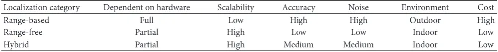
Table 2: Summary of localization schemes categories.
Localization category Dependent on hardware Scalability Accuracy Noise Environment Cost
Range-based Full Low High High Outdoor High
Range-free Partial High Low Low Indoor Low
Hybrid Partial High Medium Medium Indoor Low
improved by securing a single anchor node. Nevertheless, the use of a single mobile node increases the overhead over the beacon node and maximizes the probability of network congestion. Moreover, the noise and overload of a single anchor node range can degrade the localization accuracy of the whole network.
5.2. Schemes Utilizing MCL in Target Tracking. The MCL
scheme enhances target tracking by estimating target loca-tions [86, 87]. The novel Monte Carlo-based tracking (NMCT) scheme utilizes the perpendicular bisector zoning technique and triangulation assumption in the point in trian-gle (PIT) scheme to gather and check the blind nodes within or outside the anchor node triangle [88]. The perpendicular line is used to find the bisector area and check the closeness of the anchor nodes in the neighborhood. Therefore, the possible location of the blind node can be estimated from the anchor node pairs in the PIT and perpendicular bisector line [89]. Therefore, the valid sample area can be bounded, and the invalid samples can be filtered out efficiently. The weakness of NMCT is that it assumes that anchor nodes are static nodes and that normal nodes are mobile nodes.
Oriented tracking-based Monte Carlo localization (OTMCL) scheme utilizes the movement orientation in the sample step to improve MCL accuracy [90]. The angle of the movement sector is calculated on the basis of the elaboration between the locations in the previous and current times. The drawback of OTMCL is the need to constantly find enough valid samples. Thus, OTMCL uses the bounded box in MCB to generate samples.
The binary detection Monte Carlo localization (BD MCL) scheme utilizes the binary assumption in MCL to examine the node with the maximum range or outside range [91]. BD MCL maintains and records the interval time of each mobile sensor in the range. Hence, the mobile sensor with a large time interval has a high weightage sample. The use of the time interval requires the anchor node to synchronize the time between nodes; this synchronization may not be applicable in thin devices.
The movement continuity phenomenon of mobile sen-sors was used in [36] to estimate locations and movement directions. The study proposed the use of the linear prediction method and required the normal node to maintain the location information from four previous time slots. In this method, the sample area is divided into separate posterior density function regions on the basis of the movement direction in the previous time slot. However, maintaining four previous locations increases memory usage. Moreover, the network needs a long period to stabilize.
State-of-the-art SMC localization schemes are presented to highlight the advantage and disadvantages of each scheme. The SMC technique is a recursive method that requires repeating the sample and filter steps. The sampling efficiency is improved by restricting the sample area. The bounded box method can optimize sample area size and improve the sampling efficiency more than other methods. The localiza-tion accuracy is mostly improved by utilizing the normal node location information. Nerveless, the use of normal node location information can highly increase the communication cost.
6. Comparison of Range-Free SMC
Localization Schemes
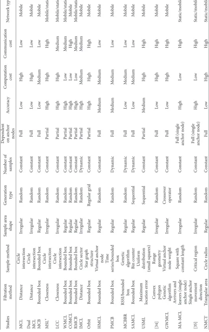
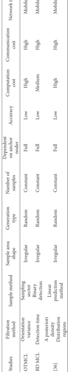
Localization schemes are categorized on the basis of addi-tional hardware requirement, scalability, accuracy, noise, operation environment, and cost, as shown in Table 2. Among all schemes, the range-based one achieves the highest accuracy despite being fully dependent on special hardware. This scheme is followed by the hybrid scheme that utilizes the network connectivity in noise and the RSSI assumption in the normal case. The range-free scheme achieves the lowest accu-racy; location is estimated using network connectivity. SMC locations schemes can be compared in terms of localization accuracy, computational cost, communication cost, a number of samples, dependency on anchor nodes, and network type, as summarized in Table 3.
6.1. Comparison of the Localization Accuracy. Accuracy is a
vital and challenging issue in the localization process. Achiev-ing high accuracy in SMC schemes can be achieved through high anchor nodes density. There are various schemes that fully depend on anchor nodes such as MCL, dual and mixture MCL, MCB, and PMCB, and there are others that combine anchor and normal nodes location information like MSL∗, WMCL, RMCL, COMCL, IMCL, and Orbit. Relying on anchor nodes increases the dependency on the hardware (each anchor node requires a GPS device) which increases the power consumption, cost, and size, whereas using normal nodes can increase the communication and computational cost. Moreover, location information of normal nodes is an estimated location that embedded with the fraction of error.
anchor nodes exist in the neighbors, PMCB uses a time series to forecast location [75]. The bounding of valid sample area in this method is an irregular shape. It is constructed by the intersection between radio range circles of anchor nodes. For this, the distance between each sample and anchor nodes in the first and second hops is utilized to check whether the sample satisfies the anchor nodes constraints. The main drawbacks of this method are that it highly depends on anchor node density and that it uses inefficient and slow filtration methods.
The MSL∗[71] uses the closeness value of the sample to filter out low weight samples. This method can improve the localization accuracy but produces a high communication between the neighbors. Each node broadcasts its samples and samples weight in each time slot to the neighbors in the first and second hops. The communication cost is highly increased in this scheme but, in our previous research named LCC, the communication cost is reduced by selecting the normal nodes that have high intersection elements with the normal nodes in the neighbor.
The MCB scheme uses the intersection area of the bounded box over the anchor nodes to restrict the valid samples area. The shape of the box is regular; thus, it can easily filter out the invalid samples. Nevertheless, this shape contains an invalid area in some corner. WMCL narrows the bounded box by using the negative effect of two-hop anchor and normal nodes location information to optimize the sample area and enhance localization accuracy. Furthermore, RMCB utilizes the positive effect of the two-hop anchor and normal nodes to optimize the sample area and improve the accuracy in WMCL. It should be noted that WMCL uses the normal node location information in the sample and filter steps, whereas MCB utilizes only the anchor node location information in the filter step. The restriction on the sample area is a challenging issue.
IMCL [69] employs the longest circular sector to filter out the invalid samples and a star graph with one root and five leaves is used in Orbit scheme to improve localization accu-racy [92]. The circular sectors method requires additional computation to find the angle and longest sectors, and finding five nodes in the neighbor is inapplicable in each time slot.
The MCL sampling and Laplace’s method use the statisti-cal posterior prediction to filter out invalid samples. However, the improvement of accuracy is minimum and requires high computation [77]. Storing posterior location information of estimated location, velocity, direction, and motion type in the table needs more memory and can slow the localization process in SMCLA [78]. Another localization scheme is genetic algorithm implemented in SMC technique to filter out invalid samples [83]; the genetic algorithm requires large data and high execution time, so it is unsuitable for thin devices like sensor node.
The fast method and precious filtration of invalid samples are essential in mobile WSNs location estimation. Filtration within the irregular shape can be tedious, as it requires repetition of the filtration and sampling steps for several times to generate the valid samples. The bounded box method can constrain the sample area fast and improve the accuracy at the same time. The circular sector and star graph require
high normal node density in the neighbor which may not exist all the time. Statistical and genetic methods require large memory and instruction for execution. Thus, they are incompatible with a thin device like sensor node.
6.2. Comparison of Computation Cost. A fast location
esti-mation is desirable in mobile WSNs location estiesti-mation. A slow sampling method can delay the movement and the sensor may move to other locations before generating enough valid samples. The computational cost is mainly counted by the number of iterations required to generate enough valid samples.
The amount of filtration is a function of both sampling method and shape of the sample area. MCL, Dual and mixture MCL and MSL∗ generate samples randomly over previous samples within the sample area limited by a circle with a radius of maximum velocity. The sample and filter steps are repeated up to 1,000 times in some cases to find valid samples. This weakness is from the irregular shape of the sample area and filtration strategies. The MSL∗ has advantages in keeping the highly weighted sample from the previous time slot. Thus, the new sample is generated over a low weighted sample. Dual and mixture MCL schemes are inverting the probability function in the dual Monte Carlo scheme during the sample and filter steps to improve local-ization accuracy [56]. The disadvantages of these schemes are high computational cost and low sample efficiency.
Bounding of sample area becomes more precise and the sampling efficiency improved by using anchor node bounded box intersection in the MCB scheme, in which the amount of filtration is reduced to 100 times per each sample. WMCL reduces the sample area by 78% and increases the sampling efficiency up to 95%. Moreover, WMCL uses the normal node location information in the sample and filter steps, whereas MCB utilizes only the anchor node location information in the filter step. RMCB improves the sample area and efficiency in WMCL by utilizing a positive anchor node effect behind the negative effect used in WMCL. The anchor node movement directions such as moving backward and moving forward are utilized in COMCL to maintain the sample area over WMCL assumption.
The aforementioned schemes used a static number of samples which is equal to 50 in different sample area size. In PMCB and IMCL schemes, the number of samples is based on the percentage of the sample area with respect to the maximum area of one anchor node in the neighborhood, as represented in (3). However, at least one anchor node is assumed to be in the first hop of the blind node neighbor in most simulations.
Sample number= (50 ∗ (Δ𝑥) ∗ (Δ 𝑦))
4𝑅2 , (3)
whereΔ𝑥andΔ𝑦are the height and length of the bounded box (sample area), respectively, and4𝑅2is the maximum area of one anchor node in the first hop.
[93] divided the sample area into small squares and the sample is distributed uniformly over the squares. The polygon shape property is used to construct the sample area in [34], where the location and number of anchor nodes are used to maintain the polygon shape.
Large number of iterations can slow the location esti-mation and consume more power. The main difficulty in the localization process is the shape of the sample area. Generating valid sample from the irregular shape is a tedious issue. The bounded box method can maintain the shape of the sample area to become a regular shape. Generating sample from such area is an easy thing and can reduce the number of iterations required to generate the valid sample. Dividing the sample area of the small bins or distributing sample uniformly over small squares is weak assumption and is unable to present the reality of the sample area; the using of random generation is more precise and can be more general. Adapting the number of samples with sample area size is an important thing but the most important issue is the efficiency of the sampling method.
6.3. Comparison of Communication Costs. The number of
messages sent is the function of anchor node density in the schemes such as MCL, MCB, and dual MCL; and this number is equivalent to the anchor node number (𝐴) in the neighborhood. In MSL∗and MSL, the normal node location information is utilized along with the anchor node. The normal node in MSL∗ broadcasts the samples in each time slot to the first and second hops, whereas the normal node in MSL only broadcasts its coordinates and not all samples. The communication costs of MSL∗and MSL are represented by
(𝑁 ∗ 𝑆 + 𝐴)and(𝑁 + 𝐴), respectively, where𝑁is the number of normal nodes,𝑆is the number of samples in each time slot (50 samples), and𝐴is the number of anchor nodes in the neighborhood.
Among all schemes, the MSL∗ scheme achieves the highest communication cost, whereas MCL achieves the lowest communication cost. In our LCC scheme, the com-munication cost in MSL∗is reduced by 18% by selecting the closed normal node in the neighborhood.
The assumption in MSL∗ is adopted in WMCL and RMCL; the normal node broadcasts its sample to the first hop. WMCL and RMCL modify the sample with the information on message size; the location of the maximum error is defined in𝑥-axis and𝑦-axis. The COMCL scheme embeds the range of the bounded box from the previous time slot in the sample of the normal node. However, the communication cost of COMCL is 1.04 times higher than that of WMCL. The simulation results in WMCL show that the communication cost is more significantly affected by the size of the message than by the densities of the anchor and normal nodes.
MSL∗ broadcasts the message with information on the IP header, transmitter ID, estimated position, number of hops, and coordinates of 50 valid samples in the previous time unit; this information costs 634 bytes. The normal node messages in WMCL or BB (bounded box) combine the IP header, transmitter ID, estimated position, number of hops, valid samples, and maximum error in𝑥-axis and𝑦-axis; this
information costs only 46 bytes. The normal node message in the IMCL scheme has a size of 66 bytes by combining the IP header, transmitter ID, estimated position, number of hops, valid samples, and eight sectors. The MCL, MCB, and dual MCL schemes yield the lowest communication costs because they only utilize the anchor node location information. The details of bytes sent in each scheme per time slot are listed in [69].
The number of messages is also affected by the number of hops used in the localization process. Normally, SMC utilizes the sensor in the first and second hops. However, the sensor node in the second hop can maximize the communication, especially when normal node samples are used. For example, MSL∗uses the normal node samples of the first and second hops; each anchor node and normal node broadcast their respective samples in each time slot to the first and second hops’ neighbors. Therefore, MSL∗requires a high communi-cation cost.
Table 3 presents the comparison between SMC schemes based on effective parameters. The localization accuracy is the most important variable especially when sensors move in high speed. Most of the schemes improve the localization by utilizing normal nodes location information that highly increases the communication and computation cost.
7. Discussion of Future Works and
Localization Issues
Range-based schemes achieve a higher localization accuracy than range-free schemes. However, range-based schemes are highly dependent on additional hardware that consumes a large amount of power and increases the size and cost of sensor nodes, especially in a dense deployment. The battery replacement of sensor nodes is difficult, particularly when nodes are in remote and hazardous areas. Moreover, commu-nication range and hardware signals are affected by noise and obstacles. Therefore, range-based schemes are unsuitable for certain types of applications.
By contrast, range-free schemes estimate locations using network connectivity and without any additional hardware. A range-free scheme is a challenging area. The obstacle of SMC is its dependency on anchor node density and a high number of valid samples to estimate an accurate location. Repeating the sample and filtering stages several times is a time-consuming process. Furthermore, hop distance schemes require a uniform distribution of anchor nodes, and fingerprint schemes are time-consuming because expert personnel are required to create the offline database and update the database every time the environment changes.