Simulation Algorithm That Conserves Energy and Momentum for Molecular Dynamics of Systems Driven by Switching Potentials

Volume 2009, Article ID 215815,14pages doi:10.1155/2009/215815

Review Article

Simulation Algorithm That Conserves

Energy and Momentum for Molecular Dynamics

of Systems Driven by Switching Potentials

Christopher G. Jesudason

Department of Chemistry, University of Malaya, 50603 Kuala Lumpur, Malaysia

Correspondence should be addressed to Christopher G. Jesudason,[email protected]

Received 26 November 2008; Revised 10 March 2009; Accepted 28 May 2009

Recommended by Jerzy Warminski

Whenever there exists a crossover from one potential to another, computational problems are

introduced in Molecular Dynamics MD simulation. These problem are overcome here by

an algorithm, described in detail. The algorithm is applied to a 2-body particle potential for a hysteresis loop reaction model. Extreme temperature conditions were applied to test for

algorithm effectiveness by monitoring global energy, pressure and temperature discrepancies in

an equilibrium system. No net rate of energy and other flows within experimental error should be observed, in addition to invariance of temperature and pressure along the MD cell for the said system. It is found that all these conditions are met only when the algorithm is applied. It

is concluded that the method can easily be extended to Nonequilibrium MDNEMDsimulations

and to reactive systems with reversible, non-hysteresis loops.

Copyrightq2009 Christopher G. Jesudason. This is an open access article distributed under

the Creative Commons Attribution License, which permits unrestricted use, distribution, and reproduction in any medium, provided the original work is properly cited.

1. Introduction

that forces the system to adopt on average a canonical or microcanonical distribution of energies among the principle components within the system. In synthetic methods, the ”actual” trajectory is not traced, but one that reproduces a canonical trajectory, but even here, opinions differ as to how accurately these trajectories are traced. Indeed, recent work seems to show that external perturbations can modify the ”noise” spectrum of a natural system. For instance, the presence of an external random contribution to a high-frequency periodic electric field can reduce the total noise power12. This suggests that some natural properties connected to time correlation functions is a function of external perturbations and so one may conclude that basic synthetic methods may not include such elements of stochasticity. Another interesting observation of 12,13is the use of Monte Carlo techniques to model the system. In this case, Monte Carlo is used to simulate the dynamics of electrons in the semiconductor lattice by taking into account stochastic averaging. This is to be contrasted with the method here of attempting directand approximateintegration of the equations of motion, moderated by probabilistic inputs of energy at the ends of the box to simulate a ”thermostat.” One guess is that such Monte Carlo methods might be suitable if the details of molecular motion are not being investigated, and that given that a particular form of behavior is accepted, then one might superimpose stochasticity upon it through a Monte Carlo algorithm to simulate scattering phenomena, which includes temperature control. One possible problem with synthetic methods is that if a phenomenon is due to the system being in a particular phase space of a particular fixed Hamiltonian, then such events may not be detected or may be underrepresented in these synthetic methods. An overview of some of the above is in order. In the Nos´e-Hoover method, one defines a Lagrangian for the system coordinates{˙ri,˙pi}as

LNose N

i1

mi 2 s

2_˙r2 i − U

rNQ 2s˙

2₋L

β lns, 1.1

where β is the temperature parameter. This so-called Lagrangian defines the conjugate momenta to ri ands as, respectively, pi mis2˙ri and ps Qs˙. Then for this system, there results ultimately a pseudo-Hamiltonian:

HNose N

i1

mi 2 s

2_p2 i − U

rNQ 2ξ

2L

βlns, 1.2

whose trajectory is determined by the coupled equations that must be solved:

˙ri pi

mi

,

˙pi

∂Uri ∂˙ri −

ξpi,

˙

ξ

ipi2/m−L/β

Q ,

˙

s

s

dlns

dt ξ,

where the last equation in superfluous. Equation 1.3 is solved by special and time consuming techniques that are not typical of those used for the standard Hamiltonian, such as the well-known Verlet and Gear algorithms. An analogous set of equations can be derived for constant pressure studies14. Another algorithm to correct for machine errors in following a PES is temperature-coupling method of Berendsen et al.15which has been widely used in many systems but it is claimed11, page 161that the canonical distribution is not produced ”exactly.” In this method, the velocities are scaled every time step by factorλgiven by

λ

1 δt

τT

T0

T −1

1/2

. 1.4

The upshot of the above is that these algorithms can be viewed as some sort of corrective procedure used to overcome problems of trajectory calculation accuracy for the rather simplistic, single-valued potential that are used for nonreactive systems due to the nonperfect integration of the equations of motion 16. Paradoxically perhaps, the theories that were developed never allude to the machine error basis behind equilibrium thermostatting, which is not required by theHtheorem when the system relaxes to equilibrium, and thus hardly any reference is made to the error in the computations of their new equations of motion that incorporates fixed thermodynamical variables like the pressure or temperature. It may be argued that they were referring to the canonical ensemble, but a careful examination of the Nos´e justification of the method refers to a microcanonical phase space trajectory with the delta function having a component form δH− E α. This might imply that machine error was not the foremost reason for the invention of the algorithms together with the accompanying theory. To date however, there has been little—if any—development in providing corrective measures to trajectory calculations for multivalued and other potentials which require switches to transfer trajectories from one PES to another for various molecular species which involve the variables pertaining to the surfaces. This particular review refers to one such attempt, which will be described in detail in what follows.

−10

−5

0 5 10 15 20

Potential

ener

gy/LJ

unites

0.8 1 1.2 1.4 1.6 1.8

r/LJ distance units

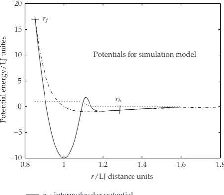
Potentials for simulation model

uLJintermolecular potential

srswitiching function Atomic LJ potential

rf

rb

Figure 1: Potentials used for this work.

The model reaction simulated may be written as

2Ak1

k−1

A2, 1.5

where k1 and k−1 are the forward and backward rate constant, respectively. The reaction simulation was conducted at high temperatures not used ordinarily in simulations of LJ Lennard-Jones fluids where the reduced temperatures T∗ all units used are reduced LJ ones 17 ranges ∼0.3–1.2,17 whereas here, T∗ ∼ 8.0–16.0, well above the supercritical regime of the LJ fluid. At these temperatures, the normal choices for time step increments do not obtain without also taking into account energy-momentum conservation algorithms in regions where there are abrupt changes of gradient11,17,18. The global literature does not seem to cover such extreme conditions of simulation with these precautions. The simulation was at densityρ0.70 with 4096 atomic particles. The potentials used are as given inFigure 1 whererb 1.20 for the vicinity where the bond of the dimer is broken2 free particles emerge andrf 0.85 is the point along the hysteresis potential curve where the dimer is defined to exist for two previously free particles. The reaction proceeds as follows: all particles interact with the splined LJ pair potentialuLJexcept for the dimeric pairi, jformed from particlesi andjwhich interact with a harmonic-like intermolecular potential modified by a switchur

given by

ur uvibrsr uLJ1−sr, 1.6

whereuvibris the vibrational potential given by1.7

uvibr u0 1

2kr−r0

The switching functionsris defined as

sr 1

1 r/rswn, 1.8

where

sr−→1 ifr < rsw,

sr−→0 for r > rsw.

1.9

The switching function becomes effective when the distance between the atoms approach the value rsw see Figure 1. Some of the other parameters used in the equations that follow include u0 −10, r0 1.0, k ∼ 2446 exact value is determined by the other input parameters,n 100, rf 0.85, rb 1.20, andrsw 1.11. Switches are commonly encountered in theoretical accounts of complex interactions, such as found in polymer interactions and in chemical reactions. There are many flavors of switch categories, and some are more effective than others in forcing the merging of one potential type to another for a given distance defined by a metric19–23. The ideal switch would resemble a Heaviside step function but such functions cannot be so easily incorporated into the dynamical equations of motion which feature continuous variables because the various orders of differentials must be defined and computable over the discrete time steps. For instance, a switching function with several known applications, including those from statistical mechanics is given by the form19:

SR 1−tanhaR−Reb

, 1.10

whereaandbare defined constants and theRs represent distances. For various optimization schemes to check for global minima, such as claimed in the Hunjan-Ramaswamy global optimization method, switches such as thegtfunction of the following form has been used 20:

gt exp−ζtcos2_{3πζt1−λζt, 1.11}

wheretis a time-dependent variable. On the other hand, for cluster dynamics, a switch of the form21, equation 7,

Φr tanh r−E

F

, 1.12

switching functions SW to demarcate potential boundaries23, equations 5, 6about bonding anglesθand bond distancesrhaving the forms below have been used:

SWθabc 1−cos16θabc

4

,

SWrab 1−tanharab−Rerabb8

.

1.13

The temperature T and pressure p are computed by the equipartition and Virial expression given, respectively, by

N

i1pi·pi

mi

3NkBT, P ρkBT

W

V , 1.14

whereW −1/3_{i j>i}wrijand the intermolecular pair Virialwris given bywr rdvr/drwithvbeing the potential.

2. Algorithm and Analysis of Numerical Results

The velocity Verlet algorithm 25, page 81 used here 17 and allied types generate a trajectory at timenδtfrom that atn−1δtwith step incrementδtthrough a mappingTm, wherevnδt, rnδt Tmvn−1δt, rn−1δtwhich does not scale linearly withδt. This follows from the form used here consisting of 3 steps in computing the trajectory at time

tδtfrom the data at timet:

v t1

2δt

vt 1

2δtat,

rtδt rt δtv t1

2δt

,

vtδt v t1

2δt

1

2δtatδt.

2.1

For a Hamiltonian H whose potential V is dependent only on position r having momentum components pi, the system without external perturbation has constant energy

E, and the normal assumption in MDNEMDis that for thenth step,ΔEn|Hnδt−E| ≤ and alsoN_i1ΔEi≤sfor the specifieds. In the simulation under NEMD, the force fields are constant and do not change for any one time step. In these cases, the energy is a constant of the motion for any time intervalδtT when no external perturbationse.g., due to thermostat interference are impressed. When there is a crossing of potentials at such a time interval fromφb to φa at an interparticle distance icdrc such as pointsrf and rb ofFigure 1 of general particle 1 and 2 the1,2 particle pairdue to a reactive processsuch as occurs in either direction of1.5, a bifurcation occurs where the MD program computes the next step coordinates as for the unreacted systempotentialφb, which needs to be corrected. Let the icd at time stepiberi withφb potentialand at stepi1 after intervalδtberf ri1 whererf < rc < ri. Due to this crossover, a different HamiltonianHis operative after point

Theorem 2.1. A virtual potential which scales velocities to preserve momentum and energy can be

constructed about regionrc.

Proof. The external work done δW on particles 1 and 2 over the time step is proportional

to the distance traveled since these forces are constant and so for each of these particlesi, Fext,i ·Δri δWi where Δri is the distance increment during at least part of the time step

fromrctorf. For the nonreacting trajectory over timeλδtλ≤1 virtual because it is not the correct path due to the crossover atrc,

δW2δW1−

φb

rf

−φbrc ΔK.E., 2.2

whereΔK.E.is the change of kinetic energy for the1,2pair from the First Law between the end pointsrf, rc. Now over time intervaltctotf, for the reactive trajectory, we introduce a ”virtual potential”Vvir_{that will lead to the same positional coordinates for the pair at the} end of the time step with different velocities than for the nonreactive transition leading to the transition

δW2δW1−

Vvirrf

−Vvirrc Δ

K.E., 2.3

whereΔK.E.is the change of kinetic energy for the pair withVvir_{turned on and along} this trajectory, the change of potential forVvir_{is equated to the change in the K.E. of the pair} as given in the results ofTheorem 2.2for all three orthogonal coordinates, that is,

δVvirr−δφbr δ

ΔK.E.x,y,z

−Δ K.E._x,y,z

, 2.4

with momentum conservation, that is, δVvir_{ri δφari for the variation along the r} i coordinate, but δφari −δK.E.along internuclear coordinate ri whereas δVvir −K.E. scaled about all three axes. Continuity of potential implies

φa

rf

Vvirrf

; φarc Vvirrc; φbrc Vvirrc. 2.5

Subtracting2.2from2.3and applying b.c.’s2.5leads to

Δ φb

rf

−Vvirrf

φb

rf

−φa

rf

Eb−Ea

Δ K.E.−ΔK.E..

2.6

The above shows that a conservative virtual potential could be said to be operating in the vicinity of the transitionfromtc tota.

Theorem 2.2. Relative to the velocities at anyrf due to theφbpotential, the rescaled velocities vdue

to the potential differenceΔleading to these final velocities due to the virtual potential can have a form

given by

v

i 1αviβ, 2.7

(wherei1,2) for a vectorβ.

Proof. From the v velocities atrfdue toφb, we compute the vvelocities atrfdue to the virtual

potential. Since net change of momentum is due to the external forces only, which is invariant for the1,2pair, conservation of total momentum relating vand v in2.7yields a definition ofβsummation from 1 to 2 for what follows, where the mass of particleiismi

β−α

mivi

mi

. 2.8

Defining for any vector s, s2_s.s,β2 _α2_{Q, where}

Q

mivi2

mi2 , 2.9

then the rescaled velocities become from2.7

v

i2 1α2vi221αvi·ββ2. 2.10

WithΔ Eb−Ea, energy conservation implies

1 2miv

i2−

1 2mivi

2 _{Δ. 2.11}

The coupling of2.10and2.11leads, after several steps of algebra to

Δ α2m1m2 2m1m2

v12v22−2v1·v2

2αm1m2 2m1m2

v12v22−2v1·v2

.

2.12

Defininga v1−v22,qm2m1/2m1m2,q >0, a≥0, then the above is equivalent to the quadratic equation:

α2qa2qaα−Δ 0, 2.13

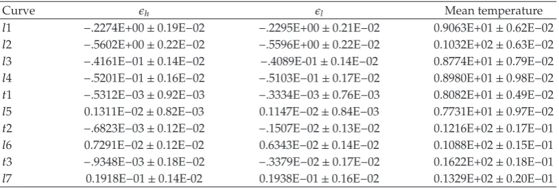
Table 1: Values for the mean heat supply per unit step and temperature. The error is one unit of standard error for the quantities.

Curve h l Mean temperature

l1 −.2274E00±0.19E−02 −.2295E00±0.21E−02 0.9063E01±0.62E−02

l2 −.5602E00±0.22E−02 −.5596E00±0.22E−02 0.1032E02±0.63E−02

l3 −.4161E−01±0.14E−02 −.4089E-01±0.14E−02 0.8774E01±0.79E−02

l4 −.5201E−01±0.16E−02 −.5103E−01±0.17E−02 0.8980E01±0.98E−02

t1 −.5312E−03±0.92E−03 −.3334E−03±0.76E−03 0.8082E01±0.49E−02

l5 0.1311E−02±0.82E−03 0.1147E−02±0.84E−03 0.7731E01±0.97E−02

t2 −.6823E−03±0.12E−02 −.1507E−02±0.13E−02 0.1216E02±0.17E−01

l6 0.7291E−02±0.12E−02 0.6343E−02±0.14E−02 0.1088E02±0.15E−01

t3 −.9348E−03±0.18E−02 −.3379E−02±0.17E−02 0.1622E02±0.18E−01

l7 0.1918E−01±0.14E-02 0.1938E−01±0.16E−02 0.1329E02±0.20E−01

The above Inequality leads to a certain asymmetry concerning forward and backward reactions, even for reversible reactions where the regions of formation and breakdown of molecules are located in the same region with the reversal of the sign of approximateΔ. For this simulation, a reaction in either directionformation or breakdown of dimer proceeds if2.12is true for realα; if not, then the trajectory follows the one for the initial trajectory without any reaction i.e., no potential crossover. We would like to suggest that the real reasons for shifted potentials showing ”instability in the numerical solution of the differential equations”25, page 146, line 5has nothing to do with the forces being discontinuous. It will be recalled that this potential vS _{has the form v}S_r

ij vrij−vc for 0 < rij ≤ rc, andvS _{0 otherwise withv}

c vrc. This is because the potentials are continuous and by Newton’s Third Law there can be no net change in the momentum due to intermolecular forces implying momentum conservation. Further, the energiesboth kinetic and that for the continuous potentialcannot change over an instantaneous change of the forces over zero distance. Thus there is also energy conservation. The reason for the instabilities is due to the fact that the change of position is calculated from the forces of the previous step before the sudden change in force, that puts the particle position away from the PES where there is no mechanical algorithm to correct for the violation in energy conservation with respect to the PES and the kinetic energy. Hence, the problem has nothing to do with the mechanical or dynamical setup of the potential and the forces, but with the MD move algorithm that cannot handle effectively discontinuities of the forces.

Interpretation of Results

Figure 1shows a rapidly changing potential curve with several inflexion points used in the simulation at very high temperatureas far as I know such ranges have not been reported in the literature for nonsynthetic methodswarranting smaller time steps; larger ones would introduce errors due to the rapidly changing potential and high K.E.; thus, even with the application of the algorithm about coordinates rf and rb, curves l1 andl2 have too large

δtvalue to achieve equilibrium—meaning flat or invariant—temperature seeFigure 2 or pressureseeFigure 3or unit step thermostat heat supplyseeTable 1.handlprofiles where for these curves, theh, lvalues show net heat absorption.

6 8 10 12 14 16 18

T

emperatur

e/LJ

units

0 20 40 60 80

xlayer number

l1

l2

l3

l4

t1

l5

t2

l6

t3

l7

Figure 2: Temperature profile across the cell for different set conditionsa−efor temperatureT∗and step

timeδtpairsT∗, δtwherea 8.0,2.0ep−3, b 8.0,5.0ep−4, c 8.0,5.0ep−5, d 12.0,5.0ep−

5, e 16.0,5.0ep−5. The curves{l1, l3, t1, t2, t3}results with the application of the algorithm atrband

rf with associated conditionsl1⇔a, l3⇔b, t1⇔c, t2⇔d, t3⇔ewhile the curves{l2, l4, l5, l6, l7}are

for the cases without implementing the algorithm with the associated conditionsl2⇔a,l4⇔b,l5⇔c,

l6⇔d,l7⇔e, whereep x≡10x_.

14 16 18 20 22 24 26 28

Pr

essur

e/LJ

u

nits

0 20 40 60 80

xlayer number

l1

l2

l3

l4

t1

l5

t2

t6

l3

l7

Figure 3: Pressure profile across the cell for different runs. The conditions of the runs and the labeling of

this choice of time step interval was found adequate for runs at much higher temperatures T 12 andT 16which was used to determine thermodynamical properties18. For this

δtvalue and all others, no reasonable stationary equilibrium conditions could be obtained without the application of the algorithmcurvesl2,l4,l5,l6 andl7. The algorithm is seen to be effective over a wide temperature range for this complex dimer reaction simulated under extreme values of thermodynamical variables and the results here do not vary for longer runs and greater sampling statistics e.g., 6 or 10 million time steps. The thin, pencil-like geometry of the rectangular cell with thermostats located at the ends would highlight the energy nonconservation leading to a nonflat temperature distribution, as observed and which was used to determine the regime of validity of the algorithm.

3. Conclusions

Without difficulty, one can easily construct a reversible system where rf and rb coincide, and this will be investigated next. Such systems would typically have most of the particles in the molecular or dimer state, and accumulated machine computational errors would be one factor to consider which this algorithm should effectively address. The two body potentials considered here saves time but the methodology is general and applies to all

n-body interactions, because the essential kinetics and dynamics of all physical phenomena are governed by the principle of conservation of energy and momentum without exception. This element has often been bypassed or has received little emphasis in non-Hamiltonian and other synthetic methodologies used currently.

Acknowledgment

The author is grateful to University of Malaya for a Conference grant to present this algorithm as an Invited Speaker at the Fifth ICDSA2007, Atlantawhich this communication briefly reviews.

References

1 http://www.charmm.org.

2 http://www.gromacs.org.

3 http://www.cse.scitech.ac.uk/ccg/software/DL POLY.

4 http://www.itap.physik.uni-stuttgart.de/imd.

5 http://ambermd.org.

6 J. Xu, S. Kjelstrup, and D. Bedeaux, “Molecular dynamics simulations of a chemical reaction;

conditions for local equilibrium in a temperature gradient,” Physical Chemistry Chemical Physics, vol. 8, pp. 2017–2027, 2006.

7 S. Nos´e, “A unified formulation of the constant temperature molecular dynamics methods,” The

Journal of Chemical Physics, vol. 81, no. 1, pp. 511–519, 1984.

8 S. Nos´e, “A molecular dynamics method for simulation in the canonical ensemble,” Molecular Physics,

vol. 52, pp. 255–268, 1984.

9 W. G. Hoover, “Canonical dynamics: equilibrium phase-space distributions,” Physical Review A, vol.

31, no. 3, pp. 1695–1697, 1985.

10 W. G. Hoover, “Constant-pressure equations of motion,” Physical Review A, vol. 34, no. 3, pp. 2499–

2500, 1986.

11 D. Frenkel and B. Smit, Understanding Molecular Simulations: From Algorithms to Applications, vol. 1 of

Computational Science Series, Academic Press, San Diego, Calif, USA, 2nd edition, 2002.

12 D. Persano Adorno, N. Pizzolato, and B. Spagnolo, “The influence of noise on electron dynamics

in semiconductors driven by a periodic electric field,” Journal of Statistical Mechanics: Theory and

13 D. Persano Adorno, M. Zarcone, and G. Ferrante, “Far-infrared harmonic generation in semiconduc-tors: a Monte Carlo simulation,” Laser Physics, vol. 10, no. 1, pp. 310–315, 2000.

14 G. J. Martyna, D. J. Tobias, and M. L. Klein, “Constant pressure molecular dynamics algorithms,” The

Journal of Chemical Physics, vol. 101, no. 5, pp. 4177–4189, 1994.

15 H. J. C. Berendsen, J. P. M. Postma, W. F. Van Gunsteren, A. DiNola, and J. R. Haak, “Molecular

dynamics with coupling to an external bath,” The Journal of Chemical Physics, vol. 81, no. 8, pp. 3684– 3690, 1984.

16 M. E. Tuckerman and G. J. Martyna, “Understanding modern molecular dynamics: techniques and

applications,” Journal of Physical Chemistry B, vol. 104, no. 2, pp. 159–178, 2000.

17 J. M. Haile, Molecular Dynamics Simulation, John Wiley & Sons, New York, NY, USA, 1992.

18 C. G. Jesudason, “Model hysteresis dimer molecule. I. Equilibrium properties,” Journal of Mathematical

Chemistry, vol. 42, no. 4, pp. 859–891, 2007.

19 T. Baer and W. L. Hase, Unimolecular Reaction Dynamics, Oxford University Press, Oxford, UK, 1996.

20 Z. G. Fthenakis, “Applicability of the Hunjan-Ramaswamy global optimization method,” Physical

Review E, vol. 70, no. 6, Article ID 066704, 8 pages, 2004.

21 G. S. Fanourgakis and S. C. Farantos, “Potential functions and static and dynamic properties of

Mgm_Ar

nm1,2;n1−18clusters,” Journal of Physical Chemistry, vol. 100, pp. 3900–3909, 1996.

22 D. R. Bevan, L. Li, L. G. Pedersen, and T. A. Darden, “Molecular dynamics simulations of the

dCCAACGTTGG2decamer: influence of the crystal environment,” Biophysical Journal, vol. 78, no.

2, pp. 668–682, 2000.

23 E. Duffour and P. Malfreyt, “MD simulations of the collision between a copper ion and a polyethylene

surface: an application to the plasma-insulating material interaction,” Polymer, vol. 45, no. 13, pp. 4565–4575, 2004.

24 I. Bena, C. Van den Broeck, R. Kawai, and K. Lindenberg, “Nonlinear response with dichotomous

noise,” Physical Review E, vol. 66, no. 4, Article ID 045603, 4 pages, 2002.

25 M. P. Allen and D. J. Tildesley, Computer Simulation of Liquids, Oxford University Press, Oxford, UK,

Submit your manuscripts at

http://www.hindawi.com

Hindawi Publishing Corporation

http://www.hindawi.com Volume 2014

Mathematics

Hindawi Publishing Corporation

http://www.hindawi.com Volume 2014

Mathematical Problems in Engineering

Hindawi Publishing Corporation http://www.hindawi.com

Differential Equations

International Journal of

Volume 2014

Hindawi Publishing Corporation

http://www.hindawi.com Volume 2014 Hindawi Publishing Corporationhttp://www.hindawi.com Volume 2014

Hindawi Publishing Corporation

http://www.hindawi.com Volume 2014

Mathematical PhysicsAdvances in

Complex Analysis

http://www.hindawi.com Volume 2014

Optimization

Hindawi Publishing Corporation

http://www.hindawi.com Volume 2014

Combinatorics

Hindawi Publishing Corporation

http://www.hindawi.com Volume 2014

International Journal of

Hindawi Publishing Corporation

http://www.hindawi.com Volume 2014

Journal of

Hindawi Publishing Corporation

http://www.hindawi.com Volume 2014

Function Spaces

Abstract and Applied Analysis

Hindawi Publishing Corporation

http://www.hindawi.com Volume 2014

International Journal of Mathematics and Mathematical Sciences

Hindawi Publishing Corporation http://www.hindawi.com Volume 2014

The Scientific

World Journal

Hindawi Publishing Corporation

http://www.hindawi.com Volume 2014

Hindawi Publishing Corporation

http://www.hindawi.com Volume 2014

Discrete Dynamics in Nature and Society

Hindawi Publishing Corporation

http://www.hindawi.com Volume 2014

Hindawi Publishing Corporation

http://www.hindawi.com Volume 2014

Discrete Mathematics

Hindawi Publishing Corporation