Constrained nonparametric estimation of
input distance function
Sun, K
http://dx.doi.org/10.1007/s1112301303729
Title
Constrained nonparametric estimation of input distance function
Authors
Sun, K
Type
Article
URL
This version is available at: http://usir.salford.ac.uk/34561/
Published Date
2015
USIR is a digital collection of the research output of the University of Salford. Where copyright
permits, full text material held in the repository is made freely available online and can be read,
downloaded and copied for noncommercial private study or research purposes. Please check the
manuscript for any further copyright restrictions.
(will be inserted by the editor)
Constrained Nonparametric Estimation of Input Distance Function
Kai Sun
the date of receipt and acceptance should be inserted later
Abstract This paper proposes a constrained nonparametric method of estimating an input distance function. A regres-sion function is estimated via kernel methods without functional form assumptions. To guarantee that the estimated input distance function satisfies its properties, monotonicity constraints are imposed on the regression surface via the constraint weighted bootstrapping method borrowed from statistics literature. The first, second, and cross partial analytical deriva-tives of the estimated input distance function are derived, and thus the elasticities measuring input substitutability can be computed from them. The method is then applied to a cross-section of 3,249 Norwegian timber producers.
Keywords Nonparametric estimation·Input distance function·Constraints·Elasticities
JEL CodesC14·D24
Kai Sun
Economics and Strategy Group, Aston Business School, Aston University, Aston Triangle, Birmingham B4 7ET, UK E-mail: [email protected]
1 Introduction
One of the main objectives of productivity analysis is to estimate a representation of technology using econometrics or
data envelopement analysis (DEA), among others. It is well-known that DEA assumes no functional form of a frontier, and
linear programming allows one to impose linear constraints on each observation. However, when it comes to econometric
methods, a functional form is usually required, and information (e.g., marginal cost/product) can be calculated after
parameters are estimated. Researchers should then check if the estimated information follows theoretical properties of
the technology. While using a large micro-level data set, however, it may well be the case that such properties are
not satisfied for a subset of observations. In order to address this issue, Terrell (1996), Rambaldi and Doran (1997),
Ryan and Wales (2000), and Henningsen and Henning (2009), among others, proposed methods of imposing various
constraints on parametric functions. However, it is still a problem to impose these constraints on a nonparametric
function.
In this paper, we provide solutions to the two above-mentioned problems of econometric methods, i.e., functional
forms that are not flexible and theoretical constraints that are difficult to impose. To address the first problem, we
propose estimating a technology without a parametric functional form via nonparametric kernel econometric methods.
Thus, the functional form assumption is relaxed and the technology is estimated in a fully flexible manner. The price
one has to pay for such flexibility, however, is many observations may violate properties of the technology. Therefore, it
is desirable that constraints are imposed on the nonparametric regression function such that the properties are satisfied
for each individual observation. To do this, we apply the new approach of constraint weighted bootstrapping (CWB) first
introduced by Hall and Huang (2001) and further studied by Du et al (2013) and Parmeter et al (2013).
To explore the kernel and the CWB methods, we first need to specify a technology as our main focus. In this paper,
we choose an input distance function (IDF) because although the functional form of an IDF is generally unknown
(F¨are et al, 1994), many past and more recent studies have sought to estimate parametric distance functions specifying a
translog functional form and using ordinary least squares (OLS) to estimate the unknown parameters (Lovell et al, 1994;
Grosskopf et al, 1997; Ray, 2003; Cuesta et al, 2009, among others). F¨are et al (1985, 1994) and Coelli and Perelman
(1999), among others, used DEA to estimate the distance function without specifying any functional form. This paper
fills the gap by estimating the IDF using nonparametric econometric methods without any functional form assumption.1
Furthermore, monotonicity constraints based on the properties of the IDF are imposed via CWB.2 Our methodology
extends to other representations of technology in a straightforward manner. As a by-product of the econometric estimation,
the first and second order analytical derivatives of the nonparametric IDF are derived, and thus the elasticities measuring
input substitutability/complementarity can be calculated from them.
As an empirical example, we apply the proposed methodology to a Norwegian forestry data set from Lien et al (2007)
compiled by Statistics Norway. Both the unconstrained and constrained nonparametric IDFs as well as the implied
1 Another primal representation of technology is a production function. A nonparametric production function via kernel regression has
been studied by Henderson (2009), Du et al (2013), among others. Furthermore, the estimation of the production function may require fewer regularities as it is arguable that the marginal product of labor can be negative because of labor hoarding or regulation (Heshmati et al, 2013).
2 An IDF is dual to a cost function, and therefore, it must satisfy conditions similar to those of the cost function. However, estimation
elasticities are estimated and results are compared. We find that without imposing constraints, 18.25% observations violate
one of the theoretical properties of the IDF. The Kolmogorov-Smirnov test shows that the gradients and the elasticities
calculated from the constrained IDF significantly differs from those calculated from the unconstrained counterpart. Finally,
we reported density plots of the estimated Antonelli, Morishima, and Symmetric elasticities of complementarity.
The rest of the paper is organized as follows. Section 2 describes the methodology of the constrained nonparametric
econometric estimation methodology. Section 3 applies the methodology to a real data set. Section 4 discusses limitations
and possible extensions of the current method, and section 5 concludes the paper.
2 Methodology
2.1 Nonparametric Estimation of a Distance Function via Kernel Methods
The distance function representation of a production technology, proposed by Shephard (1953, 1970) does not require
any aggregation, prices, or behaviorial assumptions. Following F¨are and Primont (1995), we first define the production
technology of the firm using the input set,L(Y), which represents the set of allK inputs,X ∈RK+, which can produce
the vector ofQoutputs,Y ∈RQ+. That is:
L(Y) ={X ∈RK+ :Xcan produceY}. (1)
We assume that the technology satisfies the standard axiom of strong disposability. The IDF is then defined on the input
set,L(Y), as:
D(X, Y) = max{ρ: (X/ρ)∈L(Y)}, (2)
whereρ is the scalar distance by which the input vector can be deflated.D(X, Y) satisfies the following properties: (1)
it is non-increasing in each output level; (2) it is non-decreasing in each input level; (3) it is homogeneous of degree 1 in
X.3 It is based on an input-saving approach and gives the maximum amount by which an input vector can be radially
contracted while still being able to produce the same output vector. The IDF,D(X, Y), will take a value which is greater
than or equal to one if the input vector,X, is an element of the feasible input set,L(Y). That is,D(X, Y)≥1 ifX∈L(Y).
The distance function will take a value of unity ifX is located on the inner boundary of the input set.
To empirically estimate the distance function, we first define:
D≡A·D(X, Y), (3)
whereAis the productivity parameter, andX andY are the input and output vectors, respectively. Using property (3)
of the IDF, viz., homogenous of degree 1 inX, we can write (3) as:
D/X1=A·D( ˜X, Y), (4)
3 An input distance function is concave in inputs if the input requirement set,L(Y), is convex (Kumbhakar and Lovell 2000, p.30).
whereX1 is the numeraire input, and ˜X is a vector of input ratios, with elements ˜Xk =Xk/X1, ∀k = 2, . . . , K. Taking
the natural logarithm for both sides gives:
lnD−lnX1= lnA+ lnD( ˜X, Y). (5)
LettingD= 1 would give:4
−lnX1= lnD( ˜X, Y) + lnA
= lnD(exp(ln ˜X),exp(lnY)) + lnA
≡m(ln ˜X,lnY) +v,
(6)
where v = lnA is the noise term, interpreted as the natural logarithm of the productivity parameter.5 Using general
notation, (6) can be written as:
Y=m(z) +v, (7)
whereY=−lnX1,m(·) is the unknown smooth distance function,zis the vector of continuous variables (i.e., ln ˜Xk,∀k=
2, . . . , K; lnYq,∀q= 1, . . . , Q), andvis the random error uncorrelated with any element ofz.
To estimate the unknown function, one can use the local-constant least-squares estimator ofm(z) (see Li and Racine
(2006) for more details), given by:
ˆ
m(z) =
∑n i=1K(
zi−z h )Yi
∑n i=1K(
zi−z h )
, (8)
whereK(·) is a (scalar) Gaussian product kernel weighting function for the continuous variables (see Appendix B for an
explicit expression);ndenotes the sample size;his a vector of bandwidth, with each element for a particular variable in
thez vector.
Estimation of the bandwidths, h, is typically the most salient factor when performing nonparametric estimation.
Although many selection methods exist, we utilize the data-driven least-squares cross validation (LSCV) method.
Specif-ically, the bandwidths are chosen to minimize
n−1
n
∑
i=1
[Yi−mˆ−i(zi)]2, (9)
where ˆm−i(·) = ∑n
j̸=iK( zj−zi
h )Yj ∑n
j̸=iK( zj−zi
h )
is the leave-one-out local-constant kernel estimator ofm(·). We use thenpregbwfunction
from the np package (Hayfield and Racine, 2008) in R (R Development Core Team, 2011) to estimate the bandwidth
vector. This bandwidth vector is then plugged into (8) to estimate the IDF.
To calculate the derivatives of the distance function with respect to each input and output, (6) can be re-written as:
lnD= lnX1+m(ln ˜X2, . . . ,ln ˜XK,lnY1, . . . ,lnYQ) +v. (10)
4 Alternatively, the estimating equation can be derived by definingD(X, Y)≡1/A, and then imposing the homogeneity restriction and taking the natural logarithm. We would like to thank an anonymous referee for the suggestion.
For example, the first partial derivatives of interest, that should be investigated to guarantee the monotonicity properties
of the IDF, are:
∂lnD ∂lnX1
= 1− K
∑
k=2
∂m ∂ln ˜Xk
, (11)
∂lnD ∂lnXk
= ∂lnD
∂ln ˜Xk
= ∂m
∂ln ˜Xk
, ∀k= 2, . . . , K,6 (12)
and
∂lnD ∂lnYq
= ∂m
∂lnYq
, ∀q= 1, . . . , Q, (13)
where the first partial derivative ofm(·) with respect to a particular argument, say,zl∈ {ln ˜X2, . . . ,ln ˜XK,lnY1, . . . ,lnYQ},
is ∂m ∂zl = n ∑ i=1 (
zli−zl h2
l
)
K(·)∑iK(·)−K(·)∑i
[(
zli−zl h2
l
) K(·)
]
(∑iK(·))2 ·(−lnX1i). (14)
See Appendix B for detailed derivation of the first and the second partial derivatives ofm(·) with respect tozl, and the
cross partial derivatives with respect tozlandzk,∀l̸=k.
2.2 Imposition of Regularity Constraints
Recall that the IDF has the following theoretical properties:
∂lnD ∂lnXk ≥
0, ∀k= 1, . . . , K (15)
and
∂lnD ∂lnYq ≤
0, ∀q= 1, . . . , Q.7 (16)
However, when it comes to empirical estimation, it is very likely for one to obtain violations of these properties for some
individual observation. Most empirical researchers check these regularity conditions at the mean of the data instead of
every data point, and report results evaluated at the mean. This practice defeats the purpose of using micro data. Results
may not be of much use for policy analysis if the theoretical restrictions are violated for many individual producers. Instead
of ignoring results that violate rationality, we use a new statistical method that imposes these economic constraints. We
then calculate the gradients of the IDF and the elasticities based on that all these joint constraints are satisfied.
In order to impose such observation-specific inequality constraints, we follow the constraint weighted bootstrapping
(CWB) method first proposed by Hall and Huang (2001) and further studied by Du et al (2013) and Parmeter et al
(2013), whose idea is to transform the response variable by assigning observation-specific weights such that certain
constraints in the model are satisfied. To illustrate this methodology, let{Yi, zi}ni=1 denote sample pairs of response and
explanatory variables, whereYiis a scalar,8 zi is of dimension (K+Q−1), andndenotes the sample size. The goal is to
estimate the conditional mean modelY=m(z) +v, subject to constraints on the first order gradient of the l-th element
6 By chain-rule,∂lnD/∂lnX
k=∂lnD/∂ln ˜Xk,∀k= 2, . . . , K.
7 SinceD,X
k, andYqare all non-negative, ∂∂lnlnXD
k ≥0 implies
∂D
∂Xk ≥0, and
∂lnD
∂lnYq ≤0 implies
∂D ∂Yq ≤0. 8 Y
inz,ml(z) =∂m(z)/∂zl, wherezl is thel-th element of the vectorz, or on a linear combination of any of the first order
gradients.
We can express the local-constant estimator as:
ˆ
m(z) =n·
n
∑
i=1
Ai(z)n−1Yi, (17)
where Ai(z) = K(zi
−z h ) ∑n
i=1K(zi
−z h )
, K(·) and hare defined the same as in (8).9 The first order gradient of the local-constant
estimator, ˆml(z), can be expressed as:
ˆ
ml(z) =n· n
∑
i=1
Ai,l(z)n−1Yi, (18)
whereAi,l(z) =∂Ai(z)
∂zl (see Appendix B for an explicit expression of the derivative ofAi(z) with respect tozl). Therefore,
a particular linear combination of these first order gradients is:
1− K∑−1
l=1 ˆ
ml(z) = 1− K∑−1
l=1 ( n· n ∑ i=1
Ai,l(z)n−1Yi
)
, (19)
which is used to impose constraints in the form of (11).
To impose the monotonicity constraints, re-write (18) and (19) as:
ˆ
ml(z|p) =n·
n
∑
i=1
Ai,l(z)piYi, ∀l= 1, . . . , K+Q−1, and (20)
1− K∑−1
l=1 ˆ
ml(z|p) = 1− K∑−1
l=1 ( n· n ∑ i=1
Ai,l(z)piYi
)
, (21)
wherepi is the weight for the ith observation of the responseY, and
∑n
i=1pi = 1.10 Ifpi= 1/n (i.e., uniform weights),
then the constrained estimator will reduce to the unconstrained estimator.
The goal is to transform the response as little as possible through the weights such that the constraints are satisfied.
The following is the weight selection criterion proposed by Du et al (2013) and Parmeter et al (2013):
p∗= argminD(p) = (pu−p)′(pu−p)
st.l(z)≤mˆl(z|p)≤u(z), ∀l= 1, . . . , K+Q−1, and
l(z)≤1− K∑−1
l=1 ˆ
ml(z|p)≤u(z),
(22)
9 The CWB method is also applicable to the local-linear kernel estimator. This is because (17) becomes the local-linear estimator
(Li and Racine, 2004) if we write
Ai(z) =
{∑n
i=1 K
( zi−z
h ) [
1 zi−z
zi−z(zi−z)(zi−z)′
]}−1 K
( zi−z
h ) [
1 zi−z
]
Note that theAi(z) in the local-linear case is a 2×1 block vector. The first element of it is the conditional mean, and the second element
gives the gradient vector.
10 Du et al (2013) showed that p
i can be either positive or negative for the purpose of imposing generalized constraints. In contrast,
wherep∗is a vector of optimal weight for each response observation,D(p) is anL2metric,puis a vector of uniform weights
(i.e., 1/n), which can also be viewed as an initial search condition,l(z) andu(z) represent observation-specific lower and upper bounds for ˆml(z | p), respectively. If l(z) = 0 and u(z) = +∞, then we can impose monotonically increasing constraints; if u(z) = 0 and l(z) = −∞, then we can impose monotonically decreasing constraints. The optimization problem (22) is a standard quadratic programming problem that can be numerically solved using thequadprog package
(Berwin and Weingessel, 2011) inR. The constrained estimator ˆm(z|p∗) =n∑ni=1Ai(z)p∗iYican then be calculated using
the optimal weight for each observation,p∗i. Following Du et al (2013) and Parmeter et al (2013), the same bandwidth
vector estimated from the unconstrained IDF are used to estimate the constrained IDF, as the sameAi(z) appears in
both the unconstrained and the constrained estimator. The codes for estimating the constrained model are available from
the author upon request.
2.3 Elasticities from the Distance Function
After the first, second, and cross partial derivatives of the IDF satisfying theoretical restrictions are estimated, three types
of elasticities measuring input substitutability/complementarity can be computed without any additional information
(Stern, 2011), viz., the Antonelli elasticity of complementarity (AEC), the Morishima elasticity of complementarity
(MEC), and the Symmetric elasticity of complementarity (SEC). The formulas are provided here for convenience:
AECkl=
D·Dkl
Dk·Dl
, (23)
M ECkl=
Dkl·Xl
Dk
−Dll·Xl
Dl
, (24)
and
SECkl=
− Dkk DkDk+ 2
Dkl DkDl−
Dll DlDl 1
DkXk + 1 DlXl
, (25)
∀k, l= 1, . . . , K.Dk (Dkk) andDl(Dll) are the first (second) partial derivatives of the IDF with respect to thekth and
lth input, respectively; and Dkl are the cross partial derivatives with respect to the kth and lth input. Here both the
AEC and the SEC are symmetric: they give the same elasticity estimate no matter what input causes a change. The
MEC is not symmetric for the arguments made in Blackorby and Russell (1981). If the MEC>0, then the two inputs are
complements in the Morishima sense. Similar interpretation applies to the AEC and the SEC. For comparison purposes,
in the application section, the elasticities are calculated from the IDF both with and without the theoretical restrictions.
3 Application
As an empirical illustration of the proposed methodology, we use a cross-sectional data set of 3,249 active forest owners
(i.e., owners who harvest trees) for the year 2003 compiled by Statistics Norway. According to Statistics Norway,11 the
value added in Norwegian forestry was estimated at Norwegian Krone (NOK) 5.4 billion in 2011. Timber sale is the
largest component in Norwegian forestry. From 2001 to 2011, 36 per cent of the forest properties sold timber. In addition,
forest owners can also earn income from selling hunting and fishing rights, leasing out sites and renting out cabins.
The Ministry of Agriculture and Food of Norway (2007) reported that approximately 88 per cent of the forest area is
privately owned, and the majority of the forest holdings are farm and family forests. During the last 80 years, timber
stock increased because the annual timber growth has been considerably faster than the annual harvest.
Since this data set has been used in Lien et al (2007) in which a detailed description of the sampling method is
available, a brief description of the data is given as follows. The output variable (Y) consists of annual timber sales
from the forest, measured in cubic meters. The labor input variable (X1) is the sum of hours worked by contractors
and hours worked by the owner, his family or hired labor. The land input variable (X2) measures the forest area to be
cut in hectares. The capital input variable (X3) is the amount of timber stock that can be cut without affecting future
harvesting. Table 1 presents summary statistics in the sample.
The estimation results are given in Tables 2-3 and Figures 1-4. Table 2 reports the estimated bandwidth vector and
shows percentages of violations of the monotonicity properties of the IDF. Table 3 presents the Kolmogorov-Smirnov
test-ing results for equality of distributions between the information estimated from the unconstrained and the constrained
models. Figure 1 reports the histogram of observation-specific weights for imposing the monotonicity constraints.
Fig-ures 2-4 plot the kernel densities of the gradient and elasticity estimates under the unconstrained and the constrained
models.
It can be seen from Table 2 that, the bandwidth estimate for each regressor is small enough (i.e., less than twice the
standard deviation of the corresponding regressor) to indicate nonlinearity of the regression function, hence the
appro-priateness of the nonparametric approach. Using these bandwidth estimates, although nearly no violation of economic
theory occurs for the gradients of lnX1and lnY, there are 18.25% and 7.08% of violations for the gradients of lnX2 and
lnX3, respectively.12 This suggests that it should not be trivial to impose the economic constraints of (15) and (16).
The constraint weighted bootstrapping (CWB) method is then used to impose these constraints. Figure 1 plots the
distribution ofp∗i, the optimal weight for each observation suggested by CWB. It can be seen that most observations share
similar weights, and these optimal weights are quite close to the uniform weights, 1/n= 1/3249≈3×10−4. After the
dependent variable is transformed by these weights, we can then use them to estimate the gradients and the elasticities
under the constraints.
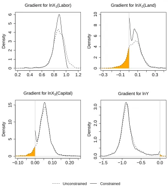
Figure 2 shows the kernel density estimates for the unconstrained and constrained distributions of the four gradients,
i.e.,∂lnD/∂lnXk,∀k= 1,2,3, and∂lnD/∂lnY, on which for each observation, a non-negativity constraint is imposed
on the first three gradients, and a non-positivity constraint is imposed on the last one. A vertical line is drawn at zero
and the shaded area highlights where the violations occur. The densities for the constrained gradients are plotted using
the Silverman reflection method for boundary correction such that the estimated densities integrate to one. It can be
seen that there are masses near zero with the constrained model for the gradients with many violations. Although very
few violations are observed for the gradient of lnX1, the unconstrained and constrained distributions of it are not close
12 We also checked whether the estimated IDF is concave in all the inputs: before the monotonicity constraints are imposed, there are 2,080
to each other. This is because the gradient of the first input is essentially a linear combination of the gradients of the
other two inputs, whose non-trivial amount of violations affect the constrained gradient of the first input.
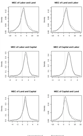
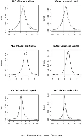
We also plot the kernel density estimates of the elasticities under the unconstrained and constrained models, as
Figure 3 and 4 illustrate. It can be seen that, in most cases, the constrained elasticities have smaller variation than their
unconstrained counterparts. This suggests that estimating an IDF satisfying its properties may improve the efficiency of
the elasticity estimates from the IDF. A vertical line is drawn at zero for a better view of the percentage of observations
whose inputs are substitutes/complements. For example, if the MEC between any two inputs is greater (less) than zero,
then these inputs are Morishima complements (substitutes). However, for both Figures, the elasticity estimates from
the unconstrained and constrained models seem to be quite close to each other. To convince the reader that significant
differences exist between the distributions, Table 3 reports thep-values from the Kolmogorov-Smirnov test for equality
of distributions for the gradients and the elasticities estimated from the unconstrained and constrained models. It can be
seen that the null of equality of distributions is rejected at the 5% level in all cases except the AEC estimates between
labor and capital.
4 Discussion
4.1 Choice of numeraire input
When it comes to estimating the IDF with some parametric functional form, e.g., Cobb-Douglas or Translog, the choice
of the normalizing input does not affect the results. However, this is generally not the case for nonparametric estimation
of the IDF.13The empirical example chooses labor input as the numeraire input when estimating the IDF. This assumes
that the labor input is endogenous. In order to see how the results change when other inputs (i.e., land or capital) are
used for normalization, we simply report the unconstrained and the constrained gradient estimates in Figures 5 and 6 in
Appendix C, which uses land and capital input as the numeraire, respectively. The elasticity plots are omitted to save
space. Although it is recommended that researchers choose an input that is endogenousa priori, the question of how to
find the most appropriate numeraire may be answered in future research.
4.2 Extensions to other representations of technology
The estimation procedure in section 2 can be easily extended to other specifications of technology. We provide two
examples here: a production and a cost function.
The production function can be written asy=B·F(X), whereyis a scalar output,B is the productivity parameter,
F(·) is an unknown function, and X is an input vector. Applying log transformation similar to (6) gives an estimable
production function: lny=f(lnX) +u, whereu= lnB is the error term. The unknown functionf(·) can be estimated
nonparametrically via kernel methods. One can also impose some desirable constraints onf(·), e.g.,∂lny/∂lnX ≥0 as
a non-negative marginal product constraint.
For the cost function, it can be written asC=λC(W, Y), whereCis the total cost,λis the productivity parameter,C(·)
is an unknown function, andWandY are input price and output vectors, respectively. Applying the log transformation and
imposing the homogeneity of degree one restriction in input price gives an estimable cost function: ln ˜C=c(ln ˜W ,lnY)+u,
where ˜C is the total cost divided by a numeraire input price, ˜W is the input price vector divided by the numeraire
input price, and u = lnλ is the error term. The cost function c(·) can be estimated using kernel methods, and some
necessary regularity constraints can be imposed on it such that (1) cost shares are constrained between zero and one:
0≤∂ln ˜C/∂ln ˜W ≤1, and (2) marginal cost is non-negative:∂ln ˜C/∂lnY ≥0.
After the regression functions are estimated under the constraints, different elasticities can then be calculated subject
to the specification of choice and data availability. See Stern (2011) for a classification scheme of different definitions of
elasticities based on primal and dual representations of technology.
4.3 Possibly endogenous regressors
It is well known that estimation of production/cost/distance functions may subject to the endogeneity problem that causes
estimation results to be biased and inconsistent. Unfortunately, the nonparametric instrumental variable (IV) estimation
is a quite young field - see Su and Ullah (2008) for a three-step estimation procedure for nonparametric simultaneous
equations models via kernel methods, and Newey and Powell (2003) for IV estimation via series approximation, among
others. It is unclear whether the CWB procedure can be seamlessly applied to the nonparametric structural models,
which may be saved for future research.
5 Conclusion
This paper uses econometric methods to estimate an input distance function (IDF) without functional form assumptions,
and imposes economic properties of the IDF on the estimated regression function via constraint weighted bootstrapping
(CWB). As a by-product, the first, second, and cross partial analytical derivatives of the estimated IDF are derived, and
thus various elasticities can be computed. Applying the proposed method to a cross-section of Norwegian forest owners,
we find that imposing the constraints eliminates the problem of economic violations in empirical work, and therefore
policy implications may be more reliable. The proposed method can be extended to other representations of technology
in a straightforward manner, and this opens the door for further empirical work to estimate models subject to economic
theory. As a future research topic, more work should be done on the unification of CWB and the nonparametric structural
modeling approach.
Acknowledgements The author would like to thank Gudbrand Lien for providing the data set, Daniel J. Henderson, Subal C. Kumbhakar, Christopher F. Parmeter, attendees at the 2011 Econometric Society North American Winter Meeting, and the two anonymous referees for
Table 1 Summary Statistics of the Variables
Symbol Variable Name Variable Description Mean Sd. Min. Max.
Y Output(m3) Harvesting level 997.4 2621.2 2 46070
X1 Labor(hours) Working hours 58.04 141.2 0.126 2632
X2 Land(hectares) Forest area cut 5.97 14.8 0.012 229
[image:12.612.121.493.227.304.2]X3 Capital(NOK) Timber stock 313740 821481 1476 16190000
Table 2 Bandwidths and Percentages of Violations
Bandwidths - ln ˜X2 ln ˜X3 lnY
- 0.2869 0.5608 0.1473
Violations ∂lnD/∂lnX1<0 ∂lnD/∂lnX2<0 ∂lnD/∂lnX3<0 ∂lnD/∂lnY >0
Percentages 0.12% 18.25% 7.08% 0.31%
1. The subscript indices are: 1 =Labor, 2 =Land, and 3 =Capital.
Fig. 1 Observation-specific Weights
Weights
Frequency
−2e−04 0e+00 2e−04 4e−04 6e−04
0
500
1000
1500
2000
2500
[image:12.612.183.409.382.601.2]Fig. 2 Kernel Density Plots of the Gradients of the IDF: Unconstrained versus Constrained
0.2 0.4 0.6 0.8 1.0 1.2
0
1
2
3
4
5
6
Gradient for lnX1(Labor)
Density
−0.3 −0.1 0.1 0.3
0
2
4
6
8
10
Gradient for lnX2(Land)
Density
−0.10 0.00 0.10 0.20
0
5
10
15
Gradient for lnX3(Capital)
Density
−1.5 −1.0 −0.5 0.0
0.0
1.0
2.0
3.0
Gradient for lnY
Density
Unconstrained Constrained
Table 3 Testing for Equality of Distributions from the Unconstrained and Constrained Models
Gradients ∂lnD/∂lnX1 ∂lnD/∂lnX2 ∂lnD/∂lnX3 ∂lnD/∂lnY -
-p-values 0.0000 0.0000 0.0000 0.0221 -
-Elasticities
M EC12 M EC13 M EC23 M EC21 M EC31 M EC32
p-values 0.0000 0.0163 0.0002 0.0000 0.0129 0.0000
AEC12 AEC13 AEC23 SEC12 SEC13 SEC23
p-values 0.0000 0.0552 0.0044 0.0000 0.0102 0.0000
1. The subscript indices are: 1 =Labor, 2 =Land, and 3 =Capital.
[image:13.612.113.501.538.657.2]Fig. 3 Kernel Density Plots of the Nonparametric MEC: Unconstrained versus Constrained
−10 −5 0 5 10 15
0.00
0.04
0.08
0.12
MEC of Labor and Land
Density
−10 −5 0 5 10 15
0.00
0.04
0.08
0.12
MEC of Land and Labor
Density
−4 −2 0 2 4
0.0
0.1
0.2
0.3
0.4
0.5
MEC of Labor and Capital
Density
−4 −2 0 2 4
0.0
0.1
0.2
0.3
0.4
MEC of Capital and Labor
Density
−4 −2 0 2 4 6
0.0
0.1
0.2
0.3
0.4
MEC of Land and Capital
Density
−10 −5 0 5 10 15
0.00
0.05
0.10
0.15
MEC of Capital and Land
Density
Fig. 4 Kernel Density Plots of the Nonparametric AEC and SEC: Unconstrained versus Constrained
−10 −5 0 5 10 15
0.00
0.04
0.08
0.12
AEC of Labor and Land
Density
−10 −5 0 5 10 15
0.00
0.04
0.08
0.12
SEC of Labor and Land
Density
−4 −2 0 2 4
0.0
0.1
0.2
0.3
0.4
AEC of Labor and Capital
Density
−4 −2 0 2 4
0.0
0.1
0.2
0.3
0.4
0.5
SEC of Labor and Capital
Density
−60 −20 0 20 40 60 80
0.000
0.010
0.020
0.030
AEC of Land and Capital
Density
−10 −5 0 5 10 15
0.00
0.10
0.20
0.30
SEC of Land and Capital
Density
References
Berndt E, Christensen L (1973) The translog function and the substitution of equipment, structures, and labor in U.S. manufacturing 1929-68. Journal of Econometrics 1(1):81–113
Berwin A, Weingessel A (2011) quadprog: Functions to solve Quadratic Programming Problems.
Blackorby C, Russell R (1981) The Morishima elasticity of substitution: Symmetry, constancy, separability, and its relationship to the Hicks and Allen elasticities. Review of Economic Studies 48:147–158
Coelli T, Perelman S (1999) A comparison of parametric and non-parametric distance functions: With application to European railways. European Journal of Operations Research 117:326–339
Cuesta R, Lovell C, Zofio J (2009) Environmental efficiency measurement with translog distance functions: A parametric approach. Ecological Economics 68:2232–2242
Du P, Parmeter C, Racine J (2013) Constrained nonparametric kernel regression: Estimation and inference. Statistica Sinica, forthcoming
F¨are R, Primont D (1995) Multi-output Production and Duality: Theory and Applications. Kluwer Academic Publishers, Boston
F¨are R, Grosskopf S, Lovell C (1985) The Measurement of Efficiency of Production. Kluwer Academic Publishers, Boston F¨are R, Grosskopf S, Lovell C (1994) Production Frontiers. Cambridge University Press, Cambridge
Grosskopf S, Hayes K, Taylor L, Webler W (1997) Budget constrained frontier measures of fiscal equality and efficiency in schooling. Review of Economics and Statistics 79:116–124
Hall P, Huang H (2001) Nonparametric kernel regression subject to monotonicity constraints. The Annals of Statistics 29(3):624–647
Hayfield T, Racine J (2008) Nonparametric econometrics: The np package. Journal of Statistical Software 27(5)
Henderson D (2009) A non-parametric examination of capital-skill complementarity. Oxford Bulletin of Economics and Statistics 71:519–538
Henningsen A, Henning C (2009) Imposing regional monotonicity on translog stochastic production frontiers with a simple three-step procedure. Journal of Productivity Analysis 32:217–229
Heshmati A, Kumbhakar S, Sun K (2013) Estimation of productivity in Korean electric power plants: A semiparametric smooth coefficient model. Working paper
Kumbhakar S, Lovell C (2000) Stochastic Frontier Analysis. Cambridge University Press, Cambridge Li Q, Racine J (2004) Cross-validated local linear nonparametric regression. Statistica Sinica 14:485–512
Li Q, Racine J (2006) Nonparametric Econometrics: Theory and Practice. Princeton University Press, Princeton Lien G, Størdal S, Baardsen S (2007) Technical efficiency in timber production and effects of other income sources.
Small-scale Forestry 6:65–78
Lovell C, Richardson S, Travers P, Wood L (1994) Resources and functionings: A new view of inequality in Australia, Springer-Verlag, Berlin, pp 787–807. Models and Measurement of Welfare and Inequality
Newey W, Powell J (2003) Instrumental variable estimation of nonparametric models. Econometrica 71(5):1565–1578 Parmeter C, Sun K, Henderson D, Kumbhakar S (2013) Estimation and inference under economic restrictions. Journal
of Productivity Analysis, forthcoming
R Development Core Team (2011) R: A Language and Environment for Statistical Computing. R Foundation for Statistical Computing, Vienna, Austria
Rambaldi A, Doran H (1997) Applying linear time-varying constraints to econometric models: With an application to demand systems. Journal of Econometrics 79(1):83–95
Ray S (2003) Measuring scale efficiency from the translog multi-input, multi-output distance function. Department of Economics, University of Connecticut, no. 2003-25, Working papers
Ryan D, Wales T (2000) Imposing local concavity in the translog and generalized Leontief cost functions. Economics Letters 67:253-260
Shephard R (1953) Cost and Production Functions. Princeton University Press, Princeton
Shephard R (1970) Theory of Cost and Production Functions. Princeton University Press, Princeton
Stern D (2011) Elasticities of substitution and complementarity. Journal of Productivity Analysis 36(1):79–89
Su L, Ullah A (2008) Local polynomial estimation of nonparametric simultaneous equations models. Journal of Econo-metrics 144(1):193–218
Terrell D (1996) Incorporating monotonicity and concavity conditions in flexible functional forms. Journal of Applied Econometrics 11(2):179–194
Appendix A
In order to obtain the derivative of the distance function with respect to each input in level form, we start from the equation in log
form:
lnD(X, Y) = lnX1+m(ln ˜X2, . . . ,ln ˜XK,lnY1, . . . ,lnYQ)
where ln ˜Xk= lnXk−lnX1,∀k= 2, . . . , K.
∂lnD ∂lnX1
= 1−
K
∑
k=2 ∂m ∂ln ˜Xk
∂lnD ∂lnXk
= ∂m
∂ln ˜Xk
,∀k= 2, . . . , K
∂2lnD ∂lnX2 1
=−
K
∑
k=2 ∂2m ∂ln ˜X2
k
·∂ln ˜Xk
∂lnX1 =
K
∑
k=2 ∂2m ∂ln ˜X2
k
∂2lnD ∂lnX2
k
= ∂
2m
∂ln ˜Xk2,∀k= 2, . . . , K ∂2lnD
∂lnX1∂lnXk
=− ∂ 2m
∂ln ˜Xk2,∀k= 2, . . . , K ∂2lnD
∂lnXk∂lnXl
= ∂
2m
∂ln ˜Xk∂ln ˜Xl
,∀k, l= 2, . . . , Kandk̸=l
Once we obtain the derivatives in log form, it would be straightforward to recover the derivatives in level form.
Dk=
∂D ∂Xk
= ∂lnD ∂lnXk ·
D Xk
,∀k= 1, . . . , K
Dkk=
∂2D ∂X2
k
= ∂ 2lnD
∂lnX2
k · D X2 k + 1 Xk ( Dk−
1 Xk
D )
∂lnD ∂lnXk
,∀k= 1, . . . , K
Dkl=
∂2D ∂Xk∂Xl
= ∂
2lnD
∂lnXk∂lnXl·
D XkXl
+Dl·
1 Xk·
∂lnD ∂lnXk
Appendix B
This appendix derives the first, second, and cross partial analytical derivatives of ˆm(z) with respect to thelth continuous variablezl.
ˆ m(z) =
n
∑
i=1 Ai(z)Yi
where
Ai(z) =
K(zi−z
h
)
∑n i=1K
(
zi−z
h
)
whereYi=−lnX1i, andK(·) is a product kernel function:
K(·) =
q
∏
s=1 K
(z
si−zs
hs
)
For thelth continuous variablezl,
K (
zli−zl
hl
) =√1
2πexp (
−1
2 (
zli−zl
hl
)2)
wherehldenotes the bandwidth forzl.
∂rmˆ(z)
∂zr l = n ∑ i=1 ∂rA
i(z)
∂zr l
Yi,∀r= 1,2
∂2mˆ(z) ∂zl∂zk
=
n
∑
i=1 ∂2A
i(z)
∂zl∂zk Y
i,∀l̸=k.
Therefore, the derivatives of ˆm(z) with respect to continuouszvariables can be expressed in terms of the derivatives ofAi(z) with respect
to these variables. Specifically,
∂Ai(z)
∂zl
=(∑ T(·)
n i=1K(·)
)2
∂2A
i(z)
∂z2
l
=
∂T(·)
∂zl
(∑n i=1K(·)
)2
−2T(·)(∑ni=1K(·) ) (∑n
i=1
∂K(·)
∂zl
)
(∑n i=1K(·)
)4
∂2A
i(z)
∂zl∂zk
=
∂T(·)
∂zk (∑n
i=1K(·) )2
−2T(·)(∑ni=1K(·)) (∑ni=1∂K∂z(·) k
)
(∑n i=1K(·)
)4
where
T(·) =∂K(·) ∂zl
n
∑
i=1
K(·)−K(·)
n
∑
i=1 ∂K(·)
∂zl
∂T(·) ∂zl
= ∂ 2K(·)
∂z2
l n
∑
i=1
K(·)−K(·)
n
∑
i=1 ∂2K(·)
∂z2
l
∂T(·) ∂zk
= ∂ 2K(·) ∂zl∂zk
n
∑
i=1
K(·)−K(·)
n
∑
i=1 ∂2K(·) ∂zl∂zk
+∂K(·) ∂zl
n
∑
i=1 ∂K(·)
∂zk −
∂K(·) ∂zk
n
∑
i=1 ∂K(·)
∂zl
We can see the derivatives ofAi(z) are functions ofT(·) and its derivatives. In order to calculateT(·) and its derivatives, we need to
calculate the first, second, and cross partial derivatives ofK(·) with respect to the continuous variables:
∂K(·) ∂zl
= (
zli−zl
h2
l
) K(·)
∂2K(·) ∂z2
l
= [
(zli−zl)2−h2l
h4
l
] K(·)
∂2K(·) ∂zl∂zk
= (
zli−zl
h2
l
) ( zki−zk
h2
k
)
Appendix C
[image:19.612.125.472.151.532.2]This appendix contains kernel density plots of the gradients of the IDF when alternative inputs are chosen as the numeraire input.
Fig. 5 Kernel Density Plots of the Gradients of the IDF: Unconstrained versus Constrained∗
0.0 0.5 1.0 1.5
0.0
0.5
1.0
1.5
2.0
Gradient for ln(Labor)
Density
−0.5 0.0 0.5 1.0
0.0
0.5
1.0
1.5
2.0
Gradient for ln(Land)
Density
−0.05 0.05 0.10 0.15
0
5
10
15
Gradient for ln(Capital)
Density
−2.0 −1.5 −1.0 −0.5 0.0
0.0
0.5
1.0
1.5
Gradient for lnY
Density
Unconstrained Constrained
Fig. 6 Kernel Density Plots of the Gradients of the IDF: Unconstrained versus Constrained∗
0.0 0.5 1.0
0.0
0.5
1.0
1.5
2.0
2.5
Gradient for ln(Labor)
Density
−0.10 0.00 0.10 0.20
0
5
10
15
Gradient for ln(Land)
Density
−0.5 0.0 0.5 1.0
0.0
0.5
1.0
1.5
2.0
2.5
Gradient for ln(Capital)
Density
−2.0 −1.0 0.0 0.5
0.0
0.5
1.0
1.5
Gradient for lnY
Density
Unconstrained Constrained