Model selection and efficiency testing for normalization of cDNA microarray data

en

t

re

v

ie

w

s

re

ports

de

p

o

si

te

d r

e

sea

rch

refer

e

e

d

re

sear

ch

interacti

o

ns

inf

ormation

microarray data

Matthias Futschik

*†

_{and Toni Crompton}

‡

Addresses: *_{Institute for Theoretical Biology, Humboldt-Universität, Invalidenstraße 43, 10115 Berlin, Germany.} †_{Department of Information} Science, University of Otago, PO Box 56, Dunedin, New Zealand. ‡_{Otago School of Medical Sciences, Division of Health Science, University of} Otago, PO Box 913, Dunedin, New Zealand.

Correspondence: Matthias Futschik. E-mail: [email protected]

© 2004 Futschik and Crompton; licensee BioMed Central Ltd. This is an Open Access article: verbatim copying and redistribution of this article are per-mitted in all media for any purpose, provided this notice is preserved along with the article's original URL.

Model selection and efficiency testing for normalization of cDNA microarray data

<p>In this study we present two novel normalization schemes for cDNA microarrays. They are based on iterative local regression and opti-mization of model parameters by generalized cross-validation. Permutation tests assessing the efficiency of normalization demonstrated that the proposed schemes have an improved ability to remove systematic errors and to reduce variability in microarray data. The analysis also reveals that without parameter optimization local regression is frequently insufficient to remove systematic errors in microarray data.</p>

Abstract

In this study we present two novel normalization schemes for cDNA microarrays. They are based on iterative local regression and optimization of model parameters by generalized cross-validation. Permutation tests assessing the efficiency of normalization demonstrated that the proposed schemes have an improved ability to remove systematic errors and to reduce variability in microarray data. The analysis also reveals that without parameter optimization local regression is frequently insufficient to remove systematic errors in microarray data.

Background

Microarrays have been widely used for the study of gene expression in biological and medical research. They allow the simultaneous measurement of the expression of thousands of genes in cells. However, microarrays do not assess gene expression directly, but only indirectly by monitoring fluores-cence intensities of labeled target cDNA hybridized to probes on the arrays [1]. The first step in the analysis of microarray data is, therefore, the transformation of fluorescence signals into quantities of gene expression. This includes several data pre-processing procedures - for example, excluding artifacts and correcting for background intensities. The signals also have to be adjusted for differences in dye labeling, fluores-cence yields, scanning amplification and other systematic variability in the measurement. Although this so-called nor-malization procedure is only an intermediate step in the anal-ysis, it has a considerable influence on the final results [2]. Assessment of the efficiency of a chosen normalization method should therefore be an integral part of every normal-ization procedure.

Important and widely used microarray platforms are spotted cDNA microarrays consisting of probes that are spatially ordered on a rigid surface. Probes for cDNA arrays are gener-ally the polymerase chain reaction (PCR) products derived from cDNA clone sets and are spotted on the array using a set of pins [1]. To measure gene expression by cDNA microar-rays, RNA samples are reverse transcribed to cDNA and labeled with fluorescent dyes. The labeled target cDNA is then hybridized to the microarray probes. To control variability due to variable spot size and concentration of arrayed PCR product, cDNA microarrays arrays are generally co-hybrid-ized with two samples, one of which serves as the reference sample. The two samples for a cDNA array are labeled by dif-ferent dyes (for example, Cy5, Cy3) with distinct optical prop-erties. Pairing the signal intensities of both samples for each spot aims to eliminate the variability of the spotting proce-dure. The calculated ratio of signal intensities for each spot delivers a measure for fold changes in gene expression. How-ever, raw fluorescence ratios are frequently misleading. The corresponding fold changes might reflect experimental biases rather than changes in gene expression.

Published: 30 July 2004 Genome Biology 2004, 5:R60

Received: 5 December 2003 Revised: 11 May 2004 Accepted: 28 June 2004 The electronic version of this article is the complete one and can be

A well known experimental bias for cDNA arrays is the so-called dye bias, referring to the systematic error that origi-nates from using two different dyes. Dye bias is most appar-ent in self-self hybridization experimappar-ents, in which idappar-entical samples are labeled by two different dyes and hybridized on the same array. It could be expected that ratios of spot signal intensities vary around one. However, intensity-dependent deviations from such behavior have frequently been observed [3,4]. These deviations can be related to a variety of experi-mental factors such as differing labeling efficiencies, fluores-cence quantum yields, background intensities, scanning sensitivity, signal amplification and total amount of RNA in the samples [1,4,5]. Besides intensity-dependent dye bias, other types of dye bias have been reported [5-8].

Normalization aims to correct for systematic errors in micro-array data. A variety of normalization methods have been proposed for two-color arrays (for a recent review see [9]). One of the first methods proposed to correct for dye bias was global linear normalization, which assumes that the total flu-orescence in both channels is equal [10]. On the basis of this assumption, a normalization constant can be derived and used to adjust the fluorescence intensities of the two chan-nels. However, recent reports have shown that this procedure is insufficient to correct for nonlinear dependence of spot intensities and fluorescence ratios [4,6,11]. Several normali-zation methods have been developed to overcome this short-coming of global normalization [6-8,11]. They commonly regress fluorescence ratios with respect to spot intensities in a nonlinear fashion. Some of these local regression methods have been further extended to correct for spot location-dependent dye bias [6,7].

Although nonlinear normalization procedures have been able to reduce systematic errors, an optimal adjustment of these normalization models to the data has not been discussed. Current methods are based on default parameter values and leave it up to the researcher to adjust the normalization parameters. Instructions on how to optimize parameter set-tings are generally not given. Optimization of parameters is, however, crucial for the normalization process. We show in our study that systematic errors in cDNA microarray data exhibit a large variability between, and even within, experi-ments. This requires an adjustment of the model parameters to the data. A set of normalization parameters of fixed value is frequently insufficient to correct experimental biases.

In this study we introduce two normalization schemes based on iterative local regression and model selection. The under-lying relations between experimental variables and gene-expression changes were derived from an explicitly formu-lated hybridization model. Both normalization schemes aim to correct for intensity- and location-dependent dye bias in cDNA microarray data. For model selection, we applied gen-eralized cross-validation (GCV), which has computational advantages compared to standard cross-validation. The

effi-ciencies of correction for dye bias of different normalization schemes were compared using permutation tests for two independently generated cDNA microarray datasets. Several statistical measures were used to assess the variability and reproducibility of results obtained by different normalization methods. Finally, the normalized fold changes of multiple genes were compared to externally validated fold changes for a third microarray experiment.

Results

Hybridization model

A first step in the analysis of microarray data is the develop-ment of a hybridization model relating intensity of fluores-cent signals to mRNA abundance. The model should describe the influence of experimental parameters on the data varia-bility and include error terms. Explicitly modeling the rela-tion between signal intensities and changes in gene expression can separate the measured error into systematic and random errors. Systematic errors may be corrected in the normalization procedure, whereas random errors cannot be corrected, but have to be assessed by replicate experiments. Removal of systematic errors is important, as they limit the accuracy of the measurement, whereas random errors limit its precision.

Our hybridization model applies to two-color arrays com-monly consisting of a red (Cy5) and green (Cy3) fluorescence channel. The model relates the measured spot fluorescence intensity to changes in the labeled transcript abundances in which we are interested. Its explicit derivation can be found in Materials and methods. Specifically, the model relates the ratios I_r/I_g of spot signal intensities (I_r/g, spot fluorescence intensity in red/green channel) with the ratios T_r/T_g of labeled transcript abundance (T_r/g, abundance of transcript labeled by red/green dye). The relation has the following form:

M - κ(J) = D + ε (1)

where M is the log fluorescence intensity ratio (M = log₂I_r/I_g), D is the logged ratio of transcript abundance (D = log₂T_r/T_g) and εrepresents the random error. The term κis an additive factor that can depend on a set of experimental variables J, for example, spot intensity and location. In our model, κ(J) can be seen as a term for systematic errors. Using Equation (1), we can derive D from M up to the random error term ε once we know κ(J). The factor κ(J) is generally calibrated by exploiting Equation (1). Depending on the assumptions about the experiment, we can proceed with different normalization methods.

comm

en

t

re

v

ie

w

s

re

ports

refer

e

e

d

re

sear

ch

de

p

o

si

te

d r

e

sea

rch

interacti

o

ns

inf

ormation

from the signal ratios assuming symmetry of the logged fold changes D and error term ε. The factor κ(J) can then be calcu-lated by a local regression of M with respect to the fluores-cence intensity. This procedure can be performed using all or a selected subset of genes and is frequently called intensity-dependent normalization. In the experiments analyzed, we found that the measured spot intensity ratios showed not only intensity-dependent, but also spatial bias across the array. We introduce, therefore, two normalization schemes that simultaneously correct for dye bias due to intensity and spa-tial location.

Normalization schemes

Two normalization schemes were developed to determine the normalization factor κ(J) in the hybridization model (Equa-tion (1)). They are based on iterative local regression and incorporate optimization of model parameters. Local regres-sion is performed using LOCFIT, which is based on the same computational ideas as the popular lowess method [12,13]. However, it differs from lowess in that its implementation offers more flexibility to the user. For local fitting, LOCFIT (as well as lowess) requires the user to choose a smoothing parameter α that controls the neighborhood size h. The parameter αspecifies the fraction of points that are included in the neighborhood and thus has a value between 0 and 1. Larger αvalues lead to smoother fits. In addition, the setting of scale parameter s is necessary for a local regression with two or more predictor variables. These parameters provide the scales of the predictor variables for the fitting procedures. The parameter s can be of arbitrary value.

For normalization by LOCFIT, therefore, model parameters α and s have to be chosen. The choice of model parameters for local regression is crucial for the efficiency and quality of nor-malization. To optimize the model parameters, we use a cross-validation procedure. Because conventional leave-one-out cross-validation becomes computationally prohibitive for this task, we used GCV, which approximates the leave-one-out method [14]. GCV is computationally less expensive to perform as it does not require multiple constructions of regression models based on partial data, as standard cross-validation does.

Both normalization schemes aim to correct for systematic errors linked to spot intensity and location. The first proce-dure leaves the scale of log intensity ratios M unchanged, whereas the second procedure includes an adjustment of the scale of M. The notation is as follows: A = 0.5 (log₂ I_r + log₂I_g), which is the geometric mean of the fluorescent intensities of both channels; X is the spot location on the array in the X direction; Y is the spot location on the array in the Y direction; α_A is the smoothing parameter for local regression of M with respect to A; α_XY is the smoothing parameter for local regres-sion of M with respect to spatial coordinates X and Y; s_Y is the scale parameter allowing a different amount of smoothing in the Y direction compared to smoothing in the X direction.

Optimized local intensity-dependent normalization (OLIN)

For a set of smoothing parameter α_A, local regression of M with respect to A is performed, generating a set of regression models. Then, the regression models are compared by GCV. The model with resulting in the minimum GCV criterion is chosen. The optimal fit (A) corresponds to a normal-ization factor κ(A) in Equation (1). (A) is subtracted from M, generating an intensity normalized M: M ← M (A). For a set of smoothing parameter α_XY and a set of scale parameter s_Y, local regression of M with respect to X and Y is performed. The resulting models are compared by GCV. The optimal fit (A) corresponds to a normalization factor κ(X,Y) in Equation (1). (A) is subtracted from M generating a spatially normalized M: M ←M - (A). The steps above are repeated, unless the maximal number of iterations N is reached. If the maximal number of iterations is reached, M is the normalized log intensity ratio.

Optimized scaled local intensity-dependent normalization (OSLIN) First, OLIN is performed. Then, for a set of smoothing param-eter α and a set of scale parameter s, local regression of abs(M) with respect to X and Y is performed. The resulting models are compared by GCV. The model with α* and s* pro-ducing the minimum GCV criterion is chosen and an optimal

fit produced. M is locally scaled by : M' ←M/ . The global scale of M' is adjusted, so that total varia-tion of M remains constant:

M" is the normalized log intensity ratio.

We applied our hybridization model and normalization schemes to data from two independent spotted cDNA micro-array experiments. In the first experiment, gene expression in two colon cancer cell lines (SW480/SW620) was compared [15]. The SW480 cell line was derived from a primary tumor, whereas the SW620 cell line was cultured from a lymph-node metastasis of the same patient. Sharing the same genetic background, these cell lines serve as an in vitro model of can-cer progression [16]. The comparison was direct, that is with-out using a reference sample. cDNA derived from SW480 cells was labeled by Cy3; cDNA derived from SW620 was labeled by Cy5. The SW480/620 experiment consisted of four technical replicates. In the second experiment (apo AI), gene expression in tissue samples from eight apo AI knock-out and eight control mice was studied [17,18]. Cy5-labeled cDNA from each tissue sample was co-hybridized with a Cy3-labeled reference sample consisting of pooled cDNA from the control

α*_A

M

A

α*

M

A

α*

M

A

α*

M

XY Ys

α* *

M

XY Ys

α* *

M

XY Ys

α* *

M_αabs* *_s M_αabs* *_s

M_αabs* *_s

′′ ← ′

( )

′

( )

M M M

M

* var

mice. Hence, a total of 16 cDNA microarrays comprise the apo AI experiment. Technical replicates were missing. Further information regarding the experiments can be found in the Materials and methods section.

The effects of the normalization schemes are illustrated here for a chosen microarray (slide 3) of the SW480/620 experi-ment. The first step of normalization is, however, the identi-fication of systematic experimental variability in the data.

Identification of systematic errors: intensity-dependent and location-intensity-dependent dye bias

Visual inspection of different plot representations of the data pointed to two major types of systematic errors: intensity-dependent and location-intensity-dependent dye bias. Although visual inspection lacks the stringency of statistical analysis, it pro-vides an important first tool to detect artifacts in microarray data.

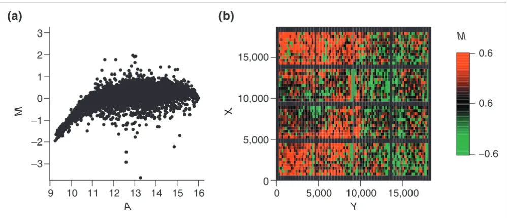
Popular representations are plots of Cy5 (I_r) versus Cy3 (I_g) intensities on linear or log scale. To illustrate the effect of the normalization procedures, however, the use of transformed log intensities is preferable [4]. In so-called MA-plots the log ratio M = log₂(I_r/I_g) = log₂(I_r) -log₂(I_g) is plotted against the mean log intensities A = 0.5(log₂(I_r) + log₂(I_g)) Although MA-plots are basically only a 45° rotation with a subsequent scal-ing, they reveal intensity-dependent patterns more clearly than the original plot. MA-plots also introduce a measure for the spot intensity A, which was used in our normalization schemes. Figure 1a presents the MA-plot for the raw data of

slide 3. Clearly, it shows a general nonlinear dependence of log ratios M on spot intensity A. For low intensities, M is biased towards negative values, which is generally the case for arrays of the SW480/620 experiment. This is contrasted by MA-plots of the apo AI experiment, where log ratios are gen-erally biased towards positive values for low spot intensities (see Figure 3 in additional data file 1). The differing character-istics of this dye bias may be caused by differences in labeling or scanning protocol used in the two experiments. In addition to standard MA-plots, we found that it can be favorable to smooth the MA-plot by calculating the average value of M within a moving window along the intensity scale. Such A-plots frequently display the dependence of M on A more clearly (see Figure 2 in additional data file 1). As well as inten-sity-dependent bias, the MA-plot in Figure 1 also reveals sat-uration effects for spots of high intensities. A substantial saturation is indicated by arrow-shaped distributions of spots in MA-plots. Such effects are caused by the limited dynamical range of M due to the scanner detection limit of 216 _{- 1 units.}

A more detailed analysis of saturation and how it affects MA-plots can be found in [19]. Ratios corresponding to spots with saturation in one or both channels should be treated with care, as a recovery of the unsaturated intensities is generally not possible (see the Hybridization model section in Materi-als and methods). Therefore, normalization cannot correct for such saturation effects. To avoid this difficulty, saturation should be prevented by adjustment of scanning parameters. Alternatively, a multiple scanning procedure can be applied [20].

M

Intensity and spatial distribution of raw log intensity ratios M of slide 3 of the SW480/620 experiment

Figure 1

Intensity and spatial distribution of raw log intensity ratios M of slide 3 of the SW480/620 experiment. (a) The MA-plot indicates a strong bias towards the Cy3 channel for low spot intensities A. (b) The spatial MXY-plot shows uneven distribution of positive M (red squares) and negative M (green squares). The columns with consistently negative M correspond to empty control spots. The axis labels X and Y refer to the spot location as determined by the QuantArray scanning software.

15,000 3

2

1

0

−1

−2

−3

10,000

0.6

0.6

−0.6 5,000

0

0 5,000 9 10 11 12 13

A Y

X

M

M

14 15 16 10,000 15,000

comm

en

t

re

v

ie

w

s

re

ports

refer

e

e

d

re

sear

ch

de

p

o

si

te

d r

e

se

a

rch

interacti

o

ns

inf

o

rmation

Less frequent than the I_r - I_g-plots or MA-plots is the repre-sentation of log ratios based on the corresponding spot loca-tion. This type of plot, termed here a MXY-plot, offers, however, a valuable tool for assessing the quality of hybridi-zation as well as the subsequent normalihybridi-zation. MXY-plots show the log ratios M with respect to the spot location on the

array. Positive M values are represented as red squares, whereas negative M values are shown as green squares. The MXY-plot for the raw data of slide 3 is shown in Figure 1b. Large areas show a tendency towards positive M (for exam-ple, the lower left side). For slides of both experiments, MXY-plots point to the existence of spatial bias. Whereas spatial Intensity and spatial distribution of log ratios for local intensity-dependent normalization (LIN) with default model parameters

Figure 2

Intensity and spatial distribution of log ratios for local intensity-dependent normalization (LIN) with default model parameters. (a) The residuals of the local regression are well balanced around zero in the MA-plot. (b) Patterns of spatial bias are still apparent in the MXY-plot, whereas the lines of negative M corresponding to empty spots disappeared as a result of the intensity-dependent normalization.

Intensity and spatial distribution of log ratios for optimized local intensity-dependent normalization

Figure 3

Intensity and spatial distribution of log ratios for optimized local intensity-dependent normalization. (a) MA-plot; (b) MXY-plot. Both plots indicate no apparent bias for log ratio M with respect to the intensity A or the spot location (X,Y). Note, however, that the MXY-plot shows areas of differing brightness corresponding to areas of differing variability of M. Regions with large abs(M) appear, therefore, brighter than regions with small abs(M). For example, the variance of M seems to be larger around spot location (X = 2,500, Y = 16,000) than round the location (X = 7,000, Y = 3,000).

15,000 3

2

1

0

−1

−2

−3

10,000

0.6

0.6

−0.6 5,000

0

0 5,000 9 10 11 12 13

A Y

X

M

M

14 15 16 10,000 15,000

(a)

(b)

15,000 3

2

1

0

−1

−2

−3

10,000

0.6

0.6

−0.6 5,000

0

0 5,000 9 10 11 12 13

A Y

X

M

M

14 15 16 10,000 15,000

bias was variable across different slides of the SW480/620 experiment, it was more consistent for slides of the apo AI experiment (see Figures 4 and 5 in additional data file 1). As an alternative to MA-plots, the average value of neighbor-ing spots can again be used instead of M for plotting. These XY-plots frequently display spatial artifacts more clearly than MXY-plots (see Figure 2 in additional data file 1).

In contrast to intensity-dependent dye bias, the origin of spa-tial bias is less clear. Possible reasons for the observed spaspa-tial bias might be spatial inhomogeneities of hybridization, une-ven slide surfaces or unbalanced scanning procedures [1]. Schuchhardt et al. [5] and Yang et al. [6] suggested a ratio bias linked to the use of different pins. In this case, a block-wise bias would be apparent, which we did not observe. In our experiment, the spatial dye bias seemed to be continuous across arrays. Of course, one explanation for the uneven spa-tial distribution is that it reflects actual biological variability. For example, the lower left side of the array in Figure 1b could be enriched with spots corresponding to upregulated genes. This, however, seems to be unlikely, as the print order of spots in the SW480/620 experiment did not follow functional cat-egories of genes. Even if genes are grouped on the used micro-titer plates on the basis of their functions, the spotting procedure used for cDNA arrays leads to an even distribution of those genes across the array. Moreover, the spatial patterns of log ratios M differed between replicate arrays of the SW480/620 experiment. If they were specific for the print layout of the probes, similar patterns in all arrays would be expected. Other arguments also point against a biological source of the observed intensity-dependent and spatial dye bias for the experiments analyzed here. First, log ratios close to zero can be expected for empty control spots in the SW480/620 experiment. However, a large number of empty control spots with low fluorescence signals due to nonspecific hybridization had consistently large negative log ratios. They would be falsely detected as significant if no data normaliza-tion was applied [15]. Second, only a small number of genes are expected to be differentially expressed in the apo AI experiment [6]. Therefore, both MA- and MXY-plots should show log ratios close to zero for the vast majority of spots.

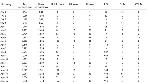
As well as visual inspection, we used permutation tests to detect intensity-dependent and spatial dye bias. The tests determined the significance of observing a median log ratio within a spot intensity or location neighborhood as intro-duced in Materials and methods. The number of neighborhoods with significant for the false discovery rate (FDR) = 0.01 is shown in Tables 1 and 2. For spot-inten-sity neighborhoods, a symmetrical window of 50 spots was chosen, whereas a 5 × 5 window was chosen as the spot-loca-tion neighborhood. For slide 3 of the SW480/620 experi-ment, testing the dependency of log ratio M on spot intensity A revealed that 1,138 spot neighborhoods (or 27% of all neigh-borhoods) had a significantly large positive or negative

median log ratio. Testing for location-dependent dye bias, 837 neighborhoods (20%) were detected as significant.

A simple but popular method for normalizing cDNA microar-ray data is global linear normalization. However, linear nor-malization leads only to a vertical shift along the M-axis in the plots (see Figure 1 in additional data file 1). Thus, the inten-sity- and location-dependent bias remained apparent. This was confirmed by the results of the permutation tests: 988 spot-intensity and 815 spot-location neighborhoods were detected as significant. This shows that linear normalization was insufficient to remove the observed dye and spatial bias

Local intensity-dependent normalization

Inspection of the MA- and MXY-plots showed that the rela-tions between log ratio M and spot intensity A and between log ratio M and spot location (X, Y) are nonlinear. In our hybridization model, the normalization factor κshould there-fore be a function of A as well as X and Y:

M_i-κ(A,X,Y) = D_i + ε_i (2)

If we combine the logged fold change D_i and error term ε_i to a random variable ζ_i which is assumed to be symmetrical dis-tributed around zero, we get

M_i = κ(A,X,Y) + ζ_i (3)

Since this relation is of the same form as Equation (10) (see below), we can apply a local regression model to capture the intensity and location dependence of M. The residuals of the regression provided the logged fold changes D up to an error term and were used for the MA- and MXY-plots. The assump-tion that variable ζ_i is symmetrically distributed has to taken with caution, as it is based on two requirements: most genes arrayed are not differentially expressed or the numbers of up-and downregulated genes are similar; up-and the spotting proce-dure did not generate an spatial accumulation of up- or down-regulated genes in localized areas on the array. Both requirements have to be assessed for each experiment indi-vidually. From the discussion in the previous section, we believe that both requirements are fulfilled for the datasets analyzed in this study.

To examine the influence of model selection on final normal-ization results, we first conducted the same normalnormal-ization procedure as OLIN but without parameter optimization by GCV. Instead, we used default values for the model parame-ters. This provides a 'baseline' model termed LIN, which we compared to the optimized models OLIN and OSLIN. A default value of 0.5 was used for fitting parameters α_A and α_XY. The scaling parameter s_Y was set to 1. The iterative pro-cedure was maintained for LIN to ensure self-consistency of results, as we regress stepwise with respect to intensity A and location (X,Y). The number of iterations was set to three. The results are displayed in Figure 2. The MA-plot data normal-M

M

M

comm

en

t

re

v

ie

w

s

re

ports

refer

e

e

d

re

sear

ch

de

p

o

si

te

d r

e

se

a

rch

interacti

o

ns

inf

o

rmation

ized by LIN showed that the residuals are centered around zero (Figure 2a). The considerable bias of log ratios M for low spot intensities A was removed. This was confirmed by testing normalized log ratios for intensity-dependent bias. No spot-intensity neighborhood with a significant median log ratio was detected (Table 1).

However, careful inspection of the MXY-plot shows that the spatial bias was only partially removed, as spatial patterns

were still visible (Figure 2b). The permutation tests also revealed that the distribution of M is not balanced across the array. Seventy-eight spots had neighborhoods with a signifi-cant large median log ratio (Table 2). The result indicates that local (spatial) features exist in the data, which were not appropriately fitted by LIN. This points to the importance of model parameter optimization, especially for location-dependent normalization.

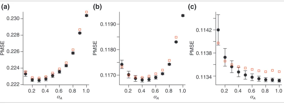
Comparison of GCV and fivefold cross-validation

Figure 4

Comparison of GCV and fivefold cross-validation. The relation between prediction mean square error (PMSE) and smoothing parameter αA is shown for the three iterations (a-c) in the OLIN procedure applied to slide 16 of the apo AI experiment. The fivefold cross-validation was conducted for five random splits of the data. Mean values and standard errors of PMSE estimates are represented as black circles and error bars. PMSE estimates by GCV are represented by red squares. Generally, these estimates lie within the error margin of PMSE produced by fivefold cross-validation. The GCV-optimized value of αA was 0.3 for the first (a), 0.4 for the second (b), and 1.0 for the third (c) iteration.

Intensity and spatial distribution of log ratios M for optimized scaled local intensity-dependent normalization

Figure 5

Intensity and spatial distribution of log ratios M for optimized scaled local intensity-dependent normalization. (a) MA-plot. (b) MXY-plot. This shows that the variability of log ratios is even across slide 3 of the SW480/620 experiments.

0.2 0.4 0.6 0.8 1.0 0.2 0.4 0.6

αA αA αA

0.8 1.0 0.2 0.4 0.6 0.8 1.0

PMSE

PMSE PMSE

0.1134 0.1138 0.1142

0.1170 0.1180 0.1190

0.222 0.224 0.226 0.228 0.230

(a)

(b)

(c)

15,000 3

2

1

0

−1

−2

−3

10,000

0.6

0.6

−0.6 5,000

0

0 5,000 9 10 11 12 13

A Y

X

M

M

14 15 16 10,000 15,000

Optimized local intensity-dependent normalization To improve the efficiency of normalization, we conducted OLIN with model optimization by GCV. Three parameters (α_A, α_XY, s_Y) had to be optimized during each iteration. Parameters (α_A, α_XY) determine the proportion of data used for local intensity-dependent and spatial regression of log ratio M, respectively. They control the smoothness of fits. Choosing accurate parameter α_A and α_XY is crucial for the quality of the regression. Too large parameter values result in a poor fit, where local data features are missed; too small val-ues lead to overfitting of the data. Two extreme cases illustrate the importance of parameters α_A and α_XY. If we choose a value of 1, all data points are included in the local regression. Although the weight function tricube W used by LOCFIT forces larger weights to be put on neighboring points, the fit becomes increasingly linear. The other extreme case is the use of a diminutive parameter value, which leads to fitting of every point independently of its neighborhood. Overfitting of the data occurs and the residuals are subsequently under-estimated. Besides smoothing parameters α_A and α_XY, OLIN demands the setting of scaling parameter s_Y. This is especially important if spatial patterns of log ratio M vary on differing scales across the array. GCV was used to determine the

optimal setting of model parameters. For α_A and α_XY, a parameter range of 0.1 to 1 was tested. For s_Y, values between 0.05 and 20 were compared. The number of iterations was set again to three. If more iterations were performed only minor changes in the outcome of normalization were observed, indi-cating that self-consistency of normalization was reached.

Inspection of the MXY-plot revealed that the optimized local intensity-dependent normalization was able to correct for the spatial bias (Figure 3b). Spots with positive and negative log ratio M were evenly distributed across the slide. The patterns of spatial bias across the array were no longer apparent. Sim-ilarly, the residuals were well balanced around zero in the MA-plot (Figure 3a). The results of the statistical tests under-lined these findings. No significant neighborhoods were found on testing for intensity-dependent dye bias and only one neighborhood remained significant on testing for spatial bias (Tables 1 and 2).

The GCV procedure only approximates the prediction error of standard cross-validation. To test if this approximation is accurate for the microarray data analyzed, we compared the GCV estimates with the estimates produced by fivefold

cross-Table 1

Number of significant spot neighborhoods on the intensity scale for arrays of the experiments analyzed

Microarray No

normalization

Linear normalization

Global lowess P-lowess S-lowess LIN OLIN OSLIN

SW 1 596 580 2 5 7 39 12 0

SW 2 1,090 1,080 0 0 0 52 0 0

SW 3 1138 988 0 0 0 0 0 0

SW 4 745 655 0 9 4 0 12 0

Apo 1 1,748 1,810 18 0 0 26 0 0

Apo 2 2,739 2,683 16 17 26 24 0 0

Apo 3 3,479 3,559 52 30 15 0 1 0

Apo 4 2,122 2,184 1 17 22 0 0 11

Apo 5 3,885 3,886 100 13 11 94 0 0

Apo 6 3,540 3,555 0 0 0 114 0 0

Apo 7 3,725 3,724 0 0 7 0 0 0

Apo 8 3,253 3,296 66 0 0 507 0 0

Apo 9 1,040 1,044 114 0 0 455 0 0

Apo 10 1,554 1,575 0 0 0 45 0 0

Apo 11 2,903 2,889 5 34 35 2 0 0

Apo 12 3,536 3,543 14 0 0 47 0 0

Apo 13 2,819 2,901 132 12 3 354 4 0

Apo 14 2,291 2,342 313 0 12 484 64 4

Apo 15 3,050 3,034 95 36 0 164 0 0

Apo 16 1,338 1,374 159 0 12 918 0 0

Spot neighborhoods are found significant if the median log ratio M has larger positive and negative value than expected from random order of spots

comm

en

t

re

v

ie

w

s

re

ports

refer

e

e

d

re

sear

ch

de

p

o

si

te

d r

e

se

a

rch

interacti

o

ns

inf

o

rmation

validation. Although GCV is considerably less ally demanding, it reproduces estimates of the computation-ally intensive fivefold cross-validation genercomputation-ally well (see Figure 4). The α_A values selected by GCV ranged from 0.1 to 0.7 for the SW480/620 experiment and between 0.2 and 0.7 for the apo AI experiment. Smaller values produced overfit-ting of data; larger values yielded underfitoverfit-ting. For the third iteration, an α_A value of 1 was generally selected, resulting in an approximately linear fit. Optimization of spatial regression parameters α_XY and s_Y showed a more complex behavior and varied between experiments and slides.

Although OLIN leads to an even spatial distribution of posi-tive and negaposi-tive log ratios M, visual inspection of Figure 3b indicates that the variability of log ratios might be unbalanced across the array. This can also be assessed by permutation tests. In the same manner as for spatial bias detection, we derived the number of neighborhoods with significant median abs(M) values. The results can be found in Table 1 of additional data file 1. For slide 3 of SW480/620 experiment, 25 spot neighborhoods were detected as significant using FDR = 0.01. Therefore, it may be favorable to adjust the scale of log ratios M locally.

Optimized scaled local intensity-dependent normalization

If we can assume that the variability of log ratios M should be equal across the array, local scaling of M can be performed. As in the previous section, the validity of these assumptions has to be carefully checked for each array analyzed. The underly-ing requirement is again random spottunderly-ing of arrayed genes. As we believe this requirement is fulfilled for our experi-ments, we applied optimized local scaling within the OSLIN scheme. The local scaling factors are derived by optimized local regression of the absolute log ratio M. The range of regression parameters tested by GCV is (0.1,1) for smoothing parameter α and (0.05,20) for scaling parameter s_Y. The resulting MA- and MXY-plots for slide 3 are presented in Fig-ure 5. The variability of log ratios M appears to be even across the array. This is consistent with the result of the correspond-ing permutation test: No significant spot neighborhood was detected (see Table 2 in additional data file 1).

Slide-wise comparison of normalization schemes The normalization methods proposed in this study yielded different results. To choose the optimal method, the efficiency of normalization in removing systematic errors has to be

Table 2

Number of significant spot neighborhoods across the spatial layout of the arrays analyzed

Microarray No

normalization

Linear normalization

Global lowess P-lowess S-lowess LIN OLIN OSLIN

SW 1 1,500 1,483 1,625 214 220 106 0 0

SW 2 808 831 1,068 218 113 67 0 0

SW 3 874 815 723 126 96 78 1 0

SW 4 741 757 846 76 43 49 0 0

Apo 1 1,173 1,196 1,276 913 491 755 100 1

Apo 2 521 518 801 176 74 221 3 0

Apo 3 562 576 706 334 79 258 0 0

Apo 4 770 771 1,058 177 14 176 2 0

Apo 5 670 648 844 357 222 381 5 0

Apo 6 432 432 1,003 129 106 296 10 0

Apo 7 516 526 1,258 186 88 194 17 0

Apo 8 850 833 1,202 684 342 458 61 9

Apo 9 1,596 1,621 1,780 1,105 644 798 21 5

Apo 10 707 711 896 261 108 279 3 0

Apo 11 504 484 1,306 166 87 258 11 0

Apo 12 1,313 1,323 1,144 425 288 370 12 17

Apo 13 1,357 1,368 1,155 653 394 568 41 0

Apo 14 862 1,005 987 273 108 272 82 0

Apo 15 733 743 1,004 588 241 502 97 0

Apo 16 942 985 1,347 786 333 470 47 0

compared. As well as the methods presented above, we included three previously proposed normalization methods based on lowess regression and implemented in the Biocon-ductor software package [6,21]: global intensity-dependent normalization (global lowess) which regresses log ratios M with respect to spot intensity A; within print-tip group nor-malization (P-lowess) which regresses M with respect to A for every print-tip group independently; and scaled within-print-tip group normalization (S-lowess), which scales log ratios M for each print-tip group after P-lowess is applied. Note that the smoothing parameter αfor these methods is constant and the default value of 0.4 was used.

The results of the comparison are examined in detail here for slide 1 of the apo AI experiment. The corresponding MA-plots can be found in Figure 3 in additional data file 1. Although lin-ear normalization led to an overall balanced distribution of M, it was insufficient to remove the intensity-dependent dye bias. The nonlinear methods applied were generally able to correct for intensity-dependent bias. Figure 6 presents the MXY-plots for slide 1 of the apo AI experiment. For global lin-ear normalization, the corresponding MXY-plot indicates that this method is insufficient to remove spatial artifacts on the array. Easily noticeable stripes of positive or negative log ratio remained. Spots near the right edge of slide 1 show a considerable bias towards positive log ratios. Note that these spatial patterns do not correlate with the sub-grid defined by the 4 × 4 print-tips. Application of global lowess normaliza-tion failed to remove these spatial artifacts. This can be expected, as the global lowess method does not incorporate any special normalization. A reduction in spatial bias can be seen for P-lowess, S-lowess and LIN which all include spatial normalization. However, spatial patterns remain prominent. For P-lowess and S-lowess, this indicates that they are not able to correct for spatial artifacts that are not correlated with print-tip groups. For LIN, it points to underfitting of the data, and thus the necessity of parameter optimization. Inspection of the MXY-plots for OLIN and OSLIN confirms that this was indeed the case: location-dependent dye bias was absent in both plots. In addition, the MXY-plot for OSLIN shows an even variability of log-ratios across the array.

To assess the validity of the findings based on visual inspec-tion, the efficiency of normalization was also examined by permutation tests (Tables 1 and 2). For 1,750 spots, a signifi-cant intensity neighborhood was detected if no normalization was applied. Most significant spot neighborhoods could be found at low spot intensities. Global linear normalization even led to a slight increase in number of significant neigh-borhoods. All methods incorporating local intensity-depend-ent normalization performed with similar efficiency. For P-lowess, S-P-lowess, OLIN and OSLIN, no spots with significant neighborhoods were detected, whereas 18 remained for glo-bal lowess and 15 for LIN. Testing for spatial bias, we found 1,173 spot neighborhoods with significant large log ratios if no normalization was applied. Linear and global lowess

normalization increased the number of spatially biased neighborhoods. P-lowess, S-lowess and LIN reduced the number of significant neighborhoods, although only with a limited efficiency (P-lowess, 913; S-lowess, 491; LIN, 755). A considerable reduction of spatial bias was achieved by OLIN: 100 neighborhoods were detected as significant after normal-ization. OSLIN showed the best performance. Only one spot neighborhood remained significant.

Besides giving an indication about the efficiency of normali-zation, the testing procedure applied also enabled us to iden-tify regions of dye and spatial bias. This is illustrated in Figure 7. Spots are represented by red squares if their neighborhood has a significant positive median log ratio M. Correspond-ingly, spots are represented by green squares if their neigh-borhood has a significant negative median log ratio. By varying the level of FDR, the grade of significance can be assigned. This approach enables a stringent localization of significant experimental bias. Figure 6 shows, for example, that spots close to the right edge are especially affected by spatial artifacts.

Although the number of significant neighborhoods varied between slides and experiments, the results of the comparison undertaken for slide 1 of the apo AI experiment remain generally valid for the other slides analyzed (Tables 1 and 2). Linear normalization was unable to remove intensity-dependent and location-intensity-dependent dye bias. Global lowess corrected for intensity-dependent, but not for spatial bias. P-lowess, S-lowess and LIN performed well in the correction for intensity-dependent bias, but were less efficient in correcting for spatial dye bias. For most slides, OLIN and OSLIN showed the highest efficiencies in removing both types of systematic error.

An alternative, and computationally less expensive, way to examine intensity- and location-dependent bias is the corre-lation of the log ratio M with average in the spot's neigh-borhood [5]. Assuming that log ratios of neighboring spots are uncorrelated, a correlation close to zero can be expected. A large positive correlation, however, indicates the existence of bias. Successful normalization, therefore, should remove the correlation of log ratios of neighboring spots. We con-ducted this type of correlation analysis for each array inde-pendently. Spot intensity and location neighborhoods were defined as before. The results can be found in Tables 2 and 3 of additional data file 1. We present and discuss here the aver-age correlation coefficients for the two experiments analyzed (Table 3). For the SW480/620 experiment, the average Pear-son correlation of a spot's log ratio M and the median log ratio of spots in its intensity neighborhood was 0.50. Whereas linear normalization lead to exactly the same correlation coef-ficient, the nonlinear methods compared yielded a correla-tion coefficient close to zero. Correlating the log ratio M of spots with the median log ratio of their spatial neighbor-hood resulted in a correlation of 0.53 for raw data. Linear

nor-M

M

comm

en

t

re

v

ie

w

s

re

ports

refer

e

e

d

re

sear

ch

de

p

o

si

te

d r

e

se

a

rch

interacti

o

ns

inf

o

rmation

malization again yielded the same correlation. Global lowess slightly increased the correlation. P-lowess, S-lowess and LIN achieved a considerable, but limited, decorrelation. Only OLIN and OLIM resulted in correlation coefficients close to zero. The same analysis was applied to the apo AI experiment

with a similar outcome. The coefficients for spatial correla-tion were, however, generally larger, indicating a more prom-inent spatial dye bias.

MXY-plots of slide 1 of the apo AI experiment for raw and normalized data

Figure 6

MXY-plots of slide 1 of the apo AI experiment for raw and normalized data. In this case, the X and Y coordinates correspond to rows and columns of the array, as exact spot locations are not given for the publicly available dataset.

Significance of spatial bias for slide 1 of the apo AI experiment

Figure 7

Significance of spatial bias for slide 1 of the apo AI experiment. Spots were represented by red or green squares if their neighborhood had a significant positive or negative median M value, respectively. The level of significance (FDR) is encoded by the brightness of the colors as shown in the color scale.

No normalization

Linear normalization

Global lowess

P-lowess

S-lowess

LIN

OLIN

OSLIN

−0.6 0 0.6 M Y

X

Y X

Y X

Y X

Y X

Y X

Y X

Y X

No normalization

Linear normalization

Global lowess

P-lowess

S-lowess

LIN

OLIN

OSLIN

0.001 FDR

0.001 0.01

0.01 0.1

0.1 Y

X

Y X

Y X

Y X

Y X

Y X

Y X

Experiment-wide comparison of normalization schemes

In the ideal case, results derived by replicated arrays should be the same. In practice, however, variable experimental con-ditions lead to random and systematic changes in the outcome. Normalization aims to correct for systematic errors, and thereby to increase the consistency of outcome. To assess this capacity, we calculated total variation of log ratios M between replicated arrays for the SW480/620 experiment (Table 3). The total variance of raw log ratios M was var(M) = 927. This is reduced to 659 by linear normalization and to 455 by global lowess. P-lowess, S-lowess and LIN performed sim-ilarly, and further reduced the total variance. A minimum total variance of 163 was achieved using OLIN. This is a reduction of variance by over 80% compared to raw data. This analysis was not possible for the apo AI experiment, as only biological, but no technical, replicates were included. A reduction of variability between biological replicates by nor-malization, however, cannot be assumed.

A related measure of consistency is the overall correlation between arrays. Random error, however, may interfere with this analysis. Because log ratios of spots at low intensity can be expected to be highly affected by random error, spots in the lower third of the intensity distribution were excluded. On the basis of the remaining two thirds of the data, the average

pair-wise correlation of log ratios M between all four slides was 0.46 for raw data as well as for linear normalization. A slight

increase was achieved by global lowess ( = 0.50). Using methods incorporating spatial normalization, we obtained a considerable improvement. P-lowess and S-lowess produced

the same correlation coefficients ( = 0.59). LIN and OSLIN yielded further increase in correlation. The highest

correla-tion was achieved by OLIN with = 0.67.

The main goal of the SW480/620 experiment was the identi-fication of differentially expressed genes. Appropriate data normalization should facilitate detecting these genes. For means of comparison, we used a one-sample t-test. Because multiple tests are performed, p-values obtained were subse-quently adjusted by Bonferroni correction. This produced a conservative estimate of significance. Normalization was found to have a considerable impact on this outcome of the significant test; the number of significant genes varied up to a factor of five between different methods (Table 3). Without normalization, only 26 genes were detected as significant. A maximum of 129 significant genes was found after application of OSLIN. Scaling generally had a positive effect on the number of significant genes. For both methods incorporating scaling (S-lowess, OSLIN) more genes were found to be sig-nificant compared with the corresponding method without scaling (P-lowess, OLIN). This may indicate that scaling facil-itates the detection of differential expression.

Table 3

Statistical comparison of normalization schemes

Experiment No

normalization

Linear normalization

Global lowess P-lowess S-lowess LIN OLIN OSLIN

Intensity-dependent cor(M, ) SW480/620 0.50 0.50 0.01 -0.01 -0.01 0.04 0.00 0.00

Intensity-dependent cor(M, ) Apo AI 0.47 0.47 0.06 0.05 0.05 0.09 0.00 0.00

Spatial cor(M, ) SW480/620 0.53 0.53 0.56 0.34 0.32 0.27 0.07 0.08

Spatial cor(M, ) Apo AI 0.58 0.58 0.59 0.41 0.38 0.43 0.15 0.15

Mean pairwise cor(M) SW480/620 0.46 0.46 0.50 0.59 0.59 0.63 0.67 0.64

Var(M) SW480/620 927.1 658.7 455.4 216.3 213.0 205.7 163.0 186.5

Number of significant genes SW480/620 26 71 51 75 88 94 99 129

Average cor(M_qPCR, M_ma) Fibroblast 0.82 0.81 0.82 0.82 0.81 0.81 0.84 0.88

Intensity-dependent correlation (intensity-dependent cor(M, )) describes the correlation between the log ratio M of the spot and the median

value of M within a symmetrical neighborhood of 50 spots on the intensity scale. Spatial correlation (spatial cor(M, )) describes the correlation

between the log ratio M of the spot and the median value of M within a neighborhood defined by a window of 5 × 5 spots. To ensure independence,

M of the spot was not included in the median of the neighborhood. For the calculation of mean pairwise correlation of slides, spots with

intensity A < 11.6 were excluded. The significance of differential gene expression was examined by a one-sample t-test with the null hypothesis of

mean log ratio M = 0. Duplicated spots on SW480/620 arrays were treated as independent measurements producing a maximum of eight

observations per gene. Genes were detected as significantly differentially expressed if their Bonferroni adjusted p-values were smaller than 0.01. For

the fibroblast experiment, the average Pearson correlation between qPCR-based logged fold changes MqPCR and microarray-based logged fold changes

Mma of the genes for IL-8, COX2, Mast, B4-2 and actin is shown.

M M M

M

M

M M

r

r

r

comm

en

t

re

v

ie

w

s

re

ports

refer

e

e

d

re

sear

ch

de

p

o

si

te

d r

e

se

a

rch

interacti

o

ns

inf

o

rmation

A prominent example illustrating the impact of normalization on the significance of genes was given by the results for tissue inhibitor of metalloproteinases type 3 (TIMP-3). For raw data of the SW480/620 microarray experiment, the p-value was 0.52. The use of linearly normalized data resulted in a reduced p-value of 0.27. A borderline significance was achieved using global lowess, P-lowess and S-lowess (p = 0.022, 0.019, 0.015). The effect of parameter optimization was clearly demonstrated by the comparison of significance after application of LIN or OLIN/OSLIN. Whereas the p -value of TIMP-3 was 0.089 for LIN, it was considerably reduced for OLIN and OSLN (p = 0.009, 0.007). Consisting with the overall trend, scaling (by S-lowess or OSLIN) increased the significance. Downregulation of TIMP-3 in SW620 compared to SW480 cells was independently vali-dated by northern plotting [22]. As TIMP-3 inhibits enzymes (metalloproteinases) required for invasion, reduced expres-sion of TIMP-3 is conjectured to contribute to the invasive potential of SW620 cells [23].

Internal validation of normalization results by analysis of replicated control spots

As the previous sections revealed, selection of smoothing parameter is especially crucial for removing spatial artifacts in the experiments analyzed. The MXY-plots showed gener-ally more complex patterns than corresponding MA-plots. This was reflected in the comparison of normalization results. Whereas all local regression methods applied in this study performed similarly in removing intensity-dependent bias of log ratios M, permutation tests indicated that methods with-out parameter optimization were insufficient to remove spatial bias. To validate this conclusion, we compared the var-iation of M of replicated spots for the SW480/620 experi-ment (Table 4). These control spots were spatially distributed across the array. Under ideal circumstances, the spatial loca-tion should not influence the corresponding value of M and thus variation of M should be minimal. However, a consider-able effect of spot location was detected for all three types of replicated spots. Although all normalization schemes includ-ing spatial correction procedures could reduce the variability of M, their performance differed consistently for the three types of replicated spots. P-lowess reduced the variance of M on average by 39% compared to global lowess that does not incorporate spatial normalization. However, the correspond-ing OLIN procedure based on optimized parameter selection clearly outperformed P-lowess. Compared to global lowess, it yielded an average reduction of var(M) by over 60%. A similar result was obtained comparing normalization schemes that included scaling (S-lowess, OSLIN). The average reduction var(M) was, however, lower relative to the corresponding schemes without scaling. In the case of replicated Cot-1 con-trol spots, S-lowess even increased the variability of M. Alto-gether, analysis of the included control spots supports the conclusion that parameter optimization can be crucial for the quality of normalization.

External validation of normalization results by comparison of microarray and qPCR data

We showed in the previous section that model selection can considerably improve the consistency of data within a micro-array experiment. However, the crucial question to ask (as one reviewer correctly pointed out) is whether the methods introduced can provide greater precision of the actual biolog-ical changes occurring. To address this valid point, we reana-lyzed the microarray experiment of Iyer et al. [24]. In their study, the temporal response of gene expression in fibroblasts to serum was measured by spotted cDNA microarrays repre-senting more than 8,600 human genes. The changes in expression were recorded for 12 time points ranging from 15 minutes to 24 hours after serum stimulation. Iyer and co-workers confirmed the temporal expression patterns of five genes (for IL-8, COX2, Mast, B4-2 and actin) by quantitative polymerase chain reaction (qPCR). This additional data ena-bled us to compare the results of normalization methods used with an external standard for multiple genes at multiple con-ditions. For this comparison, the correlation of qPCR-based logged fold changes with microarray-based logged fold changes was calculated. The use of the log-scale was moti-vated by the results of the fibroblast study, which showed a good overall correlation of logged fold changes derived by both methods (see Figure 3 of reference [24]). Any improve-ment in the correlation is especially desirable regarding time-series experiments where clustering is commonly used to identify coexpressed genes. As most clustering algorithms are based directly or indirectly on correlation as measure of sim-ilarity, the correlation of microarray data with actual biologi-cal transcriptional changes is of crucial importance.

compari-son, however, shows that only methods with model selection could improve the correlation of microarray data with the external standard (Table 3). Methods without model selection did not yield an increase in correlation compared the correla-tion obtained for raw data. The comparison demonstrates that optimized normalization can lead to greater precision of microarray data and to a better correlation of measured fold changes with the actual biological changes in expression.

Discussion

Microarray measurements are affected by a variety of system-atic experimental errors that limit the accuracy of the data produced. Such errors have to be identified and removed

before further data analysis. Several approaches to the identi-fication of intensity-dependent and spatial dye bias were developed in this study. The most basic is the visual

inspec-tion of MA- and MXY-plots. Alternatively, A- and XY-plots can be examined. Statistically more stringent, but also computationally more expensive, are permutation tests detecting regions of significant bias in microarray data. Although permutation tests have frequently been used to assess the significance of differential gene expression, to our knowledge, their use to detect artifacts in cDNA microarray data has not previously been proposed. The analysis showed, however, that they can be a valuable tool for identifying regions of dye bias.

Normalization aims to correct for experimental bias. A popu-lar class of normalization methods is based on local regres-sion, as they are flexible and straightforward to use. They have become the method of choice for many researchers and have been implemented in numerous freely available or com-mercial microarray data-analysis systems, for example Bio-conductor [21], MIDAS [25], SNOMAD [26] and GeneTraffic [27]. Other methods, such as ANOVA models, often require statistical expertise in their interpretation and construction [28,29]. One unresolved challenge in using local regression methods has been, however, the choice of regression param-eters. This has generally been left to the user, with only default values given. For example, a variety of smoothing parameters αhave been suggested without further evaluation of their effects on normalization, for example 0.4 by Yang et al. [6], 0.5 by Kepler et al. [11], 0.5/0.7 by Colantuoni et al. [7], and 0.7 by Yuen et al. [30]. As our analysis shows, however, the use of such default parameters can severely compromise the efficiency of normalization.

To improve the quality of normalization, we developed two schemes incorporating iterative local regression and model selection. We based our normalization schemes on an explic-itly formulated hybridization model linking the amount of labeled RNA to the observed fluorescence intensities. The basic goal is modeling the relation between response variable

Table 4

Comparison of variance of log ratios for control spots in SW480/620 experiments

Control spot Number of

replicate spots per slide

Global lowess P-lowess S-lowess OLIN OSLIN

SS-DNA 48 6.46 3.33 4.03 1.90 2.82

Cot-1 DNA 12 4.34 4.10 5.07 2.90 3.73

Rice DNA 12 12.0 4.34 5.03 2.35 2.79

The average within-slide variance (× 10-2_{) of log ratios M of control spots is shown after applying different normalization schemes. The three types of}

control spots derived from genomic DNA were used: salmon sperm (SS) DNA; Cot-1 DNA; rice DNA. Their intensities were above background as a result of nonspecific cross-hybridization. The locations of the replicated control spots were spatially distributed across the array. Comparison of

corresponding log ratios M thus provides a measure for the spatial consistency of results produced by normalization.

Histogram of Pearson correlation between logged qPCR- and microarray-based fold changes of COX2 expression for the fibroblast microarray experiment of Iyer et al. [24] after application of various normalization methods

Figure 8

Histogram of Pearson correlation between logged qPCR- and microarray-based fold changes of COX2 expression for the fibroblast microarray experiment of Iyer et al. [24] after application of various normalization methods.

Raw

Linear normalization

Lowess_{P-lowess S-lowess} OLIN OSLIN

Pearson correlation coefficient

0.9

0.8

0.7

0.6

0.5

0.4

comm

en

t

re

v

ie

w

s

re

ports

refer

e

e

d

re

sear

ch

de

p

o

si

te

d r

e

se

a

rch

interacti

o

ns

inf

o

rmation

and a set of predictor variables. In our case, the response var-iable is the log fluorescence intensity ratio M and the predic-tor variables are spot intensity A and spot location (X,Y). To determine the influence of experimental variables on the measurement results, we use an iterative procedure alternat-ing between local regression of M with respect to A and local regression of M with respect to X and Y. The iterative scheme ensures self-consistency of the stepwise regression proce-dure. Residuals of the local regression were interpreted as corrected fold changes. This allows a separation of the sys-tematic errors due to intensity and spatial effects from biolog-ical changes in expression. To increase the accuracy of the normalization model, we optimized the model parameters. GCV was applied for parameter optimization since it is com-putationally of advantage for large data sets compared with standard cross-validation. The regression parameters selected by GCV varied between slides and experiments ana-lyzed, reflecting the variability of systematic dye bias, and this manifests the need for model selection for each array individ-ually. Visual inspection of spatial distribution of absolute log ratio M suggested an uneven variability of M across slides. As the span of log ratios seemed to vary continuously across the array, a correction by locally optimized scaling was performed. This procedure yielded an even variability of M across the spatial dimension of the array after local normali-zation and scaling.

An important criterion for the quality of normalization is its efficiency in removing systematic errors. However, the assessment of normalization efficiencies has been neglected in previous studies. Using methods that we developed for error identification, we compared the efficiency of several normalization schemes for two independently generated cDNA microarray datasets. Statistical efficiency testing was based on permutation tests detecting spot neighborhoods affected by experimental bias. These tests allow a stringent identification of regions of significant bias in microarray data. We believe that this feature is especially valuable for the important assessment of data quality, as it facilitates rapid detection of artifacts and may help to improve the experimen-tal procedures. Fold changes should be treated with care if the corresponding spots have significantly biased neighborhoods even after normalization. As an alternative to permutation tests, we also applied correlation analysis for comparison of normalization efficiencies. Correlation analysis is less com-putationally expensive and agrees well with the results of the permutation test, but cannot deliver localization of experi-mental bias in the data.

Besides the schemes presented, we tested several other varia-tions of iterative local regression with parameter optimiza-tions. As an alternative to the proposed normalization by OLIN, we conducted local regression of log ratios M with respect to spot intensity A and spot location (X,Y) simultane-ously. The computational costs of parameter optimization increased considerably, as cross-validation has to be applied

to a three-dimensional parameter space. The results of this procedure yielded, however, no improvement in efficiency and were frequently less stable. Reversing the order of inten-sity-dependent and spatial normalization in the OLIN proce-dure also yielded a decreased performance of normalization. Moreover, if the fold changes are asymmetrically distributed or a high background noise exists, the use of a more robust local regression procedure might be favorable. A robust ver-sion of LOCFIT is implemented by iterative fitting of the data with successive downweighting of outliers in the regression [13]. The application of robust LOCFIT to the datasets exam-ined showed, however, only minimal difference in outcome compared with the results of the original algorithm.

We restricted our normalization approaches to correction for spot intensity- and location-dependent dye bias. However, the principal components of our schemes, iterative regression and model selection, can be applied to the correction for other types of bias in cDNA microarray, such as those linked to dif-fering microtiter plates, print-runs, scanner settings, and so on. As well as better performance, such extended normaliza-tion systems may give researchers new insights about the sources of variability in cDNA microarray data and may sup-port the optimization of experimental protocols.

Conclusions

Although several other studies have recently introduced nor-malization by local regression, none has addressed the selec-tion of model parameters. On the basis of two independently generated microarray datasets, the major conclusions of our study are as follows.

First, our analysis shows that parameter selection is crucial for the efficiency of normalization and that the use of default parameters can severely compromise the quality of normal-ized data. This finding is important, as normalization by local regression has become the method of choice for many researchers and has been implemented in numerous software packages for microarray data analysis. The final choice of regression parameters, however, remains with the user. Accepting the default parameters of the software without fur-ther evaluation can easily lead to insufficient normalization interfering with the subsequent data analysis.