Munich Personal RePEc Archive
The Generalised Autocovariance
Function
Tommaso, Proietti and Alessandra, Luati
6 June 2012
Online at
https://mpra.ub.uni-muenchen.de/43711/
The Generalised Autocovariance Function
Tommaso Proietti
Department of Economics and Finance University of Rome Tor Vergata, Italy
Alessandra Luati
Department of Statistics University of Bologna, Italy
Abstract
The generalised autocovariance function is defined for a stationary stochastic process as the inverse Fourier transform of the power transformation of the spectral density function. Depending on the value of the transformation parameter, this function nests the inverse and the traditional autocovariance functions. A frequency domain non-parametric estima-tor based on the power transformation of the pooled periodogram is considered and its asymptotic distribution is derived. The results are employed to construct classes of tests of the white noise hypothesis, for clustering and discrimination of stochastic processes and to introduce a novel feature matching estimator of the spectrum.
1
Introduction
The temporal dependence structure of a stationary stochastic process is characterised by the autocovariance function, or equivalently by its Fourier transform, the spectral density function.
We generalise this important concept, by introducing the generalised autocovariance function (GACV), which we define as the inverse Fourier transform of the p-th power of the spectral density function, wherepis a real parameter. The GACV depends on two arguments, the power parameterpand the lag k. Dividing by the GACV at lag zero forpgiven yields the generalised autocorrelation function (GACF).
For k = 0 the GACV is related to the variance profile, introduced by Luati, Proietti and Reale (2012) as the H¨older mean of the spectrum. For p = 1, it coincides with the traditional autocovariance function, whereas for p=−1 it yields the inverse autocovariance function, as k
varies. The extension to any real power parameterpis fruitful for many aspects of econometrics and time series analysis. We focus in particular on model identification, time series clustering
and discriminant analysis, the estimation of the spectrum for cyclical time series, and on testing the white noise hypothesis and goodness of fit.
The underlying idea, which has a well established tradition in statistics and time series analysis (Tukey, 1957, Box and Cox, 1964), is that taking powers of the spectral density function
allows one to emphasise certain features of the process. For instance, we illustrate that setting
p >1 is useful for the identification of spectral peaks, and in general for the extraction of signals contaminated by noise. Moreover, fractional values ofp ∈(0,1) enable the definition of classes of white noise tests with improved size and power properties, with respect to the case p= 1, as the finite sample distribution can be made closer to the limiting one by the transformation that
is implicit in the use of the GACV.
For given stochastic processes the GACV can be analytically evaluated in closed form in
the time domain by constructing the standard autocovariance function of an auxiliary stochas-tic process, whose Wold representation is obtained from the original one, by taking a power transformation of the Wold polynomial.
These results open the way to the application of the GACV for the analysis of stationary
time series. In addition to the possible uses hinted above (model identification, testing for white noise, and feature extraction), we consider the possibility of defining measures of pairwise distance based on the GACV or GACF, encompassing the Euclidean and the Hellinger distances,
and we illustrate their use for discriminant and cluster analysis of time series. Negative values can be relevant as they nest the Euclidean and the Hellinger distances based on the inverse
autocorrelation functions.
The structure of the paper is the following. The GACV and the GACF are formally defined
in section 2. The interpretation in terms of the autocovariance function of a suitably defined power-transformed process is provided in section 3. This is used for the analytical derivation of the GACV for first order autoregressive (AR) and moving average processes, as well as long
memory processes (section 4). Estimation is discussed in section 5. Sections 6-8 focus on three main uses of the GACV and the GACF. The first deals with testing for white noise: two classes of
tests, generalising the Box and Pierce (1970) test and the Milhøj (1981) statistics, are proposed and their properties discussed. A Yule-Walker estimator of the spectrum based on the GACV
is presented in section 7: in particular, the GACV for p >1 will highlight the cyclical features of the series; this property can be exploited for the identification and estimation of spectral peaks. We finally consider measures of distance between two stochastic processes based on the
GACV or GACF and we illustrate their use for time series discriminant analysis. In section 9 we provide some conclusions and directions for future research.
2
The generalised autocovariance function
Let {xt}t∈T be a stationary zero-mean stochastic process indexed by a discrete time set T, with spectral distribution function F(ω). We assume that the spectral density function of the process exists, F(ω) = ∫−ωπf(λ)dλ, and that the process is regular (Doob, 1953, p. 564), i.e.
∫π
−πlogf(ω)dω > −∞. We further assume that the powers f(ω)p exist, are integrable with respect to dω and bounded for p in (a subset of) the real line.
The generalised autocovariance (GACV) function is defined as the inverse Fourier transform of the p-th power of the spectral density function,
γpk = 1 2π
∫ π
−π
[2πf(ω)]pcos(ωk)dω (1)
functions while the sine function is odd. Taking the Fourier transform of γpk gives
[2πf(ω)]p =γp0+ 2
∞
∑
k=1
γpkcos(ωk). (2)
The coefficients γpk depend on two arguments, the integer lag k and the real power p. As a matter of fact, forp= 1, γ1k=γk, the autocovariance of the process at lagk; forp= 0, γ0k= 0, for k̸= 0 and γ00 = 1, up to a constant, the autocovariance function of a white noise process;
forp=−1, γ−1k=γik, the inverse autocovariance function (Cleveland, 1972).
The GACV satisfies all the properties of an autocovariance function: an obvious property is γpk =γp,−k; moreover, γp0 >0 and |γpk| ≤γp0, for all integers k. Non-negative definiteness
of the GACV follows from the assumptions on f(ω). These properties enable to define the generalised autocorrelation function (GACF) as
ρpk =
γpk
γp0
, k= 0,±1,±2, . . . , (3)
taking values in [−1,1].
Other relevant properties are nested in the following lemma, which is a consequence of the fact that the spectral density of a convolution is the product of the spectral densities (see
corol-lary 3.4.1.1. in Fuller, 1996).
Lemma 1 Let γpk be defined as in (1) and (2). Then,
∞
∑
j=−∞
γp,j+kγq,j+l= 1 2π
∫ π
−π
[2πf(ω)]p+qcos(ω(k−l))dω. (4)
An important special case of Lemma 1, that will be exploited later in the derivation of goodness of fit tests, relates the GACV with transformation parameter 2p to the GACV at p
and is obtained by settingp=q and l= 0 in lemma 1:
γ2p,k =
∞
∑
j=−∞
γpjγp,j+k, (5)
which for k= 0 specialises as
γ2p,0 =γp20+ 2
∞
∑
j=1 γpj2 .
Furthermore, settingq =−p andl= 0 in lemma 1 we obtain
∞
∑
j=−∞
where 1A indicates the indicator function on the set A. Property (6) extends the well known orthogonality between the autocovariance function and the inverse autocovariance function (see Pourahmadi, 2001, theorem 8.12).
3
The power process and its autocovariance function
The function γpk lends itself to a further interpretation as the autocovariance function of a power process derived from xt. This interpretation turns out to be useful in the derivation of the analytic form of γpk, as a function of the parameters that govern the process dynamics, by evaluating an expectation in the time domain, rather than solving (1) directly.
The Wold representation of{xt}t∈T will be written as
xt=ψ(B)ξt, (7)
whereξt∼IID(0, σ2) andψ(B) = 1 +ψ1B+ψ2B2+. . ., with coefficients satisfying∑∞j=0|ψj|<
∞, and such that all the roots of the characteristic equation ψ(B) = 0 are in modulus greater than one; B is the backshift operator,Bkxt=xt−k and IID stands for independent and identi-cally distributed. The autocovariance function of the linear process (7) isγk=σ2∑j=0ψjψj+k fork= 0,1, . . . and γ−k=γk.
Let us consider the power-transformed process:
upt=
{
ψ(B)pξ
t = ψ(B)pψ(B)−1xt, forp≥0
ψ(B−1)pξt = ψ(B−1)pψ(B)−1xt, forp <0.
(8)
For arbitraryp, the power of ψ(B) in (8) is still a power series,
ψ(B)p =
∞
∑
j=0 ϕjBj,
with coefficients given by the recursive relation
ϕj = 1
j
j
∑
k=1
[k(p+ 1)−j]ψkϕj−k, j >0, ϕ0 = 1 (9)
where each factor can be expanded using the binomial theorem holding for p ∈R and ζi ∈ C,
(1 +ζiB)p =∑∞k=0(pk)(ζiB)k, where
(
p k
)
= p(p−1)(p−2). . .(p−k+ 1)
k(k−1)(k−2). . .1 (10)
with initial conditions(p0)= 1,(p1)=p, and where absolute convergence is implied by invertibility (see Graham, Knuth and Patashnik, 1994, ch. 5).
The spectral density ofupt isfu(ω) = (2π)−1|ψ(eıω)|2pσ2, and satisfies
2πfu(ω)(σ2)p−1 = [2πf(ω)]p. (11)
It follows from (1) and (11) that (σ2)1−pγpk is the autocovariance function of the power process
upt.
The varianceγp0 is related to the variance profile, defined in Luati, Proietti and Reale (2012)
as the H¨older, or power, mean of the spectrum ofxt:
vp =
{
1 2π
∫ π
−π
[2πf(ω)]p
}1
p
. (12)
In particular, for p̸= 0, vp=γ
1
p
p0.
As a particular case v−1 = γ−−11,0 is the interpolation error variance Var(xt|F\t), where F\t is the past and future information set excluding the current xt; this is also interpreted as the harmonic mean of the spectrum. The limit ofvp forp→0 yields the prediction error variance, limp→0vp=σ2, which by the Szeg¨o-Kolmogorov formula is the geometric average of the spectral density, σ2= exp{ 1
2π
∫π
−πlog 2πf(ω)dω
}
.
4
Illustrations
4.1 The generalised autocovariance function of AR(1) and MA(1) processes
Let us consider the stationary AR(1) processxt= (1−φB)−1ξt, |φ|<1,ξt ∼WN(0, σ2). The generalised autocovariance function of this process is given by
γpk =
σ2
2π
∫ π
−π
[1−2φcosω+φ2]−pcos(ωk)dω.
The power process associated withxt∼AR(1) is upt= (1−φB)−pξt.Given that, in the present case, ψ0 = 1, ψ1 =−φ, ψk = 0 for k > 1, the recursive formula (9) becomes ϕj = 1j(−p+ 1−
j)(−φ)ϕj−1 and thus we obtain ϕj = (−φ)
j
j! (−p)(−p−1)(−p−2). . .(−p−j+ 1) = (−φ)j
(−p
j
)
see equation (10) and note that for p = 0, ψj = 0 for all j, since (0j) = 0. The GACV of xt is (σ2)p−1 times the autocovariance of the processupt and therefore
γpk =σ2p(−φ)k
∞
∑
j=0
(−φ)2j
(
−p j
)(
−p j+k
)
(13)
with
γp0=σ2p
∞
∑
j=0
(
p+j−1
k
)2 φ2j,
where we have applied the basic identity, (pj) = (−1)j(−p+j−1
k
)
. Straightforward algebra allows
us to verify that forp= 1,γ1k=σ2 φ
k
1−φ2.
The GACF is
ρpk= (−φ)k
∑∞
j=0(−φ)2j
(−p j
)2
((j+ 1)(j+ 2). . .(j+k))−1
∑∞
j=0(−φ)2j
(−p j
)2 .
Similarly to the AR(1) case, for the invertible MA(1) process xt = (1 −θB)ξt, |θ| < 1,
ξt∼WN(0, σ2), with associated power process ut= (1−θB)pξt, we find:
γpk =σ2p(−θ)k
∞
∑
j=0
(−θ)2j
(
p j
)(
p j+k
)
(14)
and
γp0 =σ2p
∞
∑
j=0
(−θ)2j
(
p j
)2 .
Forp= 1, binomial coefficients of the form (1j) are involved, which are null wheneverj >1 and therefore it is immediate to see that γ10=σ2(1 +θ2) and γ11 =−σ2θ while γ1k= 0 for k >1, as expected.
In general, for integer p >0, the GACV of an MA(1) process has a cutoff point atk=p. As an example, let us consider the case of a square transformation, that isp= 2, for which:
γ20 = σ4(1 + 4θ2+θ4), γ21 = σ4(−θ)(2 + 2θ2), γ22 = σ4θ2,
γ2k = 0, k >2.
Equations (13) and (14) generalise to any fractionalp equations 3.616.7 and 3.616.4 of Grad-shteyn and Ryzhik (1994) that hold for AR(1) and MA(1) processes in the case of a positive
4.2 Long memory processes
For the fractional noise (FN) process, (1−B)dx
t = ξt, where ξt ∼ WN(0, σ2), d < 0.5, the GACV and GACF are defined forpd <0.5 and are given respectively by
γpk =σ2p
Γ(1−2dp)Γ(k+dp)
Γ(1−dp)Γ(dp)Γ(1 +k−dp), ρpk=
Γ(1−dp)Γ(k+dp) Γ(1 +k−dp)Γ(dp).
This is easily established from the autocovariance of upt, which is a FN process with memory parameter pd. For p=−1/d,ρp1 =−0.5, ρpk = 0, k = 2, . . . ,as upt ha a non-invertible MA(1) representation.
Let us consider the Gegenbauer process
xt= (1−2νB+B2)−dξt,
where ξt ∼ WN(0, σ2); ν = cosλ, determines the frequency at which a long-memory behavior occurs. The process is stationary ford <0.5 if |ν|<1 and for d <1/4 for ν =±1. See Gray, Zhang, and Woodward (1989) for further details. The Wold representation of the process xt is obtained from the series expansion of the Gegenbauer polynomial (Erd´elyi et.al, 1953, 10.9),
xt=
∞
∑
j=0
Gj(ν, d)Bjξt−j,
with coefficients
Gj(ν, d) =
[∑j/2]
q=0
(−1)q(2ν)j−2qΓ(d−q+j)
q!(j−2q)!Γ(d)
that are derived from the recursive formula:
Gj(ν, d) = 2ν
(
d−1
j + 1
)
Gj−1(ν, d)−
(
2d−1
j + 1
)
Gj−2(ν, d),
with initial conditions G0(ν, d) = 1 and G1(ν, d) = 2dν. Hence, provided that pd < 0.5, the
generalised autocovariance function of xt forp̸= 0 is given by
γpk =σ2p
∞
∑
j=0
Gj(ν, dp)Gj+k(ν, dp).
For p = 1, the above series is the autocovariance function of the Gegenbauer process and it is known that it can converge very slowly and several techniques have been implemented with the aim of increasing the rate of convergence (see Woodward, Cheng and Gray, 1998, and references
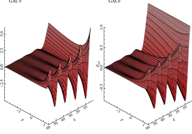
Figure 1: Generalised autocovariances and autocorrelations for the Gegenbauer process xt = (1−2νB+B2)−dξ
t, ξt∼WN(0, σ2) withd= 0.4, ν = 0.9, σ2= 1.
k
p γpk
GACV
10 20 30 40 50 60
−1 0
1
−2.5
0.0
2.5
5.0
k
p ρpk
GACF
10 20 30 40 50 60
−1 0
1
−0.5
0.0
0.5
1.0
p < 0.5/d, it converges at a faster rate than p = 1. Figure 1 illustrates the behavior of the GACV and GACF of a Gegenbauer process with ν = 0.9 and d = 0.4, for different values of
p < 1.25 and k = 1,2, . . . ,60. For p = −1/d, ρpk = 0, k = 3, . . . , as upt ha a non-invertible MA(2) representation.
5
Estimation
We shall consider a nonparametric estimator of the generalised autocovariance function based
on the periodogram of (x1, x,2, . . . , xn),
I(ωj) = 1 2πn
n
∑
t=1
(xt−x¯)e−ıωjt
2 ,
evaluated at the Fourier frequencies ωj = 2nπj ∈(0, π),1< j <[n/2].
defined as follows. Let M = [(n−1)/(2m)], then
ˆ
γpk = 1
M
M∑−1
j=0
Yj(p)cos(¯ωjk), (15)
where
Yj(p)=(2πI¯j)p
Γ(m) Γ(m+p) and
¯
Ij = m
∑
l=1
I(ωjm+l),
is the pooled periodogram over m non overlapping contiguous frequencies, whereas
¯
ωj =ωjm+(m+1)/2
are the mid range frequencies.
The estimator (15) is constructed based on the same principles of the variance profile es-timator considered by Luati, Proietti and Reale (2012), which is an extension of Hannan and Nicholls (1977) frequency domain estimator of the prediction error variance, which, in turn,
generalised the Davis and Jones (1968) estimator based on the raw periodogram. For simplicity of exposition, we have ruled out from estimation the frequencies 0 andπ, which require a special treatment, as the asymptotic theory based on the periodogram ordinates is slightly different in 0 and π. The latter can be included without substantially modifying the estimator, see the discussion in Hannan and Nicholls (1977).
The factor Γ(Γ(mm+)p) serves to correct for the asymptotic bias, E(Yj(p)) = (2πf(¯ωj))p, and pooling is required since the bias correction term exists only for p > −m, that for p = −1 requiresm >1. Furthermore, we shall prove that the asymptotic variance of the estimator (15) exists only forp >−m2. The underlying assumption is that the spectral density is constant over frequency intervals of length 2πmM . Notice that in the definition of ˆγpk the dependence on m is implicitly considered. The asymptotic properties of the estimator (15) are established by the following theorem.
Theorem 1 Let {xt}t∈T be the process xt =∑∞
j=0ψjξt−j where ξt ∼NID(0, σ2), ∑∞j=0|ψj|<
∞, ∑∞j=0|ψj||j|
1
2+δ <∞, δ >0, and with absolutely continuous spectral density function f(ω),
whose powersf(ω)p are integrable and uniformly bounded. Let us denote the vector of generalised
autocovariance functions up to lagKasγ′p = [γp0, γp1, . . . , γpK]′ and the corresponding estimator
with elements given by (15) as γˆ′p = [ˆγp0,γˆp1, . . . ,γˆpK]′. Then, γˆp →p γ and
√ n∗(γˆ
p−γp
)
where V={vkl;k, l= 0,1,2, . . . , K},with
vkl= 2 2π
∫ π
−π
[2πf(ω)]2pcos(ωk) cos(ωl)dω (17)
and n∗= m[C(mn;p,p)−1],with
C(m;p, q) = Γ(m+p+q)Γ(m)
Γ(m+p)Γ(m+q). (18)
The proof, given in Appendix A.1, is based on the asymptotic properties of the periodogram of a linear process, that require the strong convergence assumption on the coefficients of the
linear process, on the fractional moments of Gamma random variables and on a central limit theorem for non linear functionals of the periodogram due to Fa¨y, Moulines and Soulier (2002),
which can be applied when some regularity conditions on the functional of the spectrum and on the moments of the noise process are satisfied. The latter are easy to verify for a power function and a Gaussian process. Notice that the strong convergence condition on the filter coefficient
implies short-range dependence.
For m = 1 and p >0, Yj(p) is the inverse Laplace transform of [2πf(ωj)]−(p+1) evaluated at 2πI(ωj), that gives an estimator of [2πf(ωj)]p as in Taniguchi (1980), so that the consistency and the asymptotic normality of (15) follows from Taniguchi (1980). For largem, using Stirling’s approximation, Γ(m)/Γ(m+p)≈m−p,Y(p)
j ≈
(
2πI¯j)p, and interpreting ¯Ij as a kernel (Daniell) estimator of the spectral density at ¯ωj, theorem 6.1.2 in Taniguchi and Kakizawa (2000) can be applied, as the power transformation is a continuously twice differentiable function ofω and cos(kω) is even and continuous in [−π, π]. Since our result rests on the normality assumption, the additive component of asymptotic variance depending on the fourth cumulant vanishes.
Although our result is derived under more restrictive assumptions, it embodies a finite sample bias correction and establishes a lower bound form in the case of a negative p.
For m = 1 and p = 1 the estimator (15) gives the sample autocovariance at lag k, that is ˆ
γk = 1n∑tn=1−k(xt−x¯)(xt+k−x¯) fork= 0, . . . , n−1 and ˆγ−k= ˆγk, which follows from the relation
I(ωj) = 1 2π
∑
|h|<n ˆ
γhcos(ωjh).
prostapheresis formulae, equation (17) can be written as
vkl=
∞
∑
j=−∞
(γp,j+kγp,j+l+γp,j+kγp,j−l) (19)
which for m= 1 and p= 1 coincides with the asymptotic covariance of ˆγk.
In addition, the arguments of the proof allow us to derive the asymptotic covariance between
generalised autocovariance estimators across different power transformations, i.e.
Cov(ˆγpk,ˆγql) = 1
n(C(m;p, q)−1)
2m
2π
∫ π
−π
[2πf(ω)]p+qcos(ωk) cos(ωl)dω. (20)
A consistent estimator of (20) is
d
Cov(ˆγpk,ˆγql) = (C(m;p, q)−1) 1
M
M∑−1
j=1
(2πI¯j)p+qcos(¯ωjk) cos(¯ωjl)dω. (21)
Consistency follows from the same arguments that imply consistency of (15), see the last para-graph of the proof of theorem 1 in appendix A.1.
Under the assumptions of theorem 1, similar results can be derived for the generalised
auto-correlation function, that is estimated based on (15) by
ˆ
ρpk = ˆ
γpk ˆ
γp0
. (22)
Theorem 2 Let us consider the vectors ρ′
p = [ρp1, ρp2, . . . , ρpK]′ and ˆρp′ = [ˆρp1,ρˆp2, . . . ,ρˆpK]′ having components as in (3) and (22), respectively. Under the assumptions of theorem 1,
√ n∗(ρˆ
p−ρp
)
→dN(0,W) (23)
where W={wkl;k, l= 1,2, . . . , K}, with generic element given by the Bartlett’s formula
wkl=
∞
∑
j=−∞
(ρp,j+kρp,j+l+ρp,j+kρp,j−l+ 2ρp,kρp,lρ2p,j −ρp,kρp,jρp,j+l−ρp,lρp,jρp,j+k). (24)
The proof is in Appendix A.2 and it is a standard proof based on the same arguments that
lead to the proof of the Bartlett’s formula in the case whenp = 1. The asymptotic covariance matrix is estimated by replacing ˆρp for the population quantities into the expression forW.
In finite samples, the mean square errors of the GACV and GACF estimators, ˆγpk and ˆρpk, are a rather complicated function ofp,m, and the spectral properties ofxt. Luati, Proietti and Reale (2012) propose the use of the the jackknife (Quenouille, 1949, see Miller, 1974, and Efron
6
GACV-based Tests for White Noise
Two classes of tests for white noise can be based on the GACV. When applied to the residuals from a time series model, they serve as goodness of fit tests.
6.1 Generalised Portmanteau Tests
The generalised Portmanteau test statistic for lack of serial correlation, H0 :ρp1 =ρp2 =· · ·= ρpK = 0, is
BPp =n∗ K
∑
k=1
ˆ
ρ2pk. (25)
By Theorem 2, (25) provides an asymptotically χ2K test, generalising the Box-Pierce (1970) statistic BP =n∑Kk=1ρ˜2
kwhere ˜ρk=
∑n−k
t=1(xt−x¯)(xt+k−x¯)/∑nt=1(xt−x¯)2. The generalisation of the modified statistic LB =n(n+2)∑Kk=1(n−k)−1ρ˜2k, known as the Ljung-Box (1978) statistic, is also possible.
6.2 Generalised Milhøj Goodness of Fit Tests
A class of test statistics, generalising Milhøj (1981) goodness of fit test, exploits an important
property of the GACV, which is a direct consequence of Lemma 1: γ2p,0 = γp20 + 2
∑∞
j=1γpj2 . Hence, the ratio
Rp=
γ2p,0
γp20 = 1 + 2
∞
∑
j=1 ρ2pj
equals 1 for a WN process. A test of the null H0 :Rp = 1 against H1 : Rp > 1 can then be based on the estimated ratioRbp = ˆγγˆ2p,20
p0 , whose null distribution has variance
Var(Rbp) = 1
M {4C(m;p, p) +C(m; 2p,2p)−4C(m; 2p, p)−1}.
Hence, the test statistic
Mp =
b
Rp−1
√
Var(Rbp)
(26)
provides an asymptotically standard normal test.
The test (26) has the advantage of being independent of the choice of a particular truncation
lag K, and of depending of the full generalized autocorrelation function. For m = p = 1 it is coincident with the goodness of fit test of Milhøj (1981). It is related to the classes of
Hn = n∑Bj=1K2(j)˜ρ2j, where K(j) is a lag window, e.g. the Tukey-Hanning kernel K(j) = 0.5[1 + cos(πj/τ)], for |j|/τ ≤ 1, K(j) = 0, for |j|/τ > 1, and τ is the truncation parameter. The relationship has been made clear by Chen and Deo (2004a), see also Beran (1992), who propose a test based on Tn =
[
2π n
∑n−1
j=0f˜(ωj)
]−2 2π
n
∑n−1
j=0 f˜2(ωj), where ˜f(ωj) is an estimate
of the spectral density at the Fourier frequencyωj, and showed thatHn andn(πTn−0.5) have the same asymptotic distribution. Our test statistic depends on m and p. Their role will be illustrated by a Monte Carlo (MC) experiment. Notice that (26) withm >1 implies a Daniell-type estimation of the spectral density (the corresponding lag window is the sinc function; see
Priestley, 1981, p 440).
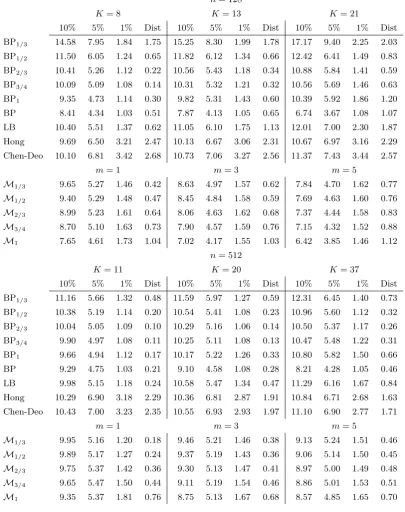
Table 1 reports the size of the WN tests proposed so far when xt ∼ NID(0,1), estimated by MC simulation using 50,000 replications, for three different significance levels (10%, 5%
and 1%), two sample sizes (128 and 512), using K autocorrelations (BPp tests and LB) or
τ =K truncation parameter (for the Hong and Chen-Deo statistics), and pooling parameterm. For BPp we report only the case m = 1. The column “Dist” provides the Euclidean distance between the upper tail quantiles of the MC distribution and those of the asymptotic distribution
(from 0.80 to 0.995 with step 0.005); hence, it measures the discrepancy between the empirical distribution and the asymptotic approximation in the upper 20% tail.
While it can be seen that the size properties of the BPp test are only marginally improved
by choosing p <1, as far as Mp is concerned, having p <1 yields more substantial gains. The heuristic explanation is that in finite sample fractional values of p have a normalisation effect on the distribution It should be recalled that the cube root transformation is the normalising transformation for a χ21 random variable. The Hong (1996) and Chen and Deo (2004a) tests suffer from size distortions, which are resolved in Chen and Deo (2004b) by taking a power
transformation of the test statistic, aiming at reducing the skewness of the distribution. In our case, the idea of transforming the periodogram is already embodied in GACV estimate. The
null distribution of theMp tests are displayed in figure 2, and compared to the Hong (1996) and Chen and Deo (2004a) tests, whose distribution before the correction is markedly right skewed.
Table 1: Effective sizes of WN tests. The data are generated asxt∼NID(0,1)
n= 128
K= 8 K= 13 K= 21
10% 5% 1% Dist 10% 5% 1% Dist 10% 5% 1% Dist BP1/3 14.58 7.95 1.84 1.75 15.25 8.30 1.99 1.78 17.17 9.40 2.25 2.03
BP1/2 11.50 6.05 1.24 0.65 11.82 6.12 1.34 0.66 12.42 6.41 1.49 0.83
BP2/3 10.41 5.26 1.12 0.22 10.56 5.43 1.18 0.34 10.88 5.84 1.41 0.59
BP3/4 10.09 5.09 1.08 0.14 10.31 5.32 1.21 0.32 10.56 5.69 1.46 0.63
BP1 9.35 4.73 1.14 0.30 9.82 5.31 1.43 0.60 10.39 5.92 1.86 1.20
BP 8.41 4.34 1.03 0.51 7.87 4.13 1.05 0.65 6.74 3.67 1.08 1.07 LB 10.40 5.51 1.37 0.62 11.05 6.10 1.75 1.13 12.01 7.00 2.30 1.87
Hong 9.69 6.50 3.21 2.47 10.13 6.67 3.06 2.31 10.67 6.97 3.16 2.29 Chen-Deo 10.10 6.81 3.42 2.68 10.73 7.06 3.27 2.56 11.37 7.43 3.44 2.57
m= 1 m= 3 m= 5
M1/3 9.65 5.27 1.46 0.42 8.63 4.97 1.57 0.62 7.84 4.70 1.62 0.77
M1/2 9.40 5.29 1.48 0.47 8.45 4.84 1.58 0.59 7.69 4.63 1.60 0.76
M2/3 8.99 5.23 1.61 0.64 8.06 4.63 1.62 0.68 7.37 4.44 1.58 0.83
M3/4 8.70 5.10 1.63 0.73 7.90 4.57 1.59 0.76 7.15 4.32 1.52 0.88
M1 7.65 4.61 1.73 1.04 7.02 4.17 1.55 1.03 6.42 3.85 1.46 1.12
n= 512
K= 11 K= 20 K= 37
10% 5% 1% Dist 10% 5% 1% Dist 10% 5% 1% Dist BP1/3 11.16 5.66 1.32 0.48 11.59 5.97 1.27 0.59 12.31 6.45 1.40 0.73
BP1/2 10.38 5.19 1.14 0.20 10.54 5.41 1.08 0.23 10.96 5.60 1.12 0.32
BP2/3 10.04 5.05 1.09 0.10 10.29 5.16 1.06 0.14 10.50 5.37 1.17 0.26
BP3/4 9.90 4.97 1.08 0.11 10.25 5.11 1.08 0.13 10.47 5.48 1.22 0.31
BP1 9.66 4.94 1.12 0.17 10.17 5.22 1.26 0.33 10.80 5.82 1.50 0.66
BP 9.29 4.75 1.03 0.21 9.10 4.58 1.08 0.28 8.21 4.28 1.05 0.46 LB 9.98 5.15 1.18 0.24 10.58 5.47 1.34 0.47 11.29 6.16 1.67 0.84 Hong 10.29 6.90 3.18 2.29 10.36 6.81 2.87 1.91 10.84 6.71 2.68 1.63
Chen-Deo 10.43 7.00 3.23 2.35 10.55 6.93 2.93 1.97 11.10 6.90 2.77 1.71
m= 1 m= 3 m= 5
M1/3 9.95 5.16 1.20 0.18 9.46 5.21 1.46 0.38 9.13 5.24 1.51 0.46
M1/2 9.89 5.17 1.27 0.24 9.37 5.19 1.43 0.36 9.06 5.14 1.50 0.45
M2/3 9.75 5.37 1.42 0.36 9.30 5.13 1.47 0.41 8.97 5.00 1.49 0.48
M3/4 9.65 5.47 1.50 0.44 9.11 5.19 1.54 0.46 8.86 5.01 1.53 0.51
[image:16.595.98.504.166.679.2]Figure 2: Distribution of white noise tests statistics based on 50,000 simulations of Gaussian
xt∼NID(0,1) withn= 128, m= 1, K = 8.
−3 −2 −1 0 1 2 3 4 5 6 7 8 9 10 11
0.1 0.2 0.3 0.4 0.5
M1 M3/4 M2/3 M1/2 M1/3
Hong Chen−Deo
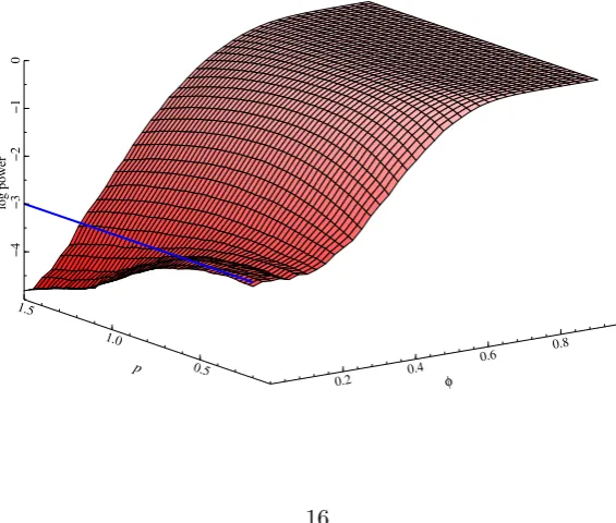
Figure 3: Logarithm of the power function of the testMp based on 20,000 simulations from the AR(1) process xt=φxt−1+ξt, ξt ∼NID(0,1) with n= 128, m= 1. The straight line is drawn at the log-size ln(0.05).
log power
φ p
0.2 0.4
0.6 0.8
0.5 1.0
1.5
−4
−3
−2
−1
[image:17.595.153.436.490.730.2]Figure 4: US Gross domestic product: quarterly growth rates (1947.2-2012.1), periodogram and GACF, estimated withm= 3.
1950 1960 1970 1980 1990 2000 2010
−2 0 2
4 Quarterly growth rates
k p
ρpk
Generalised autocorrelation function
1 2 3 4 5 6 7 8 9 10 11 12 13 14 15
0
2
−0.5
0
0.5
1
7
Feature matching: a Yule-Walker spectral estimator based on
the GACV
An important use of the GACV is in extracting features of interest from a time series. Figure
4 displays the quarterly growth rate of the US Gross Domestic Product (1947.2-2012.1), along with its estimated GACF, usingm= 3 forpranging from -1 to 3 (recall thatm≥3 is needed to estimate the GACV atp=−1 with finite asymptotic variance). The cyclical nature of this series has represented a long debated issue. See Harvey and J¨ager (1997) and the references therein.
The periodogram (see also figure 5) does indeed display large ordinates at low frequencies and ˆ
ρpk describes a pseudo-cyclical pattern for values of p greater than 1. However, parsimonious ARMA models, selected on the basis of information criteria, fail to capture the cyclical feature
of GDP growth and fit a monotonically decreasing spectrum with a global maximum at the origin.
In this section we propose a Yule-Walker spectral estimator based on the GACV. We illustrate that allowing for a power transformation parameter greater than 1 amounts to boosting the
The Yule-Walker estimation method is very popular in time series estimating the
autoregres-sive parameters (see Percival and Walden, 1993, for a review). Recently, Xia and Tong (2011) have introduced an approach for time series modelling, aiming at matching stylised features of the time series, such as the autocorrelation structure. We consider here a feature matching
Yule-Walker estimate of the spectrum with a similar intent, which uses the GACV at different values ofp.
LetΓp,Kdenote the Toeplitz matrix, formed from the GACV, with generic elementγp,|h−k|, h, k=
0, . . . , K−1, let γp,K = (γp1, . . . , γpK)′, and φp,K = (φ1p, . . . , φpK)′. The latter is a K×1 vec-tor of AR coefficients satisfying the Yule-Walker equations Γp,Kφ
p,K = γp,K. The polynomial
φp(B) = 1−φ1pB− · · ·φpKBK, characterises the AR approximation of the processupt, and pro-vides directly the spectral factorisation [2πf(ω)]p ∝[φ
p(e−ıω)φp(eıω)]−1. By (9) we can obtain the AR approximation of orderK′> K for the original process,π(B)xt=ξt,π(B) = [φp(B)]1/p, or, equivalently, the moving average representation xt = ψ(B)ξt, ψ(B) = [φp(B)]−1/p. Given a time series realisation, we replace the theoretical GACF with the estimated one to get
ˆ
φp,K = ˆΓ−1
p,Kγˆp,K, applying (9), we obtain different estimates for the spectrum of the time series according to the value of p, ˆfp(ω).
Figure 5 displays the periodogram of the US GDP quarterly growth rate series and the spectral estimates corresponding to p= 0.5,1,2,3,4, using K = 3 sample GACVs. No cyclical peaks is identified for p≤1, but as p increases, the cyclical properties of GDP growth become prominent. For judging which spectral estimate is more suitable, we consider a measure of
deviance equal to minus twice the Whittle’s likelihood (Whittle, 1961), as advocated by Xia and Tong (2011), dev(p) = ∑nj=1[I(ωj)
ˆ
fp(ωj) + ln ˆfp(ωj)
]
. The plot of dev(p) versus p (right panel of figure 5) suggests the value ˜p= 2.65.
The spectral peak, corresponding to a period of roughly 2.5 years (10 quarters), can alterna-tively be identified by increasing the AR order, as figure 6 shows, but there is a risk of overfitting
the sample spectrum in other frequency ranges.
8
Time Series Cluster and Discriminant Analysis
Figure 5: US Gross domestic product (1947.2-2012.1): spectrum estimation by thep-Yule-Walker method usingK = 3.
p=0.5 × ω p=2 × ω p=4 × ω
p=1 × ω p=3 × ω
0.0 0.5 1.0 1.5 2.0 2.5 3.0
0.1 0.2 0.3 0.4 0.5 0.6 0.7 0.8
0.9 Periodogram and spectrum
ω
p=0.5 × ω p=2 × ω p=4 × ω
p=1 × ω p=3 × ω
0.5 1 1.5 2 2.5 3 3.5 4
−132.8 −132.6 −132.4 −132.2 −132.0 −131.8 Deviance
p
Figure 6: US Gross domestic product (1947.2-2012.1): Yule-Walker estimates of the spectrum (as a function of p andω), based on different GACV orders.
ω p
f
(
ω
)
K=3
1
2
3 1
2 3
4
0.25
0.50
0.75
ω p
f
(
ω
)
K=7
1
2
3 1
2 3
4
0.25
0.50
0.75
ω p
f
(
ω
)
K=11
1
2
3 1
2 3
4
0.25
0.50
[image:20.595.110.481.434.741.2]equivalent to the Euclidean distance between the GACVsγi,pk and γj,pk of the two processes:
d2ij,p = 21π∫−ππ{[2πfi(ω)]p−[2πfj(ω)]p}2dω = ∑∞k=−∞(γi,pk−γj,pk)2
= γi,2p,0+γj,2p,0−2∑∞k=−∞γi,pkγj,pk.
(27)
Thep-sd (27) encompasses the Euclidean distance (p= 1), referred to as the quadratic distance in Hong (1996) and the Hellinger distance (p = 1/2). It can also be based on the normalised spectral densities of the two processes, in which case the autocorrelationsρpk replace the auto-covariances in (27).
The p-sd can be estimated by
ˆ
d2ij,p = (ˆγi,p0−γˆj,p0)2+ 2
K
∑
k=1
(ˆγi,pk−ˆγj,pk)2.
or, if the autocorrelations are used,
ˆ
d2ij,p = 2 K
∑
k=1
(ˆρi,pk−ρˆj,pk)2.
The p-sd can be used for clustering time series and estimation by feature matching, if the distance is computed with respect to the theoretical GACF implied by a time series model. In the stationary case, for which |ρ1k|declines at a geometric or hyperbolic rate, when p is larger than 1, the contribution of low order, high autocorrelations to the overall distance will be higher. On the contrary, for values of 0< p < 1 less than unity, the contribution of high order, small autocorrelations, will be comparatively larger. Similar considerations hold for negative p, but with reference to the inverse autocorrelations.
Another use is in discriminant analysis. The relevance of generalising the distance to
frac-tional and negative values of p is illustrated by an application of Fisher’s linear discriminant analysis (Mardia, Kent and Bibby, 1979) to a simulated data set.
N = 1,050 time series of sizenwere generated under three different models: N1 = 600 AR(1) series with coefficient φ randomly drawn from a uniform distribution in [0.1, 0.9], N2 = 300
MA(1) series with coefficient θ uniformly distributed in [−0.9,−0.1], and N3 = 150 fractional noise series with memory parameter uniformly distributed in [0.1, 0.4].
Two-thirds of the series were used as a training sample to estimate the canonical variates,
For the training sample the two canonical variates are obtained from the generalised
eigen-vectors of the between groups deviance matrix, B, satisfyingBa=λa, a′Wa= 1, whereW is
the within groups deviance matrix and λis the generalised eigenvalue ofB, forλ >0.
The test series are then classified according to the smallest Mahalanobis’ distance to the
GACF group means, which amounts to computing the canonical scores for the test series, by combining linearly the GACFs using the weights a computed on the training sample, and
as-signing the series to the group for which the distance with the canonical means is a minimum. Different values ofpyield different discriminant functions and different results. We select the optimal solution (across the values ofp) as the one minimising the missclassification rate (MR) computed for the test sample.
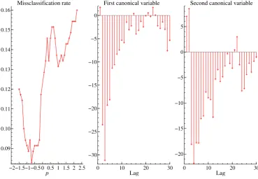
Figure 7 displays the MRs for values of p in the range [-2, 2] for a simulation dataset with
n = 1,000, K = 30. For estimating the GACF we set m = 6. The value of p yielding the smallest MR resulted ˜p = −0.7 (replicating the experiment, we always obtain values in the range [-1,-0.2]); the improvement with respect to p= 1 is large (around a 5% reduction in the MR). The generalised eigenvectors a, defining the two canonical variates for ˜p are also plotted.
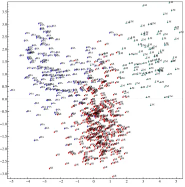
Interestingly, the first canonical variable assigns declining (negative) weights to the GACF from 2 toK, whereas the second is a contrast between the first two GACF and the higher order ones. The two canonical variate scores for the training sample are displayed in figure 8: it illustrates
that the solution provides an effective separation of the three groups.
9
Conclusions
The paper has defined the generalised autocovariance function and has shown its potential for three different analytic tasks: testing for white noise, the estimation of the spectrum of cyclical
time series, and time series methods based on the distance between stochastic processes, like cluster and discriminant analysis.
By tuning the power transformation parameter given features of a time series can be em-phasised or muted for a particular purpose. In this respect, we think that the proposed feature
matching Yule-Walker spectral estimator based the GACV has very good potential for the iden-tification of spectral peaks of time series affected by noise. Aspincreases, the contribution of the noise to the spectrum will be subdued to some extent and the AR fit will attempt at matching
the cyclical properties of the series more closely.
Figure 7: Canonical analysis of simulated series: missclassification rate as a function of p, and canonical variates weights for the optimal p.
−2−1.5−1−0.5 0 0.5 1 1.5 2 2.5 0.09
0.10 0.11 0.12 0.13 0.14 0.15 0.16
Missclassification rate
p 0 10 20 30
−30 −25 −20 −15 −10 −5 0
Lag First canonical variable
0 10 20 30 −20
−15 −10 −5 0 5
Lag
Figure 8: Canonical analysis of simulated series: plot of the two canonical variates for the
training sample, consisting of 400 AR series, 200 MA series and 50 fractional noise series. The value of p is -0.7.
−5 −4 −3 −2 −1 0 1 2 3 4 5
−3.0 −2.5 −2.0 −1.5 −1.0 −0.5 0.0 0.5 1.0 1.5 2.0 2.5 3.0 3.5 AR AR AR AR AR AR AR AR AR AR AR AR AR AR AR AR AR AR AR AR AR AR AR AR AR AR AR AR AR AR AR AR AR AR AR AR AR AR AR ARAR AR AR AR AR AR AR AR AR AR AR AR AR AR AR AR AR AR AR AR AR AR AR AR AR AR AR AR AR AR AR AR AR AR AR AR AR AR AR AR AR AR AR AR AR AR AR AR AR AR AR AR AR AR AR AR AR AR AR AR AR AR AR AR AR AR AR AR AR AR AR AR AR AR AR AR AR AR AR AR AR AR AR AR AR AR AR AR AR AR AR AR AR AR AR AR AR AR AR AR AR AR AR AR AR AR AR AR AR AR AR AR AR AR AR AR AR AR AR AR AR AR AR AR AR AR AR AR AR AR AR AR AR AR AR AR AR AR AR AR AR AR AR AR AR AR AR AR AR AR AR AR AR AR AR AR AR AR AR AR AR AR AR AR AR AR AR AR AR AR AR AR AR AR AR AR AR AR AR AR AR AR AR AR AR AR AR AR AR AR AR AR AR AR AR AR AR AR AR AR AR AR AR AR AR AR AR AR AR AR AR AR AR AR AR AR AR AR AR AR AR AR AR AR AR AR AR AR AR ARAR AR AR AR AR AR AR AR AR AR AR AR AR AR AR AR AR AR AR AR AR AR AR AR AR AR AR AR AR AR AR AR AR AR AR AR AR ARAR AR AR AR AR AR AR AR AR AR AR AR AR AR AR AR AR AR AR AR AR AR AR AR AR AR AR AR AR AR AR AR AR AR AR AR AR AR AR AR AR AR AR AR AR AR AR AR AR AR AR AR AR AR AR AR AR AR AR AR AR AR AR AR AR AR AR AR AR AR AR AR AR AR AR AR AR AR AR AR AR AR AR AR AR AR AR AR AR AR AR AR MA MA MA MA MA MA MA MA MA MA MA MA MA MA MA MA MA MA MA MA MA MA MA MA MA MA MA MA MA MA MA MA MA MA MA MA MA MA MA MA MA MA MA MA MA MA MA MA MA MA MA MA MA MA MA MA MA MA MA MA MA MA MA MA MA MA MA MA MA MA MA MA MA MA MA MA MA MA MA MA MA MA MA MA MA MA MA MA MA MA MA MA MA MA MA MA MA MA MA MA MA MA MA MA MA MA MA MA MA MA MA MA MA MA MA MA MA MA MA MA MA MA MA MA MA MA MA MA MA MA MA MA MA MA MA MA MA MA MA MA MA MA MA MA MA MA MA MA MA MA MA MA MA MA MA MA MA MA MA MA MA MA MA MA MA MA MA MA MA MA MA MA MA MA MA MA MA MA MA MA MA MA MA MA MA MA MA MA MA MA MA MA MA MA MA MA MA MA MA MA LM LM LM LM LM LM LM LM LM
spectrum or autocorrelation function. We leave to future research the generalisation of Bartlett’s
tests (Bartlett, 1954) for white noise based on the normalized integrated power transformation of the spectrum (see Priestley, sec. 6.2.6., Durlauf, 1991, Deo, 2000, and Delgado, Hidalgo and Velasco, 2005).
Another extension that we have not investigated is the partial generalised autocorrelation function, which can be used as an additional model identification tool, complementing the
tra-ditional one. El Ghini and Francq (2006) advocated the use of the inverse partial ACF, and their results encourage further investigating this direction.
A
Appendix
A.1 Proof of theorem 1
Let us consider the estimator (15). Under the assumption ∑∞j=0|j|12|ψ
j|<∞, the periodogram ordinates of a linear process with finite fourth moment evaluated at the Fourier frequencies 0 < ω1 < · · · < ωk < π are asymptotically IID exponentials with means equal to f(ωj),
j = 1,2, . . . , k (Brockwell and Davis, 1991, Theorem 10.3.2). If M and m are large enough for asymptotics and Mm is small enough for f(ω) to be constant over frequency intervals of length 2Mπm, then, for fixed m, ¯Ij can be interpreted as a Daniell type estimator for f(¯ωj) and 2πI¯j ∼ 2πf(¯ωj)Gm, where the Gm are independent and identically distributed basic Gamma random variables with shape parameter equal tom (see Koopmans, 1974, pp. 269-270). Hence, E(Yj(p)) = (2πf(¯ωj))p and Cov(Yj(p), Y
(q)
j ) = (C(m;p, q)−1)[2πf(¯ωj)]p+q.Notice that, forp=q, Var(Yj(p)) exists forp >−m2.
Let us consider the sequence
Sn(Yj(p)) = M∑−1
j=0 bj
{
Yj(p)−(2πf(¯ωjk))p
}
(28)
where bj =cj/(s(c2j))
1
2, with c
j = cos(¯ωjk) and s(c2j) =
∑M−1
j=0 cos2(¯ωjk). By construction, the coefficients bj satisfy ∑Mj=0−1b2j = 1 and max0≤j≤M−1|bj| → 0, since cos(ωk) is a function of bounded variation for ω∈(−π, π).
If theYj(p)were IID or, equivalently, if the process{xt}t∈T were a Gaussian white noise, then a central limit theorem for linear combinations of independent random variables would directly apply to Sn(Yj(p)), as in Luati, Proietti and Reale (2012). Given that the random variables
Yj(p) are asymptotically independent, an intermediate step is needed, that consists in proving the asymptotic negligibility of the term Sn(Yj(p))−Sn(Zj(p)), where Z
(p)
j = (2πI¯j,ξ)pΓ(Γ(mm+)p), ¯Ij,ξ denoting the pooled periodogram of (ξ1, . . . , ξn) at ¯ωj. In this way, a central limit theorem for Sn(Yj(p)) can be proved as a consequence of a central limit theorem for Sn(Zj(p)), see Fa¨y, Moulines and Soulier (2002). A similar approach is in Kl¨upperberg and Mikosch (1996), though
in a slightly different context. The implications of Sn(Yj(p))−Sn(Zj(p))→p 0 on a central limit theorem forSn(Yj(p)) are proved based on a Bartlett-type decomposition that relates the pooled periodogram of the observed variables with the pooled (pseudo) periodogram of the noise process
and requires the strong assumption on the filter coefficients, ∑∞j=0|ψj||j|
1
2+δ <∞,δ <0. The
latter condition implies short-range dependence on the process. Some additional regularity
to prove the weak convergence of Sn(Yj(p)) to Sn(Zj(p)). In our context, Theorem 1 of Fa¨y, Moulines and Soulier (2002) applies toSn(Yj(p)), since assumptions 1, 2, 4, 7 and S1, that have to be satisfied when the noise term is Gaussian, hold. Specifically, assumptions 1 and 2 concern
the coefficients bj, assumption 4 requires the existence of the asymptotic variance ofSn(Yj(p)), which occurs for p > −m2, assumption 7 is the convergence on the filter coefficients necessary for the Bartlett decomposition and assumption S1, such that maxx∈R|φ(x)|+|φ
′(x)|+|φ′′(x)|
1+|x|ν <∞,
is satisfied forφ(x) =xp and for a Gaussian process, having all finite moments µ≥min{8ν,4}. Hence,
Sn(Yj(p))→dN
0,
M∑−1
j=0
b2jVar(Yj(p))
.
As a function of the estimator (15), by multiplying (28) by M1 (s(c2j))12 and rearranging,
1
M
M∑−1
j=0
cjYj(p) →dN
1
M
M∑−1
j=0
cj(2πf(¯ωj))p, 1
M
M∑−1
j=0
c2j(2πf(¯ωj))2p 1
M(C(m;p, p)−1)
.
(29) By taking the limits (see also Theorem 2 of Fa¨y, Moulines and Soulier, 2002)
√ n∗(ˆγ
pk−γpk)→dN (0, vkk), (30)
wherevkk= 22π
∫π
−π(2πf(ω))2pcos2(ωk)dω,n∗=n(m(C(m;p, p)−1))−1 and C(m;p, q) is as in (18). It is straightforward to get the covariance between ˆγpk and ˆγpl asvkl as in (17). Taking
vkl for k = 0,1, . . . , K and setting the results in matrix notation complete the proof of the asymptotic distribution of the generalised autocovariance estimator.
Consistency of ˆγpk follows by the Chebychev weak law of large numbers, applied to the sequence of random variables in (29) and from the convergence of the Riemannian sum to the integral. This completes the proof of theorem 1.
A.2 Proof of theorem 2
The asymptotic joint normality of the generalised autocorrelation estimators is obtained by applying the delta method to the transformation operated by the function g : RK+1 → RK
which associates the vector ˆρp, having components ˆρpj = γγˆˆpjp0, j = 1, . . . , K, with the vector
ˆ
γpj,j = 0,1, . . . , K, with components as in (15). The covariance matrix of ˆρp is W = DVD′
with partial derivatives matrix D = 1
γp0
[
−ρp IK], so that the generic element of W is (as in
Brockwell and Davis, 1991, proof of theorem 7.2.1) wkl =vkl−ρpkv0l−ρplvk0+ρpkρplv00.By
References
[1] Bartlett, M. S. (1954). Problemes de l’analyse spectral des series temporelles stationnaires. Publ. Inst. Statist. Univ. Paris, III–3 119–134.
[2] Battaglia, F. (1983), Inverse Autocovariances and a Measure of Linear Determinism For a Stationary Process,Journal of Time Series Analysis, 4, 7987 .
[3] Battaglia, F. (1988), On the Estimation of the Inverse Correlation Function,Journal of Time Series Analysis, 9, 1-10.
[4] Battaglia, F., Bhansali, R. (1987), Estimation of the Interpolation Error Variance and an Index of Linear Determinism,Biometrika, 74, 4, 771–779.
[5] Beran, J. (1992), A Goodness-of-Fit Test for Time Series with Long Range Dependence,
Journal of the Royal Statistical Society, Series B, 54, 3, 749–760.
[6] Bhansali, R. (1993), Estimation of the Prediction Error Variance and an R2 Measure by
Autoregressive Model Fitting, Journal of Time Series Analysis, 14, 2, 125–146.
[7] Box, G.E.P., and Cox, D.R. (1964), An analysis of transformations (with discussion),Journal
of the Royal Statistical Society, B, 26, 211–246.
[8] Box, G. E. P., and Pierce, D. A. (1970), Distribution of Residual Autocorrelations in
Autoregressive-Integrated Moving Average Time Series Models,Journal of the American Sta-tistical Association, 65, 1509-1526.
[9] Brockwell, P.J. and Davis, R.A. (1991), Time Series: Theory and Methods, Springer-Verlag, New York.
[10] Chen, W.W. and Deo, R.S. (2004a), A Generalized Portmanteau Goodness-of-Fit Test for Time Series Models, Econometric Theory, 20, 382–416.
[11] Chen, W.W. and Deo, R.S. (2004b), Power transformations to induce normality and their
applications. Journal of the Royal Statistical Society,Series B, 66, 117-130.
[12] Cleveland, W.S. (1972), The Inverse Autocorrelations of a Time Series and Their
Applica-tions, Technometrics, 14, 2, 277–293.
[13] Davis, H.T. and Jones, R.H. (1968), Estimation of the Innovation Variance of a Stationary
[14] Delgado, M.A., Hidalgo, J. and Velasco, C. (2005), Distribution Free Goodness-of-Fit Tests
for Linear Processes, Annals of Statistics, 33, 2568–2609.
[15] Deo, R.S. (2000), Spectral Tests of the Martingale Hypothesis under Conditional
Het-eroscedasticity, Journal of Econometrics, 99, 291-315.
[16] Doob, J.L. (1953), Stochastic Processes, John Wiley and Sons, New York.
[17] Durlauf, S.N. (1991). Spectral Based Testing of the Martingale Hypothesis, Journal of Econometrics, 50, 355–376.
[18] Efron, B., and Tibshirani R.J. (1993),An Introduction to the Bootstrap, Chapman&Hall.
[19] El Ghini, A., and Francq, C. (2006), Asymptotic Relative Efficiency of Goodness-Of-Fit Tests Based on Inverse and Ordinary Autocorrelations, Journal of Time Series Analysis, 27,
843–855.
[20] Erd´elyi A., Magnus W., Oberhettinger F., and Tricomi F.G. (1953),Higher Transcendental Functions, vol. II, Bateman Manuscript Project, McGraw and Hill.
[21] Fa¨y, G., Moulines, E. and Soulier, P. (2002), Nonlinear Functionals of the Periodogram, Journal of Time Series Analysis, 23, 523–551.
[22] Fuller, W.A. (1996), Introduction to Statistical Time Series, John Wiley & Sons.
[23] Gould, H.W. (1974), Coefficient Identities for Powers of Taylor and Dirichlet Series, The American Mathematical Monthly, 81, 1, 3–14.
[24] Gradshteyn I.S. and Ryzhik I.M. (1994)Table of Integrals, Series, and Products Jeffrey A.
and Zwillinger D. Editors, Fifth edition, Academic Press.
[25] Graham, R.L., Knuth, D.E. and Patashnik, O., (1994), Concrete Mathematics, Addison-Wesley Publishing Company.
[26] Gray, H. L., Zhang, N.-F. and Woodward, W. A. (1989), On Generalized Fractional Pro-cesses. Journal of Time Series Analysis, 10, 233-257.
[27] Hannan, E.J. and Nicholls, D.F. (1977), The Estimation of the Prediction Error Variance,
[28] Harvey, A.C., and J¨ager, A. (1993), Detrending, Stylized Facts and the Business Cycle,
Journal of Applied Econometrics, 8, 231–247.
[29] Hong, Y. (1996), Consistent Testing for Serial Correlation of Unknown Form,Econometrica, 64, 4 837–864.
[30] Kl¨upperberg, C., Mikosch, T. (1996), Gaussian Limit Fields for the Integrated Periodogram,
The Annals of Probability, 6, 3 969–991.
[31] Koopmans, L.H. (1974),The Spectral Analysis of Time Series, Academic Press.
[32] Ljung, G. M. and Box, G. E. P. (1978), On a Measure of Lack of Fit in Time Series Models, Biometrika, 65, 297-303.
[33] Luati, A., Proietti, T. and Reale, M. (2012), The Variance Profile,Journal of the American
Statistical Association, 107, 498, 607–621.
[34] Mardia, K., Kent, J. and Bibby, J. (1979). Multivariate Analysis, Academic Press.
[35] Milhøj, A. (1981), A Test of Fit in Time Series Models,Biometrika, 68, 1, 167–177.
[36] Miller, R.G. (1974), The Jackknife–A Review. Biometrika, 61, 1, 1–15.
[37] Percival, D.B. and Walden, A.T. (1993),Spectral Analysis for Physical Applications, Cam-bridge University Press.
[38] Pourahmadi, M. (2001),Foundations of Time Series Analysis and Prediction Theory, John
Wiley and Sons.
[39] Priestley, M.B. (1981),Spectral Analysis and Time Series, John Wiley and Sons.
[40] Quenouille, M.H. (1949), Approximate Tests of Correlation in Time Series. Journal of the Royal Statistical Society, Series B, 11, 68-84.
[41] Taniguchi, M. (1980), On Estimation of the Integrals of Certain Functions of Spectral
Density,Journal of Applied Probability, 17, 1, 73–83.
[42] Taniguchi, M. and Kakizawa, Y. (2000), Asymptotic Theory for Statistical Inference of Time Series, Springer.
[43] Tieslau, M.A., Schmidt, P. and Baillie, R.T. (1996), A Minimum Distance Estimator for
[44] Tukey, J. W. (1957), On the comparative anatomy of transformations, Annals of
Mathe-matical Statistics, 28, 602–632.
[45] Walden, A. T. (1994), Interpretation of Geophysical Borehole Data via Interpolation of
Fractionally Differenced White-Noise, Journal of the Royal Statistical Society, Series C, 43, 335–345.
[46] Whittle, P. (1961), Gaussian estimation in stationary time series, Bulletin of the
Interna-tional Statistical Institute, 39, 105–129.
[47] Woodward, W. A., Cheng, Q. C. and Gray, H. L. (1998), Ak-Factor GARMA Long-memory Model. Journal of Time Series Analysis, 19, 485-504.