A win win monetary policy in Canada

Munich Personal RePEc Archive

A win-win monetary policy in Canada

Kitov, Oleg and Kitov, Ivan

IDG RAS, University of Oxford, Department of Economics

30 March 2011

A win-win monetary policy in Canada

Oleg Kitov, Department of Economics, University of Oxford

Ivan Kitov, Institute for the Geospheres’ Dynamics, RAS

Abstract

The Lucas critique has exposed the problem of the trade-off between changes in monetary policy and structural breaks in economic time series. The search for and characterisation of such breaks has been a major econometric task ever since. We have developed an integral technique similar to CUSUM using an empirical model quantitatively linking the rate of inflation and unemployment to the change in the level of labour force in Canada. Inherently, our model belongs to the class of Phillips curve models, and the link between the involved variables is a linear one with all coefficients of individual and generalized models obtained by empirical calibration. To achieve the best LSQ fit between measured and predicted time series cumulative curves are used as a simplified version of the 1-D boundary elements (integral) method. The distance between the cumulative curves (in L2 metrics) is very sensitive to structural breaks since it accumulates true differences and suppresses uncorrelated noise and systematic errors. Our previous model of inflation and unemployment in Canada is enhanced by the introduction of structural breaks and is validated by new data in the past and future. The most exiting finding is that the introduction of inflation targeting as a new monetary policy in 1991 resulted in a structural break manifested in a lowered rate of price inflation accompanied by a substantial fall in the rate of unemployment. Therefore, the new monetary policy in Canada is a win-win one.

Key words: structural break, inflation, unemployment, labour force, modelling, Canada JEL classification: E3, E6, J21

Introduction

The Bank of Canada was one of the first worldwide to announce the policy of inflation targeting

between 1 and 3 percentage points per year (Bank of Canada 2010). This objective was

originally articulated in 1988 and this new monetary policy was formally introduced in 1991.

The goal to retain the level of price inflation in the designated range may introduce a

measurable disturbance in a given economy and affect the links between major macroeconomic

variables, as was explicitly indicated by Lucas (1976). Then, the basis of price inflation

targeting might be corrupted since inflation sensitivity to other macroeconomic variables may

change. In this case, one would have observed “structural breaks” in the relationships between

such macroeconomic time series as inflation and unemployment (or some other measures of

economic activity), i.e. sudden changes in the related empirically derived coefficients (Hostland

1995).

In this paper, we quantitatively estimate and statistically characterize the evolution of

several deterministic relationships between inflation and unemployment in Canada. One of our

major objectives is to reveal and better estimate in time and amplitude the structural break

potentially associated with the introduction of inflation targeting. For this purpose, we have

adapted from physics and engineering the method of boundary elements in its simplified form

of cumulative curves, which is complementary to the econometric techniques based on dynamic

regression damaging the estimation of actual links between time series (Chiarella and Gao

2002).

Having estimated with the 1D boundary elements method a number of statistically reliable

deterministic models of inflation and unemployment (Kitov and Kitov 2010) we are able to find

the trade-off between these variables, which may be best expressed in cumulative values

(integrals). Page (1954) introduced a technique for univariate time series, which comprises the

statistical basis for our empirical approach. This is a well-known CUSUM (cumulative sum)

control chart. We use essentially bivariate and trivariate deterministic model with nonstationary

time series and have to calibrate the model together with testing for structural breaks. Therefore,

it is instructive to plot both (measured and predicted) times series instead of their demeaned

difference. However, all statistical inferences related to the CUSUM method can be applied

one-to-one to the model residual.

Any structural break is (by definition) accompanied by the change in relevant model

coefficients. When both sides of a given bivariate relationship are integrated over time the

structural break must manifest itself in the divergence of integrals starting from the break point.

Statistically, this approach is potentially a more reliable one than those based on specific

features of dynamic time series. Firstly, all uncorrelated noise is suppressed by destructive

interference. Secondly, any amplitude dependent systematic error is compensated by a

proportional shift in the slope and all amplitude independent systematic errors add up to the free

term. It is worth noting that nobody is able to measure true values of such macroeconomic

variables as inflation and unemployment; they both depend on definitions which are never

perfect. Hence, one always has systematic errors in these time series, which are not easy to

handle in the dynamic representation since they may introduce an amplitude-dependent bias.

Thirdly, the effect of the change in coefficients is steadily amplified (accumulated) by

constructive interference with increasing signal to noise ratio. This effect is crucial for statistical

inferences. Literally, the integral curves representing both sides of the equation diverge at a

constant rate after the year of structural break.

For our model, all three benefits are working together. An additional (but not uncommon

for econometrics) benefit consists in the fact that the cumulative sums of price inflation and the

change rate of labour force are represented by actually measured overall price and labour force.

Since the accuracy of price and labour force measurements is relatively high and approximately

time independent the cumulative error terms in the time series of inflation and the change rate

of labour force must always add up to the level of the measurement accuracy, i.e.

standard statistical inferences. In reality, all past values of labour force and prices are routinely

revised with every new measurement to match the newly measured value.

However, all these benefits are conditional on the presence of a deterministic link. When a

purely statistical link between two stochastic variables is integrated, the uncorrelated error term

creates a stochastic trend, the systematic error correlates with the stochastic trend and cannot be

separated from it, and the divergence between the integral curves after the break is not a

quasi-linear one. This is the reason why econometricians do not use CUSUM. There is a slight

prejudice against deterministic links in econometrics.

Fortunately, a variety of actual measurements reported by developed countries allow

distinguishing between deterministic and stochastic links (Kitov 2007a; Kitov and Kitov 2010).

It was found and proved by strict and extensive statistical and econometric tests (Kitov, Kitov,

and Dolinskaya 2007) that the evolution of price inflation and the rate of unemployment is

driven by the change in the level of labour force. For Canada, we estimated these links several

years ago (Kitov 2007b), without structural breaks however. Thus, we can validate the previous

models using new data and refine them allowing for structural breaks.

Several years ago we introduced a concept linking by linear and lagged relationships price

inflation and unemployment in developed countries to the change rate of labour force (Kitov,

2006). Corresponding model is a completely deterministic one with the change in labour force

being the only driving force causing all variations in the pair unemployment/inflation. Since

2006, many empirically estimated models have been tested econometrically (conditional on the

length of time series) and the presence of cointegrating relations has been demonstrated.

Formally, our model is a somewhat degenerate version and a marginal extension of such

economic/econometric models as the conventional Phillips curve or the new Keynesian Phillips

curve. For example, among the diversity of economic/financial variables used by Stock and

Watson (2003, 2008) as predictors of inflation, the set included approximately 200 time series,

the change in labour force was absent. Thus, it was instructive to extend this set with labour

force and to conduct a similar statistical investigation.

We have revealed for many developed countries (the USA, Japan, France and Germany

among others) that, in purely econometric terms, this rather countable than measurable

macroeconomic predictor is characterized by an extraordinary (relative to other tested

parameters) power and inflation is not “hard to forecast”, as concluded by Stock and Watson

(2007). The change in labour force in the biggest developed economies is so good a predictor

that there is no need to use autoregressive properties of inflation and other variables. In this

errors not to stochastic properties of the involved processes.

Here we have to notice that such an extensive usage of autocorrelation in the modelled

time series implies that the researcher does not expect any other macroeconomic variables to be

involved. Mathematically, it is a flawed way of quantitative analysis – autocorrelation terms

severely mask any real driving force since the modelled time series is decomposed into a set of

non-orthogonal functions (variables). The long history of econometric research has

unambiguously demonstrated that the AR and similar statistical models are able to describe

observations only superficially and suppress the signals from actual sources of inflation. Even

with wrong predictors, the Phillips curve approach works best when inflation changes very fast

and autocorrelation is highly deteriorated, as was observed between 1974 and 1994 in the U.S.

(Stock and Watson 2008). Then real forces reveal themselves: the change in labour force

explains 80 to 90 per cent of the variability in the rate of inflation, with no AR terms.

The remainder of the paper is organized in four sections. Section 1 formally introduces

the model as obtained and statistically tested in previous studies and highlights its major

features different from those in the extensive literature on inflation and unemployment. This

Section also presents and statistically characterizes various estimates of inflation,

unemployment and labour force in Canada.

In Section 2, the linear link between labour force and unemployment is modelled using

annual measurements of both variables. Instead of poorly constrained linear regression methods

we apply a simplified version of the 1-D boundary element method – cumulative curves with

the LSQ minimization. The integral approach allows distinguishing a structural break near 1990

when the predicted and observed curves start to diverge. In order to retain the convergence

between the curves intact after 1990, the model coefficients are changed to minimize the LSQ

residual. Section 3 is devoted to the link between the rate of inflation and labour force. We also

use the method of cumulative curves in order to estimate all empirical coefficients and the year

of structural break.

Finally, Section 4 presents the generalized link between inflation, unemployment and

labour force which is characterized by the absence of any structural breaks. The best fit model

provides an accurate prediction of inflation as a function of labour force and unemployment

without changing coefficients.

1. The model and data

In its original form, the model was revealed and formulated for the United States (Kitov 2006).

between 1965 and 2004. Thus, our model outperforms by a large margin any other economic

and/or financial model of inflation; at least those presented by Stock and Watson (2008).

Well-known non-stationary behaviour of all involved variables required testing for the presence of

cointegrating relations (Kitov, Kitov, and Dolinskaya 2007). Both, the Engle-Granger and

Johansen approaches have shown the existence of cointegration between unemployment,

inflation and the change in labour force, i.e. the presence of long-term equilibrium (in other

words, deterministic or causal) relations. Because the change in labour force is likely a process

with a strong stochastic component and it drives the other two variables (with significant lags)

they also can exhibit formal features of the underlying stochastic process, at the same time

being fully deterministic ones.

Here, we generally follow the original concept introduced by A.W. Phillips (1958) but

suppose that price inflation and the rate of unemployment in a given developed country have to

share the same driving force, and thus, there is a trade-off between them. Mathematically,

inflation and unemployment are both linear and potentially lagged functions of the change rate

of labour force:

πt = a1lt-i + a2 (1)

ut = b1lt-j + b2 (2)

where πt is the rate of price inflation at (discrete) time t, as represented by some standard

measure such as the GDP deflator (DGDP) or consumer price index (CPI); ut is the rate of

unemployment at time t, which also may have varying definition and measuring procedures;

lt=dlnLF(t)/dt is the log approximation to the growth rate of the level of labour force at time t,

LF(t); i and j are the (not negative) time lags; a1, b1, a2, and b2 are country specific coefficients,

which have to be determined empirically in calibration procedures. There is no error term in (1)

and (2) since the left- and right-hand sides must converge for a deterministic relationship by

definition, with the error term fully related to measurement errors and its cumulative sum

having a zero mean asymptote. Free term a2 in (1) might replace the notion of “intrinsic

inflation persistence” (Benati, 2009). The rate of inflation with zero driving force (lt=0) is

constant, but this rate is not necessary a policy independent one. The same statement is valid for

b2 - it is the rate of unemployment in the absence of any change in labour force.

All coefficients in (1) and (2) are subject to variations through time for a given country.

The major source of such variations is numerous revisions to definitions and measurement

methodologies of the studied variables, i.e. variations in measurement units. For example, the

change of employment definition from n hours per week to m hours, where n>>m, must induce

units of measurements are changed, i.e. the portion of the true value, the corresponding shift in

coefficients in (1) and (2) is an artificial structural break, like mile to kilometre conversion.

The introduction of monetary policy aimed at strong suppression of money supply, as

implemented by the French central bank, is also able to change all coefficients (Kitov 2007).

This is an example of an actual structural break associated with monetary policy, in sense of

Lucas. We are looking for actual structural breaks in Canada, and thus, have to be very careful

with data incompatibility over time.

Linear relationships (1) and (2) define inflation and unemployment separately. These

variables are two indivisible manifestations or consequences of a unique process, however. The

process is the growth in labour force which is accommodated in developed economies (we do

not include developing and emergent economies in this analysis because they are likely not

self-consistent) through two channels and results in the trade-off between inflation and

unemployment, as was empirically revealed by A.W. Phillips. The original Phillips curve

concept strictly implies that i≥j, i.e. the change in unemployment drives inflation.

Considering the qualitative assumptions behind the quantitative model (1) and (2) we have

revealed two processes which accommodate the endogenous (inflow of 16-year-olds and the

age-dependent rate of death and labour force participation) or exogenous (international

migration) change in labour force. The first process is the increase in employment and

corresponding change in personal income distribution (PID). Since the rate of participation in

labour is completely defined by real economic growth (Kitov and Kitov 2008) the increase in

employment does not depend on inflation and unemployment. Thus, real economic growth

involves new persons who obtain new paid jobs or their equivalents and presumably change

their incomes to some higher levels. Interestingly, a higher growth rate of real GDP in the U.S.

causes a fall in the rate of participation in labour force two years later. This is a counterintuitive

observation.

These newcomers do not change the relative distribution of incomes, however. There is a

well-established empirical fact that the PID shape in the U.S. does not change with time in

relative terms, i.e. when normalized to total population and total income. Therefore, the

increasing number of people at higher income levels, as related to the new paid jobs, must be

accompanied by a certain disturbance in the nominal PID. (This process is opposite to that

behind the original Phillips curve, where the general trade-off between inflation and

unemployment is not strictly constrained). This over-concentration (or “over-pressure”) of

working population in some income bins above its “neutral” long-term value must be

original density. The related income scale stretch (money supply) is the core monetary process

behind price inflation. In other words, the U.S. economy needs exactly the amount of money,

extra to that related to real GDP growth, to pull back the PID to its fixed shape. The mechanism

responsible for the compensation and the income scale stretching may have some positive

relaxation time, which effectively separates in time the source of inflation (i.e. the labour force

change) and the reaction - the growth in the overall price level.

The second process involves those persons in the labour force who wanted but failed to

obtain a new paid job. These people do not leave the labour force and raise the rate of

unemployment. Supposedly, they do not change the PID shape because they do not increase

their incomes. Therefore, the total labour force change equals the unemployment change plus

the employment change, the latter process expressed through lagged price inflation.

In the case of a "natural" or stationary behaviour of the economic system, which is defined

as a stable balance of socio-economic forces in the society, the partition of labour force growth

between unemployment and inflation is retained through time and the linear relationships hold

separately. There is always a possibility, however, to fix one of these two dependent variables.

Central banks are definitely able to influence inflation rate by monetary means, i.e. to force

money supply to change relative to its natural demand. To account for this effect one has to use

a generalized relationship as represented by the sum of (1) and (2):

πt + ut = a1lt-i + b1lt-j + a2 + b2 (3)

Equation (3) balances the change in labour force to inflation and unemployment; the latter

two variables may lag by different times. When i≠j, one cannot relate inflation and

unemployment for the same year. Theoretically, equation (3) overcomes the Lucas critique – no

monetary policy should be able to change the generalized relation between these three

macroeconomic variables. The change in inflation is compensated by a proportional change in

unemployment, with some time lag, which also can be negative. In practical terms, the

importance of (3) is derived from the increasing number of successful prediction of inflation

and unemployment in developed countries (Kitov and Kitov 2010). One can rewrite (3) in a

form similar to that of the Phillips curve:

πt = c1lt-i + c2ut+j-i + c3 (4)

where coefficients c1, c2, and c3 might be better determined empirically despite they can

be directly obtained from (3) by simple algebraic transformation. The change in labour force is

When i>j, the rate of unemployment mimics the term associated with rational or not

fully rational inflation expectations. In any case, the menu cost, distribution of price setting

power, nominal rigidities, sticky prices and information and other components of the New

Keynesian Phillips curve might have a simple functional form under our framework. Our model

puts a strict constraint on the aggregate value of any parameter used under the NKPC

framework. In that sense, we do not see any contradiction between our deterministic model and

the variety of NKPC models. This is an issue for further theoretical investigations, however.

The principal source of information is the OECD database (http://www.oecd.org) which

provides comprehensive data sets on labour force, unemployment, the GDP deflator, and CPI.

We also use select estimates reported by the U.S. Bureau of Labour Statistic

(http://www.bls.gov) for corroboration of the data on CPI, unemployment and labour force. As

a rule, readings associated with the same variable but obtained from different sources do not

coincide. This is due to different approaches and definitions applied by statistical agencies. The

discrepancy between various estimates of the same variable is often associated with data

incompatibility. When two estimates suddenly diverge or start to coincide it is possible to

suggest that one of the agencies has adapted a new definition. The diversity of definitions is

accompanied by a large degree of uncertainty related to the methodology of measurements. In

many cases, this uncertainty cannot be directly estimated but certainly affects the reliability of

empirical relationships.

Since there is no full compatibility in definitions and measurement procedures over time

all data provided by all statistical agencies have to be checked for artificial breaks. It is crucial

to distinguish between these breaks in measuring units and actual shifts in the relationships

between the modelled variables. For Canada, the OECD (2008) reports the following:

Series breaks_{: In January 1976 the following revisions to the labour force survey were}

implemented: sample increase, from 35 000 to approximately 56 000 households; update of the

sample by redesign; introduction of new methodology and procedures at the level of stratification, sample allocation and formation of sampling units; improvement of data collection techniques, quality control and evaluation procedures. Prior to 1966, the survey covers population aged 14 years and over.

Taking into account that the Statistics Canada has been reporting the labour force related

time series since 1976, one can expects artificial breaks in corresponding variables in 1966,

1976, and 1990. There were several potentially influential revisions to the Labour Force Survey

prior to 2000 (e.g. 1996 and 2000), as described by the Statistics Canada (2011). One has to

bear them in mind when searching for structural breaks. In general, any deterministic model

experience significant difficulties which can be resolved only by the appropriate shift in

empirical coefficients in the break years. One cannot exclude other influential revisions after

2000.

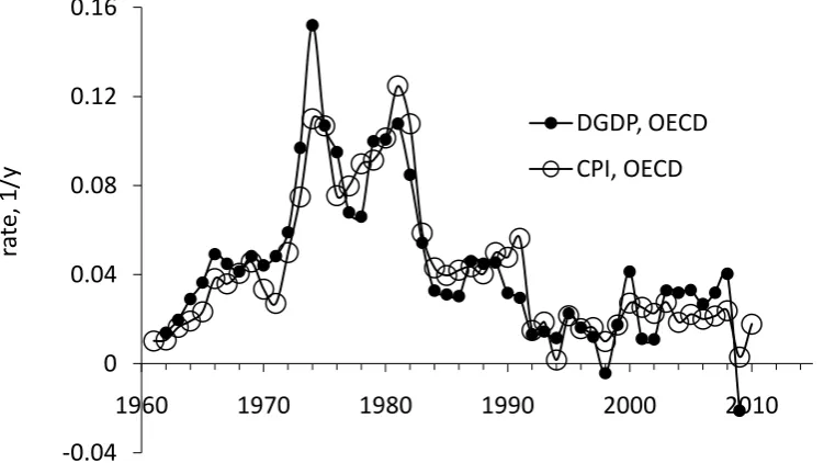
Figure 1 displays the evolution of two principal measures of price inflation – the GDP

deflator, DGDP, and consumer price index, CPI. Both variables were published by the OECD.

We presume the DGDP as a better representative of price inflation in a given country since it

includes all prices related to the economy. The overall consumer price index is fully included in

the DGDP and its behaviour is usually more volatile as representing only a (larger part) of the

economy. Since labour force and unemployment do characterize the entire economy it is

methodically correct to use the price deflator for quantitative modelling. Figure 1 shows that the

difference between the CPI and DGDP estimates can reach several percentage points and their

major peaks are not proportional in amplitude, e.g. 1974, 1982 and 1992. However, there are

periods of coherency.

Figure 1. Price inflation: comparison of CPI and the GDP deflator in Canada, both reported by the OECD.

For the period between 1962 and 2009 (48 readings) the mean rate of CPI inflation is

0.043y-1 (±0.031) and 0.044y-1 (±0.033) for the GDP deflator. Thus, the DGDP in Canada is

characterized by a higher volatility as associated with the peak in 1974. The rate of inflation fell

to the level of 0.04y-1 in the beginning of 1980s and then to 0.02y-1 in 1991, i.e. after the

introduction of inflation targeting. It has been oscillating around this level since. Between 1974

and 1983, inflation was almost everywhere above 6% per year. -0.04

0 0.04 0.08 0.12 0.16

1960 1970 1980 1990 2000 2010

ra

te,

1/

y

DGDP, OECD

Any macroeconomic variable is subject to measurement uncertainty and bias. Rossiter

(2005) has considered the bias in the Canadian CPI by examining four different potential

sources: commodity substitution bias, outlet substitution bias, quality change bias, and new

goods bias. He found that the total measurement bias has increased only slightly in recent years

to 0.6 percentage points per year (0.006y-1), and is low when compared with other countries.

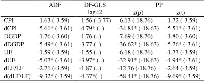
In order to establish a reliable link with the labour force, one needs to estimate basic

statistical properties of relevant time series. The order of integration can be determined using

unit root tests applied to the original series and their progressive differences. As a rule, the rate

of inflation in developed countries is an I(1) variable. Canada is not an exception, as Table 1

clearly demonstrates. In particular, we report the results of the following tests: the augmented

Dickey-Fuller (ADF), the DF-GLS, and the Phillips-Perron (PP) test. The DGDP series consists

of 48 readings (between 1962 and 2009) and the CPI series has 50 readings, both definitely

have a unit root. The first differences (dDGDP and dCPI) are characterized by the absence of

unit roots, and thus, the original time series is integrated of order 1. For the period between

1963 and 2009, the naive predictions of inflation at a one-year horizon have the standard

deviations of 0.020y-1 and 0.016y-1, respectively.

Table 1. Results of unit root tests for the original time series and their first differences.

ADF DF-GLS

lag=2

PP

z() z(t) CPI -1.63 (-3.59) -1.56 (-3.77) -6.13 (-18.76) -1.72 (-3.59) dCPI -5.61* (-3.61) -4.79* (..) -34.84* (-18.63) -5.51* (-3.61) DGDP -1.76 (-3.60) -1.76 (..) -7.69 (-18.70) -1.80 (-3.60) dDGDP -5.49* (-3.61) -3.77 (..) -36.62* (-18.63) -5.26* (-3.61) UE -1.59 (-3.59) -1.55 (..) -6.18 (-18.76) -1.77 (-3.59) dUE -5.07* (-3.61) -3.97* (..) -32.91* (-18.63) -4.94* (-3.61) dLF/LF -2.71 (-3.59) -1.87 (..) -12.76 (-18.76) -2.64 (-3.59) d(dLF/LF) -9.32* (-3.59) -4.37*(..) -58.41* (-18.76) -9.69* (-3.59)

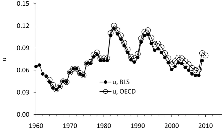
Figure 2 depicts two estimates of the rate of unemployment as reported by the OECD

and the U.S. BLS. Surprisingly, the difference between these curves is almost negligible, but

clearly demonstrates two artificial breaks in 1966 and 1976. There are two sharp peaks – in

1984 and 1994. The highest rate of unemployment in Canada was at the level of 11.4% (OECD

definition) in 1984, and the lowermost one was around 3.8% in 1967. Table 1 shows that the ut

series is likely integrated of order 1.

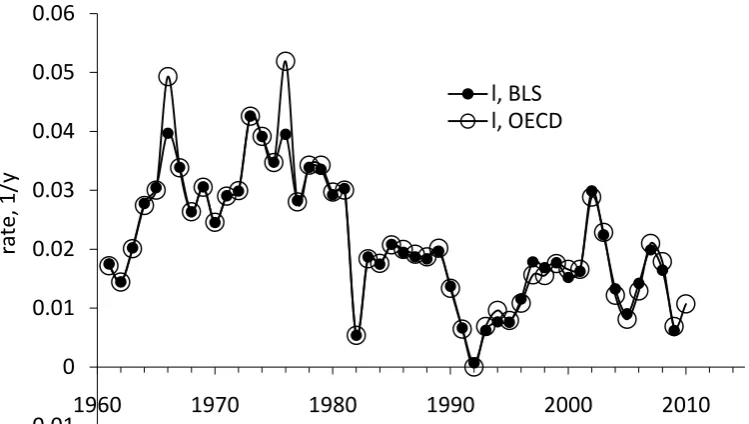
The rate of change in labour force, lt, in Figure 3 also has two representations: the

practically identical, except in 1967 and 1976. These are the years of revision to labour force

related definitions, with the spikes potentially damaging all LSQ-based statistical inferences.

Table 1 indicates that the annual estimates of labour force represent rather an I(1) process. The

augmented Dickey-Fuller and Phillips-Perron both reject the null hypothesis of a unit root.

However, the DF-GLS test does not reject the null for all lags above 1 (only lag 2 is shown in

the Table). The first difference, dlt, is an I(0) process with all tests rejecting the null hypothesis

of a unit root.

Figure 2. Comparison of two estimates of unemployment according to the U.S. BLS and OECD definitions.

Since linear functional dependences between the three involved I(1) processes are

estimated later on, econometric analysis requires specific tests for cointegration. We would not

like the results of our statistical estimates to be biased by stochastic trends, as was originally

found by Granger (1981) for various economic series.

The main task of this study is to accurately characterize in time and size the structural

break associated with the new monetary policy formally introduced in 1991. For this purpose,

we use the best fit empirical relationships between inflation/unemployment and labour force.

By definition, all relationships are linear and potentially lagged. Technically, this task does not

seem to be a difficult one since we use cumulative curves, accompanied by the residual

minimization in the L2-metric, instead of linear regression applied to the dynamic series. (The

latter method provides heavily biased estimates of the slope when both variables have high

uncertainties.) We have also tried using the L1-metrics as applied to the annual and cumulative

curves. However, the overall performance of the L2-metrics makes it a more appropriate for the

cumulative curves where large-amplitude outliers are almost absent. 0.00

0.03 0.06 0.09 0.12 0.15

1960 1970 1980 1990 2000 2010

u

Figure 3. Comparison of two estimates of the change rate of labour force level – as reported by the OECD and BLS.

2. Unemployment as a linear function of the change in labour force

In our previous paper on inflation/unemployment in Canada we demonstrated the absence of the

Phillips curve in its original form (Kitov 2007b). From the absent Phillips curve it is only one

little step to the dependence of unemployment on the change in labour force: we are looking for

a driving force. Actually, we replace the rate of inflation in the Phillips curve with the rate of

labour force change. Then, we have to estimate both coefficients in (2). The estimation method

is enhanced relative to our previous studies – the best overall fit is sought by the least squares

method as applied to the cumulative curves. In addition to the formal LSQ minimization of the

model error we have introduced a freely varying break year in the model. The break should be

within 4 years around the assumed year (1991). By definition, the final break year has to

provide the lowermost RMS residual. All in all, the best- fit equations and the break year are as

follows:

ut = -2.574lt + 0.155; t<1990

ut = -2.852lt + 0.122; t≥1990 (5)

with the break in 1990. The change in the break year is likely explained by the influence of

measurement noise. As an alternative, one may guess that the Bank of Canada introduced

inflation targeting in some testing regime a year before the official start. Figure 4 illustrates the

behaviour of the dynamic and cumulative curves. We have intentionally extended the model for

the period before 1990 into the 1990s and 2000s in order to demonstrate the structural break in

1990. The cumulative curves clearly deviate since 1990. -0.01

0 0.01 0.02 0.03 0.04 0.05 0.06

1960 1970 1980 1990 2000 2010

ra

te,

1/

y

In the previous paper, coefficients in (5) were as follows: b1=-2.1 and b2=-0.12. The

absolute value of the slope was underestimated since the original equation had to fit the whole

period between 1969 and 2004. The visual-fit approach and the absence of the structural break

made this task a difficult one. The intercept was estimated with a higher accuracy, at least after

1990. Overall, the original model gave a resonable first approximation.

Figure 4. Annual estimates of the rate of unemployment in Canada: measured vs. predicted from the change in labour force.

The slope in (5) is always negative. Therefore, any increase in the level of labour force

is reflected in a proportional and simultaneous fall in the rate of unemployment. This is a

fortunate link – more people in work force is equivalent to less unemployed. However, when

the level of labour force does not change with time the rate of unemployment is very high – 0.00

0.05 0.10 0.15 0.20

1960 1970 1980 1990 2000 2010

u

u, OECD

predicted with a structural break in 1990 predicted without structural breaks

0.0 1.0 2.0 3.0 4.0 5.0

1960 1970 1980 1990 2000 2010

u

u, OECD

around 12% (after 1990). Canada has to keep a higher rate of labour force growth in order to

retain the rate of unemplyment at low level.

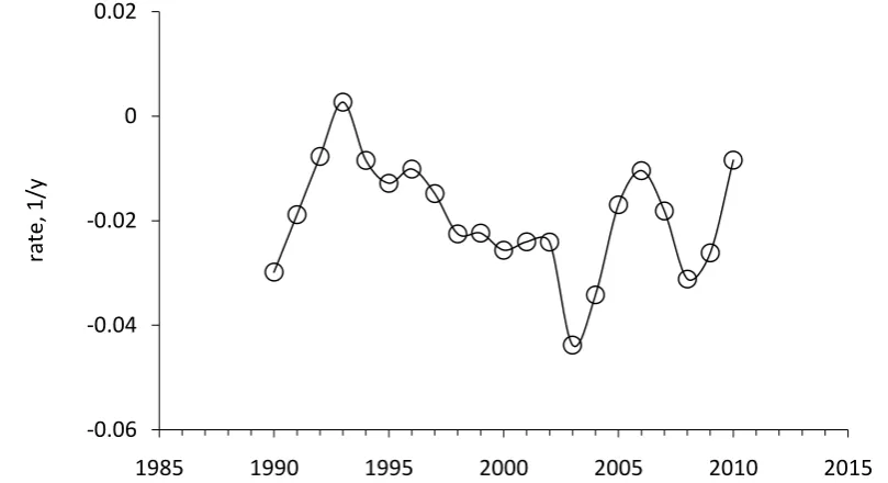
All in all, the model obtained for the previous period diverge after 1990. The difference

between the cumulative curves is positive and increases with time. This is a favourable

outcome of the new monetary policy – it has reduced the rate of unemployment by

approximately 3.6% relative to that predicted by the relationship valid before 1990 (see Figure

5). For the economic theory, it is likely an unexpected result since the Phillips curve implies an

opposite behaviour.

Figure 5. The difference between the observed rate of unemployment in Canada and that predicted by the relationship valid before 1990, i.e. the expected rate of unemployment.

Relationship (5) implies a nonlinear dependence on the rate of particiaption in labour

force. For a given absolute change in the level of labour force, the reaction of unemployment

will be different for the rate of participation 56% (1964) and 67.7% (2008). The higher is the

participation rate the lower is the change rate, lt, and thus, the change in the rate of

unemployment. Actually, the participation rate in Canada has been increasing since 1995 to a

very high level of 67.7%. It will be a difficult task to retain the rate of unemployment at the

current level – it is likely that the rate of participation is approaching the peak level and will

start to decline in the near future.

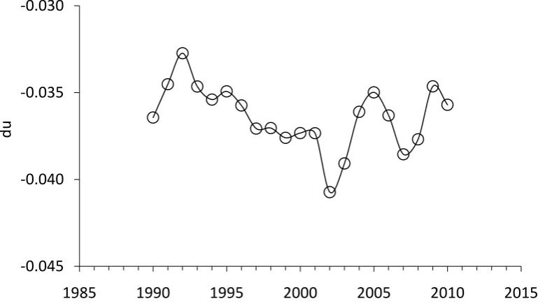
3. Inflation as a linear function of the change in labour force

The existence of a deterministic link between labour force and price inflation has also been

proved for many countries. We are following the same estimation procedure as for -0.045

-0.040 -0.035 -0.030

1985 1990 1995 2000 2005 2010 2015

unemployment above, i.e. the method of cumulative curves enhanced by the LSQ minimization

of the model error and the break year freely varying around 1991.

Figure 6. Modelling the annual and cumulative GDP deflator as a function of the change rate of labour force.

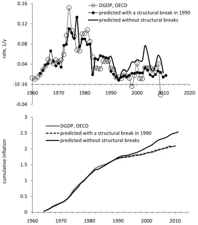
We start with annual readings of the GDP deflator reported by the OECD. The

minimization procedure with the start break year in 1991 (the change in monetary policy) and

zero lag (varied between zero and 5 years) has finally determined the data-driven break year in

1990 and the lag of 1 year:

DGDPt = 2.453lt-1 + 0.0052; t<1990

DGDPt = 0.842lt-1–0.0085; t≥1990 (6)

-0.04 -1E-16 0.04 0.08 0.12 0.16

1960 1970 1980 1990 2000 2010 2020

rate,

1

/y

DGDP, OECD

predicted with a structural break in 1990 predicted without structural breaks

0 0.5 1 1.5 2 2.5 3

1960 1970 1980 1990 2000 2010

cum

u

lati

ve

in

fl

a

ti

o

n

DGDP, OECD

Figure 6 displays the observed DGDP curve and that predicted according to (6). The

cumulative curves are in a good agreement. For the period between 1964 and 2009, the

coefficient of determination is very high: R2dyn=0.70 and R2cum= 0.999, respectively.

Relationship (6) does not use any past or future values of inflation (i.e. there are no AR terms)

which usually bring between 80% and 90% of the explanatory power in the mainstream models

(Piger and Rasche 2006; Rudd and Whelan 2005; Stock and Watson 2008). Hence, this link is

almost a deterministic one. The cumulative curves demonstrate that the left- and right-hand

sides in (6) converge with time.

Figure 7. The difference between the measured and expected GDP deflators. The mean value between

1990 and 2009 is -0.019y-1.

Figure 7 depicts another benefit of the new monetary policy - the rate of price inflation

has been reduced by 1.9% per year on average since 1991 relative to that predicted by the early

model. Hence, the policy has a significant effect on the price growth in Canada and the Lucas

critique was well justified by the reduced rate of unemployment. Unfortunately, this win-win

policy is not the only possible outcome of inflation targeting. In France, a similar (with strict

constraints on the level of money supply, however) monetary policy introduced in 1994 has

resulted in an opposite reaction of unemployment (Kitov 2007a). On average, the observed rate

has been approximately 5% above that predicted by the model valid before 1995. This was not a

win-win game.

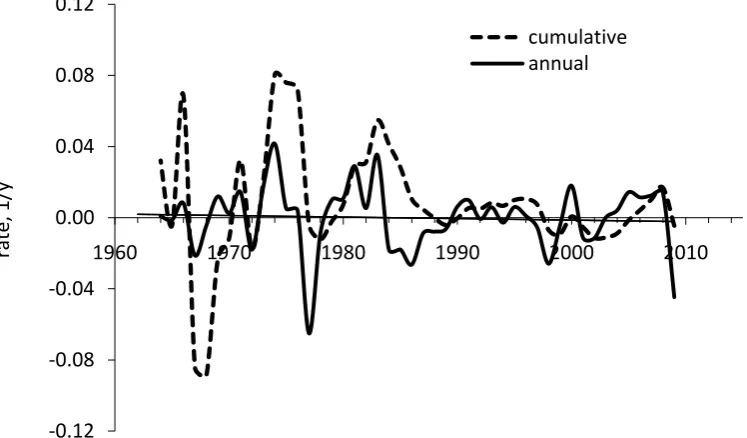
Figure 8 illustrates the expected benefits of the cumulative approach. The absolute and

relative errors decrease with time. Despite the annual levels of price and labour force are not

measured more accurately with time the relative change in the level is measured with an -0.06

-0.04 -0.02 0 0.02

1985 1990 1995 2000 2005 2010 2015

rate,

1

increasing accuracy due to the increasing denominator. As a consequence, the observed and

predicted cumulative curves, i.e. the overall changes in price and labour force, do converge.

They become indistinguishable. Taking into account the lead of the change in labour force by 1

year and its independence on the future rate of inflation one can suggest that there exists a

deterministic link between them.

Figure 8. Absolute dynamic and relative cumulative modelling error for the inflation in Figure 6.

The annual time series are relatively short with only 48 readings between 1962 and

2009. Small samples do not guarantee higher confidence of statistical results. However, we

have carried our formal tests for cointegration. First, we have tested the differences between the

dynamic and cumulative curves, i.e. the model residuals. For the annual residuals, the

augmented Dickey-Fuller test is -5.36 with the 1% critical value of -3.61, i.e. the null of a unit

root is rejected. The Phillips-Perron tests gives z()=-35.33* (-18.56) and z(t)=-5.23* (-3.61).

The DF-GLS test rejects the null for all lags between 1 and 5, except 4.

For the residuals of the cumulative model, the augmented Dickey-Fuller test is -4.16*

with the 1% critical value of -3.61. The Phillips-Perron tests gives z()=-26.05* (-18.56) and

z(t)=-4.18* (-3.61). The DF-GLS test rejects the null for all lags between 1 and 5, except 4.

Therefore, both residuals have no unit roots. This is an indication that the relevant measured

and predicted from labour force time series are likely cointegrated. Such a result for the

cumulative curves is not a surprising one – the residual error must have a zero mean despite

both series are integrated of order 2.

The Johansen test for cointegration supports the conclusion from the annual residual –

the annual measured and predicted curves are cointegrated. The trace statistics gives -0.12

-0.08 -0.04 0.00 0.04 0.08 0.12

1960 1970 1980 1990 2000 2010

ra

te,

1/

y

cointegration rank 1 for two variables. We used the following specifications: trend=”none”,

maxlag=3, but the outcome is the same for other trend specifications and maxlag=7. Formally,

the Johansen test cannot be applied to I(2) series and we did not test the cumulative curves.

As mentioned above, small samples usually do not provide statistical estimates and

inferences with the desired level of confidence. Fortunately, the OECD also reports quarterly

estimates of inflation and labour force. As a rule, monthly and quarterly data are noisy because

of measurement errors. For the Canadian time series the overall measurement accuracy is not

poor and we have obtained the estimates of coefficients in the linear link between the annual

change rate of the GDP deflator for each quarter (annualized Q/Q) and lt:

DGDPt = 3.0lt-8–0.0045; t≥1989

DGDPt = 2.0lt-8–0.0020; t≤1989 (7)

where the lag is 8 quarters and the break year is 1989. The change in the lag and break is

likely associated with extremely high volatility of quarterly estimates. Thus, this model is a

crude one. The change in monetary policy did introduce a tangible disturbance in the link

between inflation and labour force. Figure 9 presents the quarterly curves for observed and

predicted inflation, both smoothed with MA(8). The resemblance is relatively good.

Figure 9. Modelling the quarterly DGDP estimates, both curves are smoothed with MA(8).

We have tested the smoothed time series for cointegration. In the Engle-Granger test for

cointegration, the residual error of linear regression should not have unit roots. Figure 10

depicts the model residual, which we consider as an equivalent of the regression residual error. -0.005

0 0.005 0.01 0.015 0.02 0.025 0.03 0.035

1960 1970 1980 1990 2000 2010 2020

rate,

1

/y

For 188 readings, the augmented Dickey-Fuller (DF) test z(t)=-4.37* with the 1% critical value

of -3.48. The DF-GLS test rejects (for 1% critical value) the null of a unit root for lags 1, 5 and

6 (quarters). The Phillips-Perron test for unit roots gave z()=-35.95* and z(t)=-4.50*, with the

1% critical value of -20.07 and -3.48, respectively. Therefore, all tests for unit roots prove that

the predicted time series is cointegrated with the observed one. The Johansen test confirms the

presence of a cointegration relation. Econometrically, there exists a long term equilibrium

relation between the rate of inflation and the change in labour force in Canada with a break

around 1990. This makes the above results of linear regression unbiased.

Figure 10. The model residual from Figure 9.

The overall consumer price index allows corroboration of the results obtained for the

GDP deflator. We apply the same technique to the annual readings of CPI inflation reported by

the OECD. The minimization procedure with the start break year in 1991 (the change in

monetary policy) and zero lag (varied between zero and 5 years) has finally determined the

data-driven break year in 1991 and the lag of 3 years:

CPIt = 2.682lt-3 - 0.0035; t<1991

CPIt = 0.625lt-3 + 0.0104; t≥1991 (7)

Considering the difference between DGDP and CPI in Figure 1 the change in lag is not a

surprise. At the same time, the break year fits the introduction of inflation targeting. Figure 11

depicts the annual and cumulative curves; the latter also includes a model without structural

break. The annual curves are smoothed with MA(3) and demonstrate a very high degree of -0.02

-0.01 0.00 0.01 0.02

1960 1970 1980 1990 2000 2010

ra

te,

1/

similarity for the period between 1964 an 2010 with R2=0.89. For the annual estimates, R2=0.68

and for the cumulative ones R2=0.999. These estimates are not bogus when the annual time

series are cointegrated.

Figure 11. Modelling the annual and cumulative CPI inflation as a function of the change rate of labour force. The structural break was found in 1991. Both annual curves are smoothed with MA(3).

There are 47 readings between 1964 and 2010. We have tested the differences between

the dynamic and cumulative curves, i.e. the model residuals, for unit roots. For the annual

residuals, the augmented Dickey-Fuller test is -5.83* with the 1% critical value of -3.61, i.e. the

null of a unit root is rejected. The Phillips-Perron tests gives z()=-31.83* (-18.63) and z(t)

=-5.78* (-3.61). The DF-GLS test rejects the null for all lags between 1 and 5. Hence, there is no

unit root in the model residual, i.e. the rate of CPI inflation and the change in labour force are 0

0.04 0.08 0.12 0.16

1960 1970 1980 1990 2000 2010

ra

te,

1/

y

CPI

predicted with a structural break in 1990

0 0.5 1 1.5 2 2.5 3

1960 1970 1980 1990 2000 2010

cu

mu

la

ti

ve

in

fl

a

ti

on

CPI

cointegrated, when one introduces a structural break in the cointegrating relation in 1991. The

Johansen test gives rank 1 and confirms the presence of one cointegrating relation between the

measured and predicted inflation. The driving force leads by 3 years creating a natural forecast

horizon of the same length. The standard deviation in the predicted series (i.e. a

three-year-ahead inflation estimate) is 0.024y-1. This value is smaller than the RMSE of the naïve

prediction (Atkeson and Ohanian 2001) at the same 3-year horizon, 0.028y-1. When one

smoothes the predicted inflation series with MA(3) the forecast horizon falls to 2 years. Then

the RMSFE of our model is only 0.018y-1 compared to 0.023y-1 for the naïve prediction at a 2

-year horizon.

Taking into account the cointegrating relations estimated for the DGDP and CPI series

one can conclude that the change in labour force has been driving inflation (at least) since the

beginning of 1960s. The structural break associated with the introduction of inflation targeting

definitely induced shifts in all coefficients, but did not change the linear functional dependence

and the lag of inflation. This finding may be interpreted as a shift from one stationary regime of

the Canadian economy to another regime, also a stationary one.

All in all, the new monetary policy has affected inflation and unemployment, and both

in a desired direction. This confirms the correctness of the Lucas critique. However, both

variables are still driven by the change in labour force. Moreover, the joint effect of inflation

targeting is zero when the generalized model is applied, i.e. the change in unemployment is

fully compensated by the change in inflation a year (or three years) later when equation (3) or

(4) is applied.

4. The generalized model

In Sections 2 and 3, we have estimated several individual links between labour force,

unemployment and inflation. Both individual relations to labour force are cointegrated, as the

Engle-Granger and Johansen tests have shown. However, there was a structural break in 1991

induced by the introduction of new monetary policy. In this case, the estimation of a

generalized model is a mandatory one. Since inflation lags behind the rate of unemployment

and the change in labour force we have estimated model (4) for DGDP and CPI separately:

DGDPt = 3.70lt-1 + 0.55ut-1 - 0.076

CPIt = 3.40lt-3 + 0.55ut-3 - 0.073 (8)

Coefficients in (8) are similar for both measures of inflation with a little higher influence of

compensated by a slightly lower intercept of -0.076. The influence of unemployment is

essentially the same. The most important finding is that there is no sign of the 1991 structural

break in (8) and one equation covers the entire period between 1965 and 2010. This is an

obvious consequence of the balance between inflation and unemployment in (8). When the rate

of unemployment falls by 3.6% per year the rate of inflation also drops by 0.55*3.6%= 2%. The

estimated value of inflation fall after 1991 is 1.9% per year.

Figure 12. Upper panel: Illustration of the generalized relation between inflation, unemployment and the

change rate of labour force level in Canada. The GDP deflator is modelled using the change rate of

labour force level and unemployment. Both series are smoothed with MA(3). Lower panel: These

cumulative curves were used to estimate all coefficients in (8).

Figures 12 and 13 present the measured and predicted inflation. The annual series are

characterized by R2=0.52 in both cases. In Figure 12, we have smoothed the annual curves with -0.05

0 0.05 0.1 0.15

1960 1970 1980 1990 2000 2010

ra

te,

1/

y

DGDP, OECD

predicted

0.0 0.5 1.0 1.5 2.0 2.5

1960 1970 1980 1990 2000 2010

cu

mu

la

ti

ve

in

fl

a

ti

on

DGDP, OECD

MA(3) and the curves are very close to each other. The difference between the annual series

has no unit roots as the augmented Dickey-Fuller (-5.48*) and the Phillips-Perron (z(ρ)=-34.47* and z(t)=-5.47*) tests show. Thus, there is no unit root in the model residual.

Figure 13. Upper panel: Illustration of the generalized relation between inflation, unemployment and the

change rate of labour force level in Canada. The CPI inflation is modelled using the change rate of

labour force level and unemployment. Lower panel: These cumulative curves were used to estimate all

coefficients in (8).

In Figure 13, we did not smooth the annual curves in order to demonstrate the reason for

a relatively low R2. As discussed in Section 1, there are artificial breaks in the units of labour

force and unemployment measurements in 1967 and 1976. One can also suggest that there was

a major revision in 1982. After 2005, there is a high-amplitude oscillation potentially

catastrophic for any quantitative modelling. All these spikes deteriorate the result of linear -0.05

0 0.05 0.1 0.15 0.2

1960 1970 1980 1990 2000 2010

ra

te,

1/

y

CPI, OECD

predicted

0 0.5 1 1.5 2 2.5

1960 1970 1980 1990 2000 2010

cu

mu

la

ti

ve

in

fl

a

ti

on

CPI, OECD

regression. However, there is no unit root in the difference between the observed and predicted

rate of inflation, as the ADF (-5.47*) and the PP (-35.78* and -5.49*) tests demonstrate.

Conclusion

The Lucas critique was correct. The manipulations associated with the introduction of the new

monetary policy in 1991 produced a substantial effect on the long-term equilibrium relation

between the rate of price inflation and the change in labour force. Amazingly, the monetary

policy had a highly positive side effect of a lowered unemployment. In 2010, the rate of

unemployment would be around 12% without the inflation targeting. In France, the effect of a

similar monetary policy, adapted by the Banque de France in 1995, is opposite – lowered price

inflation resulted in the rate of unemployment as high as 12% or ~5 percentage points above the

rate without the new policy (Kitov 2007a).

All in all, the rate of price inflation and unemployment in Canada is a one-off function

of the change in labour force. This conclusion validates the previous model for Canada and the

models for many developed countries: the U.S., Japan, Germany, France, Italy, Canada, the

Netherlands, Sweden, Austria, and Switzerland.

Overall, we have established that there exist long term equilibrium relations between the

rate of labour force change and the rate of inflation/unemployment. The level of statistical

significance of these cointegrating relations in the absence of AR-terms allows us to consider

these links as deterministic ones, as adapted in physics. This does not make the rate of

unemployment and inflation non-stochastic time series. The change in labour force includes a

strong demographic component, and thus, is stochastic to the extent the evolution of population

in a given country is stochastic. Since the level of labour force is a measurable value one does

not need a data generating process in order to describe its stochastic properties – they are

obtained automatically with routine measurements.

References

Atkeson, A., & Ohanian, L. (2001). Are Phillips Curves Useful for Forecasting Inflation? Federal

Reserve Bank of Minneapolis Quarterly Review, 25(1), 2–11.

Bank of Canada. (2010). Monetary policy. Retrieved 26.03.2011, http://www.bank-banque-canada.ca/en/monetary/inflation_target.html

Benati, L. (2009). Are “intrinsic inflation persistence” models structural in the sense of Lucas (1976)?

ECB Working paper series, No 1038.

Binette, A., Martel, S. (2005). Inflation and Relative Price Dispersion in Canada: An Empirical Assessment, Bank of Canada, Working Paper 2005-28, Ottawa

Bureau of Labor Statistic. (2007). Foreign Labor Statistic. Table, retrieved at 20.07.2007 from http://data.bls.gov/PDQ/outside.jsp?survey=in

Granger, C. (1981). Some Properties of Time Series Data and Their Use in Econometric Model

Specification, Journal of Econometrics 16, 121-130.

Hostland, D. (1995). Changes in the inflation process in Canada: Evidence and implications, Bank of

Canada, Working paper 95-5, Ottawa

Kitov, I. (2006). Inflation, unemployment, labour force change in the USA. Working Papers 28,

ECINEQ. Society for the Study of Economic Inequality

Kitov, I. (2007a). Inflation, Unemployment, Labour Force Change in European countries. In T.

Nagakawa (Ed.), Business Fluctuations and Cycles (pp. 67-112). Hauppauge NY: Nova Science

Publishers.

Kitov, I. (2007b). Exact prediction of inflation and unemployment in Canada, MPRA Paper 5015, University Library of Munich, Germany

Kitov, I., & Kitov, O. (2008). The Driving Force of Labor Force Participation in Developed Countries.

Journal of Applied Economic Sciences, III(3(5)_Fall), 203-222. Spiru Haret University, Faculty

of Financial Management and Accounting Craiova.

Kitov, I., & Kitov, O. (2010). Dynamics of Unemployment and Inflation in Western Europe: Solution by

the 1-D Boundary Elements Method. Journal of Applied Economic Sciences, V(2(12)_Summer),

94-113. Spiru Haret University, Faculty of Financial Management and Accounting Craiova. Kitov, I., Kitov, O., & Dolinskaya, S. (2007). Inflation as a function of labour force change rate:

cointegration test for the USA. MPRA Paper 2734. University Library of Munich, Germany.

Lucas, R. (1976). Econometric policy evaluation. A critique. Cornegie-Rochester Conference Series on

Public Policy, 1, 19-46.

Page, E. S. (1954). Continuous Inspection Scheme. Biometrika41 (1/2): 100–115.

Phillips, A. W. (1958). The Relationship between Unemployment and the Rate of Change of Money

Wages in the United Kingdom 1861-1957. Economica25 (100), 283–299.

Piger, J., & Rasche, R. (2006). Inflation: do expectations trump the gap? Working Papers 2006-013.

Federal Reserve Bank of St. Louis.

Rossiter, J. (2005) Measurement Bias in the Canadian Consumer Price Index. Bank of Canada, Working Paper 2005-39, Ottawa

Rudd, J., & Whelan, K. (2005). New Tests of the New-Keynesian Phillips Curve. Journal of Monetary

Economics, 52(6), 1167–1181.

Statistics Canada. (2011). History of the Labour Force Survey prior to November 2000. Retrieved 27.03.2011, http://www.statcan.gc.ca/imdb-bmdi/document/3701_D7_T9_V1-eng.pdf

Stock, J., & Watson, M. (2003). Forecasting Output and Inflation: The Role of Asset Prices. Journal of

Economic Literature 41(3), 788–829.

Stock, J., & Watson, M. (2007). Why has U.S. inflation become harder to forecast? Journal of Money,

Credit and Banking, 39(1), 3-34.

Stock, J., & Watson, M. (2008). Phillips Curve Inflation Forecasts. NBER Working Papers 14322.