Least Squares Solution for Discrete Time Nonlinear Stochastic Optimal Control Problem with Model Reality Differences

(1)

http://www.scirp.org/journal/am ISSN Online: 2152-7393 ISSN Print: 2152-7385

Least Squares Solution for Discrete Time

Nonlinear Stochastic Optimal Control Problem

with Model-Reality Differences

Sie Long Kek

1

, Jiao Li

2

, Kok Lay Teo

3

1_{Center for Research on Computational Mathematics, Universiti Tun Hussein Onn Malaysia, Batu Pahat, Malaysia} 2_{School of Mathematics and Computing Science, Changsha University of Science and Technology, Changsha, China} 3_{Department of Mathematics and Statistics, Curtin University of Technology, Perth, Australia}

Abstract

In this paper, an efficient computational approach is proposed to solve the discrete time nonlinear stochastic optimal control problem. For this purpose, a linear quadratic regulator model, which is a linear dynamical system with the quadratic criterion cost function, is employed. In our approach, the mod-el-based optimal control problem is reformulated into the input-output equa-tions. In this way, the Hankel matrix and the observability matrix are con-structed. Further, the sum squares of output error is defined. In these point of views, the least squares optimization problem is introduced, so as the differ-ences between the real output and the model output could be calculated. Ap-plying the first-order derivative to the sum squares of output error, the neces-sary condition is then derived. After some algebraic manipulations, the op-timal control law is produced. By substituting this control policy into the in-put-output equations, the model output is updated iteratively. For illustration, an example of the direct current and alternating current converter problem is studied. As a result, the model output trajectory of the least squares solution is close to the real output with the smallest sum squares of output error. In con-clusion, the efficiency and the accuracy of the approach proposed are highly presented.

Keywords

Least Squares Solution, Stochastic Optimal Control, Linear Quadratic Regulator, Sum Squares of Output Error, Input-Output Equations

1. Introduction

Stochastic dynamical system is a practical system in modeling and simulating How to cite this paper: Kek, S.L., Li, J. and

Teo, K.L. (2017) Least Squares Solution for Discrete Time Nonlinear Stochastic Op-timal Control Problem with Model-Reality Differences. Applied Mathematics, 8, 1-14.

http://dx.doi.org/10.4236/am.2017.81001

Received: November 17, 2016 Accepted: January 8, 2017 Published: January 11, 2017

http://creativecommons.org/licenses/by/4.0/

(2)

the real-world problems. The behavior of the fluctuation, which is caused by the effect of noise disturbance in the dynamical system to represent the real

situa-tion, rises to the attention of many researchers. See for examples, [1]-[8]. As

such, optimization and control of the stochastic dynamical system are a chal-lenging topic. In the past decades, the research outcomes, both for theoretical

results and development of the algorithms, are well-defined [9] [10] [11] [12]

[13]. In general, the real processes, which are modeled into the stochastic

optim-al control problem, are mostly nonlinear process. Their actuoptim-al models in naturoptim-al could be necessary unknown. Applying the linear model, including the Kalman filtering theory, to solve the stochastic optimal control problems, in particular, for nonlinear case, give a simplification methodology instead [14][15][16][17].

Recently, the integrated optimal control and parameter estimation (ICOPE) algorithm, which solves the linear model-based optimal control problem itera-tively, is proposed in the literature [18][19]. The purpose of this algorithm is to provide the optimal solution of the discrete time nonlinear stochastic optimal control problem with the different structure and parameters. In this algorithm, the adjusted parameters are added into the model used so as the differences be-tween the real plant and the model used can be calculated, in turn, update the optimal solution of the model used during the computation procedure. The in-tegration of system optimization and parameter estimation is the main feature of this algorithm, where the principle of model-reality differences and the Kalman filtering theory are incorporated. Once the convergence is achieved, the iterative solution approximates to the correct optimal solution of the original optimal control problem, in spite of the model-reality differences. However, increasing the accuracy of the model output to track the real output would be necessary required.

In this paper, an efficient matching scheme, which diminishes the adjusted parameters, is established deliberately. In our approach, the model-based optim-al control problem is simplified from the discrete-time nonlinear stochastic op-timal control problem. Then, this model-based opop-timal control problem is re-formulated into the input-output equations. During the formulation of the in-put-output equations, the Hankel matrix and the observability matrix are con-structed. These matrices capture the characteristic of the model used into the output measurement. By virtue of this, the least square optimization problem is introduced. From the validation of the first order necessary condition, the nor-mal equation is resulted and the optinor-mal control law is updated accordingly on the recursion formula. As a result of this, the sum squares of the output error could be minimized demonstratively. Hence, the efficiency of the algorithm proposed is highly presented.

(3)

prob-lem is illustrated and the result is demonstrated. Finally, some concluding re-marks are made.

2. Problem Description

Consider a general class of dynamical system given by

(

1

)

(

( ) ( )

, ,

)

( )

x k+ = f x k u k k +Gω k (1a)

( )

(

( )

,

)

( )

y k =h x k k +η k (1b)

where _{u k}

( )

_{∈ ℜ}m, 0,1,_k₌ _,_N₋1, _{x k}

( )

_{∈ ℜ}n, 0,1,_k₌ _,_N, and

( )

p, 0,1, ,

y k ∈ ℜ k=  N, are, respectively, the control sequence, the state

se-quence and the output sese-quence. The terms ω

( )

k ∈ ℜq, 0,1,k= ,N−1, and

( )

k p, 0,1,k ,N

η ∈ ℜ =  , are, respectively, process noise sequences and output

noise sequences. Both of these noise sequences are the stationary Gaussian white

noise sequences with zero mean and their covariance matrices are given by Q_ω

and R_η, respectively, where Q_ω is a q×q positive definite matrix and R_η is

a p×p positive definite matrix. In addition, G is an n×q process noise

coefficient matrix, f :ℜ × ℜ × ℜ → ℜn m n represents the plant dynamics and

: n p

h ℜ × ℜ → ℜ is the output measurement channel.

Here, the aim is to find the control sequence u k

( )

, 0,1,k= ,N−1, such

that the following cost function

( )

(

( )

)

1

(

( ) ( )

)

0

, , ,

N

k

g u E ϕ x N N L x k u k k

−

=

 

= _ + _



∑

 (2)

is minimized over the dynamical system in Equation (1), where ϕ ℜ × ℜ → ℜ: n

is the terminal cost and L:ℜ × ℜ × ℜ → ℜn m is the cost under summation. The

cost function g0 is the scalar function and E

[ ]

⋅ is the expectation operator. It

is assumed that all functions in Equations (1) and (2) are continuously differen-tiable with respect to their respective arguments.

The initial state is

( )

0 0

x =x

where 0

n

x ∈ℜ is a random vector with mean and variance given, respectively,

by

[ ]

0 0

E x =x and E

(

x0−x0

)(

x0−x0

)

T=M0.

Here, M0 is an n n× positive definite matrix. It is assumed that the initial

(4)

( )

( ) ( ) ( )

(

( )

)

1

T T T

1

0

1 1

min

2 2

N

u k

k

g u x N S N x N x k Qx k u k Ru k

−

=

= +

∑

+

subject to (3)

(

1

)

( )

,

x k+ = Ax k +Bu k x

( )

0 =x0

( )

y k =Cx k

where x k

( )

∈ ℜn, 0,1,k= ,N , and y k

( )

∈ ℜp, 0,1,k= ,N, are,

respec-tively, the expected state sequence and the expected output sequence. Here, A

is an n n× state transition matrix, B is an n m× control coefficient matrix,

C is a p×n output coefficient matrix, whereas S N

( )

and Q are n n×

positive semi-definite matrices, R is a m m× positive definite matrix and g1

is the scalar cost function.

Notice that only solving Problem (M) actually would not give the optimal so-lution of Problem (P). However, by establishing an efficient matching scheme, it is possible to approximate the true optimal solution of Problem (P), in spite of model-reality differences. This could be done iteratively.

3. System Optimization with Least Square Updating Scheme

Now, let us define the Hamiltonian function for Problem (M) as follows:

( )

1

(

( )

T

( ) ( )

T

( )

)

(

)

T

(

( )

)

1 2

H k = x k Qx k +u k Ru k + p k+ Ax k +Bu k . (4)

Then, from Equation (3), the augmented cost function becomes

( )

( ) ( ) ( )

( ) ( )

(

( )

( ) ( )

)

T T

1

T T

0

1

0 0

2

N

k

g u x N S N x N p x

p N x N H k p k x k

−

=

′ = +

− +

∑

− (5)

where

( )

n

p k ∈ ℜ is the appropriate multiplier to be determined later.

Applying the calculus of variation [20] [21][22] to the augmented cost

func-tion in Equafunc-tion (5), the following necessary condifunc-tions are resulted: 1) Stationary condition:

( )

T

(

1

)

0

H k

Ru k B p k u k

∂

= + + =

∂ (6)

2) Costate equation:

( )

T

(

1

)

( )

H k

Qx k A p k p k

x k ∂

= + + =

∂ (7)

3) State equation:

( )

(

1

)

( )

(

1

)

H k

Ax k Bu k x k p k

∂

= + = +

∂ + (8)

with the boundary conditions x

( )

0 =x0 and p N

( )

=S N x N

( ) ( )

.

3.1. State Feedback Optimal Control Law

(5)

can be used in solving Problem (M).

Theorem 1. For the given Problem (M), the optimal control law is the feed-back control law defined by

( )

( ) ( )

u k = −K k x k (9)

where

( )

(

_T

(

)

1 _T

(

)

1 1

K k = B S k+ B+R − B S k+ A (10)

( )

T

(

)

(

( )

)

1

S k =A S k+ A−BK k +Q (11)

with the boundary condition S N

( )

given. Here, the feedback control law is a

linear combination of the states. That is, the optimal control is linear state-vari- able feedback.

Proof. From Equation (6), the stationary condition can be rewritten as

( )

T

(

₁

)

Ru k = −B p k+ . (12)

Applying the sweep method [20][21][22],

( )

( ) ( )

p k =S k x k , (13)

for k= +k 1 in Equation (12) to yield

( )

T

(

) (

)

1 1

Ru k = −B S k+ x k+ . (14)

Taking Equation (8) into Equation (14), we have

( )

T

(

₁

)

(

( )

)

Ru k = −B S k+ Ax k +Bu k .

After some algebraic manipulations, the feedback control law (9) is obtained, where Equation (10) is satisfied.

Now, substituting Equation (13) for k= +k 1 into Equation (7), the costate

equation is written as

( )

T

(

₁

) (

₁

)

p k =Qx k +A S k+ x k+ (15)

and considering the state Equation (8) in Equation (15), the costate equation becomes

( )

T

(

₁

)

(

( )

)

p k =Qx k +A S k+ Ax k +Bu k . (16)

Hence, by applying the feedback control law (9) in Equation (16), and doing some algebraic manipulations, it could be seen that Equation (11) is satisfied af-ter comparing the manipulation result to Equation (13). This completes the proof.

By substituting Equation (9) into Equation (8), the state equation becomes

(

1

)

(

( )

)

( )

x k+ = A−BK k x k (17)

and the model output is measured from

( )

y k =Cx k . (18)

In view of this, the calculation procedure for obtaining the feedback control law for Problem (M) is summarized below:

(6)

Step 0 Calculate K k

( )

, 0,1,k= ,N−1 , and S k

( )

, 0,1,k= ,N , from

Equations (10) and (11), respectively.

Step 1 Solve Problem (M) that is defined by Equation (3) to obtain

( )

, 0,1, , 1

u k k=  N− , and x k

( ) ( )

, , 0,1,y k k= ,N , respectively, from

Equations (9), (17) and (18).

Step 2 Evaluate the cost function g1 from Equation (3).

Remarks:

1) Data A, B, C can be obtained by the linearization of the real plant f and

the output measurement h from Problem (P).

2) In Step 0, the offline calculation is done for K k

( )

, 0,1,k= ,N−1, and

( )

, 0,1, ,

S k k=  N.

3) The solution procedure, which the dynamical system is solved in Step 1, and the cost function is evaluated in Step 2, is known as system optimization.

3.2. Least Squares Updating Scheme

Now, we define the output error : m p

r ℜ → ℜ given by

( )

,

r u =y k −y k (19)

where the model output (18) is reformulated as

( )

y k =Cx k +Du k . (20)

where D is a p×m coefficient matrix. Formulate Equation (20) as the

fol-lowing input-output equations [23] for k=0,1,,N:

( )

(

)

2 0

1 2 3

0 0 0 0 0

1 0 0 1

.

2 0 2

1

N N N N

y C D u

y CA CB D u

x

y CA CAB CB D u

y N CA CA −B CA − B CA − B D u N

                      =  +                   _ _ _ _ ₋                  (21)

For simplicity, we have

0

y=Ex +Fu (22)

where 2 N C CA E CA CA         =          and

1 2 3

0 0 0

0 0

. 0

N N N

D

CB D

F CAB CB D

CA −B CA − B CA − B D

        =                 

In addition, define the objective function 2:

m

g ℜ → ℜ, which represents the

sum squares of error (SSE), given by

( )

( ) ( )

T 2

g u =r u r u . (23)

Then, an optimization problem, which is referred to as Problem (O), is stated as follows:

(7)

Find a set of the control sequence u k

( )

, 0,1,k= ,N−1, such that the

ob-jective function g2 is minimized.

It is obviously noticed that for solving Problem (O), Taylor’s theorem [24]

[25] is applied to write the objective function g2 as the second-order Taylor

expansion about the current ( )i

u at iteration i as follows:

( )

(

( ) ( )

)

( )

( ) ( ) ( )

(

)

(

( )

)

(

( ) ( )

)

T 1 1

2 2 2

T

1 2 1

2

1

2

i i i i i

g u g u u u g u

u u g u u u

+ +

≈ + − ∇

+ − ∇ − (24)

where the higher-order terms are ignored and the notation ∇ represents the

differential operator. The first-order condition in Equation (24) with respect to

( )i1

u + is expressed by

( )

(

2

( )

)

(

( )1 ( )

)

2 2

0≈ ∇g ui + ∇ g ui ui+ −ui . (25)

Rearrange Equation (25) to yield the normal equation,

( )

(

2

)

(

( )1 ( )

)

( )

2 2

i i i i

g u u + u g u

∇ − = −∇ . (26)

Notice that the gradient ∇g2 is calculated from

( )

( ) T

( )

2 2

i i i

g u r u r u

∇ = ∇ (27)

and the Hessian of g2 is computed from

( )

( ) T

( )

( ) T

( )

2 2

i i i i i

g u  r u r u r u r u 

∇ = ∇ + ∇ ∇ 

  (28)

where

( )

( )i

r u

∇ is the Jacobian matrix of

( )

( )i

r u , and its entries are denoted

by

( )

(

i

)

i

( )

( )i _{, 1, 2,} _, _{1; 1, 2,} _, _1. ij

j

r

r u u F i N j N

u

∂

∇ = = = − = −

∂   (29)

From Equations (27) and (28), Equation (26) can be rewritten as

( )

T

( )

( ) T

( )

(

( ) ( )

)

( )

( ) T

( )

1

2 i i i i i i i i _.

r u r u r u r u u + u r u r u

_∇ _{+ ∇} _∇  ₋ _{= −∇}

 

  (30)

By ignoring the second-order derivative term, that is, the first term at the left-hand side of Equation (30), and define

( ) ( )1 ( )

-i i i

u u + u

∆ = _{, (31)}

the normal equation given by Equation (26) is simplified to

( )

T

( )

( ) ( )

( )

( ) T

( )

i i i i i

r u r u u r u r u

_∇ _∇ _∆ _{= −∇}

 

  . (32)

Then, we obtain the following updating recurrence relation,

( )i1 ( )i ( )i

u + =u + ∆u (33)

with the initial ( )0

u given, where

( )

( ) T

( )

( ) 1

( )

( ) T

( )

i i i i i

u r u r u r u r u

−

   

∆ = − ∇_ ∇ _{ }∇ _

(8)

Hence, Equations (33) and (34) are known as the least squares recursive equa-tions, which are based on the Gauss-Newton recursion formula.

From the discussion above, the least-squares updating scheme for the control sequence is summarized below:

Algorithm 2: Least-squares updating scheme Step 0 Given an initial ( )0

u and the tolerance ε. Set i=0.

Step 1 Evaluate the output error

( )

( )i

r u and the Jacobian matrix ∇r u

( )

( )i

from Equations (19) and (29), respectively.

Step 2 Solve the normal equation from Equation (32) to obtain ( )i

u

∆ _.

Step 3 Update the control sequence by using Equation (33). If ( )i1 ( )i

u + =u ,

within a given tolerance ε, stop; else set i= +i 1 and repeat from Step 1 to

Step 3. Remarks:

1) In Step 1, the calculation of the output error

( )

( )i

r u and the Jacobian

ma-trix

( )

( )i

r u

∇ are done online, however, the Jacobian matrix

( )

( )i

r u

∇ could

be done offline if it is independent from ( )i

u .

2) In Step 2, the inverse of

( )

( ) T

( )

i i

r u r u

∇ ∇ must be exist, and the value of

( )i

u

∆ _{represents the step-size for the control set-point.}

3) In Step 3, the initial ( )0

u is calculated from (9). The condition u( )i+1 =u( )i

is required to be satisfied for the converged optimal control sequence. The fol-lowing 2-norm is computed and it is compared with a given tolerance to verify the convergence of u k

( )

:

( ) ( ) 1

_{( )}

( )

_{( )}

( ) 1 2 1

1

0

N

i i

k

u u u k u k

− ₊

+

=

 

− =_ − _



∑

 . (35)

4) In order to provide a convergence mechanism for the state sequence, a simple relaxation method is employed:

( )i 1 ( )i

(

( )i

)

x

x + =x +k x−x (36)

where kx∈

(

0,1

]

, and x is the state sequence of the real plant.

4. Illustrative Example

In this section, an example of the direct current and alternating current (DC/AC)

converter model is illustrated [26] [27] [28]. In this model, the real plant is a

nonlinear dynamics structure and the output channel is a single output mea-surement, where the stationary Gaussian white noises are taken into the model. Since this model is a continuous time model, the simple discretization scheme is required. We define this model as Problem (P), while the simplified model, which is an expectation model, is employed as Problem (M). The cost function for both problems is a quadratic criterion function. The true solution of the original optimal control problem would be obtained by using the approach pro-posed and the solution procedure is implemented in the MATLAB environment.

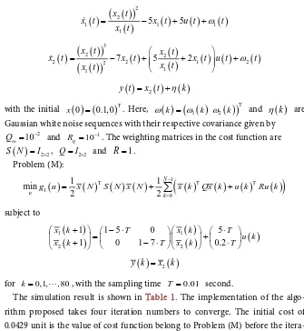
Problem (P):

( )

( ) ( ) ( )

1

(

( )

)

T T T

0

1 1

min

2 2

N

u

k

g u E x N S N x N x k Qx k u k Ru k

−

=

 

= _ + + _

(9)

subject to

( )

(

( )

_{( )}

)

( )

2 2

1 1 1

1

5 5

x t

x t x t u t t

x t ω

= − + + 

( )

(

( )

)

( )

(

)

( )

( ) ( )

( )

3 2 2

2 2 2 1 2

1 1

7 5 2

x t x t

x t x t x t u t t

x t x t

ω

  = − +_ + _ +   

( )

2

( )

y t =x t +η k

with the initial

( ) (

)

T

0 0.1, 0

x = . Here, ω

( )

k =

(

ω₁

( )

k ω₂

( )

k

)

T and η

( )

k are

Gaussian white noise sequences with their respective covariance given by

2

10

Q_ω = − and _R ₁₀1

η = − . The weighting matrices in the cost function are

( )

2 2

S N =I× , Q=I2 2× and R=1.

Problem (M):

( )

( ) ( ) ( )

1

(

( )

)

T T T

1 0 1 1 min 2 2 N u k

g u x N S N x N x k Qx k u k Ru k

− = = +

∑

+ subject to

(

)

(

)

( )

1 1 2 2

1 1 5 0 5

1 0 1 7 0.2

x k T x k T

u k

x k T x k T

 +   − ⋅    ⋅ 

= +

 ₊   _{− ⋅}    _⋅ 

   

( )

2

( )

y k =x k

for k=0,1,, 80, with the sampling time T=0.01 second.

The simulation result is shown in Table 1. The implementation of the

algo-rithm proposed takes four iteration numbers to converge. The initial cost of 0.0429 unit is the value of cost function belong to Problem (M) before the itera-tion begins. After the convergence is achieved, the final cost of 116.9461 units is

obtained. The original cost of 1.0881 × 103_{is the value of cost function of the}

original optimal control problem. It is noticed that the cost reduction is 89.28

percent. The value of SSE, which is 8.046097 × 10−12_{, shows the smallest}

differ-ences between the real output and the model output.

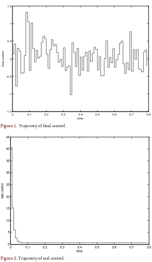
[image:9.595.202.537.87.451.2]

The trajectories of final control and real control are shown in Figure 1 and

Figure 2, respectively. The final control takes into the consideration of noise sequence during the calculation, while the real control is free from the noise

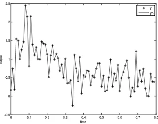
disturbance. Figure 3 shows the trajectories of final output and real output. It

can be seen that the final output tracks closely to the real output. Figure 4 shows the trajectories of final state and real state, where they are statistically identical.

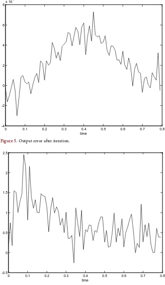
Figure 5 and Figure 6 show, respectively, the output errors after and before ite-rations. The accuracy of the model output is increased due on the decrease of the output error.

Table 1. Simulation result.

Number of Iterations Initial Cost Final Cost Original Cost SSE

(10)

[image:10.595.215.530.62.602.2] [image:10.595.218.529.68.328.2]

Figure 1. Trajectory of final control.

Figure 2. Trajectory of real control.

5. Concluding Remarks

A computational algorithm, which is equipped with the efficient matching scheme, was discussed in this paper. The linear model-based optimal control problem, which is simplified from the discrete time nonlinear stochastic optimal control problem, was solved iteratively. During the calculation procedure, the model used was reformulated into the input-output equations. Then, the least squares optimization problem was introduced. By satisfying the first order neces-sary condition, the normal equation was solved such that the least squares

0 0.1 0.2 0.3 0.4 0.5 0.6 0.7 0.8

-1.5 -1 -0.5 0 0.5 1 1.5

time

fi

nal

c

ont

rol

0 0.1 0.2 0.3 0.4 0.5 0.6 0.7 0.8

0 5 10 15 20 25 30 35 40 45

time

real

c

ont

(11)

[image:11.595.213.534.67.319.2] [image:11.595.213.534.335.602.2]

Figure 3. Trajectories of final output (−) and real output (∗).

Figure 4. Trajectories of final state (−) and real state (+).

recursion formula could be established. In this way, the control policy could be updated iteratively. As a result of this, the sum squares of the output errors was minimized, which indicates the equivalent of the model output to the real out-put. For illustration, an example of the direct current and alternating current converter model was studied. The result obtained showed the accuracy of the algorithm proposed. In conclusion, the efficiency of the algorithm proposed was highly presented.

0 0.1 0.2 0.3 0.4 0.5 0.6 0.7 0.8

-0.5 0 0.5 1 1.5 2 2.5

time

out

put

y yb

0 0.1 0.2 0.3 0.4 0.5 0.6 0.7 0.8

0 0.5 1 1.5 2 2.5 3 3.5

time

s

ta

te

(12)

[image:12.595.206.538.74.645.2]

Figure 5. Output error after iteration.

Figure 6. Output error before iteration.

Acknowledgements

The authors would like to thanks the Universiti Tun Hussein Onn Malaysia (UTHM) for financial supporting to this study under Incentive Grant Scheme for Publication (IGSP) VOT. U417. The second author was supported by the 0 0.1 0.2 0.3 0.4 0.5 0.6 0.7 0.8 -4

-2 0 2 4 6 8x 10

-7

time

0 0.1 0.2 0.3 0.4 0.5 0.6 0.7 0.8 -0.5

0 0.5 1 1.5 2 2.5

(13)

NSF (11501053) of China and the fund (15C0026) of the Education Department of Hunan Province.

References

[1] Ahmed, N.U. (1973) Optimal Control of Stochastic Dynamical Systems. Informa-tion and Control, 22, 13-30. https://doi.org/10.1016/S0019-9958(73)90458-0 [2] Ahmed, N.U. and Teo, K.L. (1974) Optimal Feedback Control for a Class of

Sto-chastic Systems. International Journal of Systems Science, 5, 357-365. https://doi.org/10.1080/00207727408920104

[3] Kliemann, W. (1983) Qualitative Theory of Stochastic Dynamical Systems—Appli- cations to Life Sciences. Bulletin of Mathematical Biology, 45, 483-506.

[4] Adomian, G. (1985) Nonlinear Stochastic Dynamical Systems in Physical Problems,

Journal of Mathematical Analysis and Applications, 111, 105-113. https://doi.org/10.1016/0022-247X(85)90203-3

[5] Li, X., Blount, P.L., Vaughan, T.L. and Reid, B.J. (2011) Application of Biomarkers in Cancer Risk Management: Evaluation from Stochastic Clonal Evolutionary and Dynamic System Optimization Points of View. PLOS Computational Biology, 7, Article ID: e1001087. https://doi.org/10.1371/journal.pcbi.1001087

[6] Lopez, R.H., Ritto, T.G., Sampaio, R. and de Cursi, J.E.S. (2014) Optimization of a Stochastic Dynamical System. Journal of the Brazilian Society of Mechanical Sci-ences and Engineering, 36, 257-264. https://doi.org/10.1007/s40430-013-0067-1 [7] Lozovanu, D. and Pickl, S. (2014) Optimization of Stochastic Discrete Systems and

Control on Complex Networks: Computational Networks, Volume 12 of Advances in Computational Management Science. Springer, Cham Heidelberg, Switzerland. [8] Mellodge, P. (2015) A Practical Approach to Dynamical Systems for Engineers.

Woodhead Publishing, Swaston, Cambridge, UK.

[9] Craine, R. and Havenner, A. (1977) A Stochastic Optimal Control Technique for Models with Estimated Coefficients. Econometrica, 45, 1013-1021.

https://doi.org/10.2307/1912689

[10] Teo, K.L. Goh, C.J. and Wong, K.H. (1991) A Unified Computational Approach to Optimal Control Problems. Longman Scientific and Technical, New York.

[11] Zhang, K., Yang, X.Q., Wang, S. and Teo, K.L. (2010) Numerical Performance of Penalty Method for American Option Pricing. Optimization Methods and Software, 25, 737-752. https://doi.org/10.1080/10556780903051930

[12] Rawlik, K., Toussaint, M. and Vijayakumar, S. (2012) On Stochastic Optimal Con-trol and Reinforcement Learning by Approximate Inference. Proceeding of 2012

Robotics: Science and Systems Conference, Sydney, 9-13 July 2012, 3052-3056. [13] Kek, S.L., Mohd Ismail, A.A. and Teo, K.L. (2015) A Gradient Algorithm for

Op-timal Control Problems with Model-Reality Differences. Numerical Algebra, Con-trol and Optimization, 5, 252-266.

[14] Socha, L. (2000) Application of Statistical Linearization Techniques to Design of Quasi-Optimal Active Control of Nonlinear Systems. Journal of Theoretical and Applied Mechanics, 38, 591-605.

[15] Li, W. and Todorov, E. (2007) Iterative Linearization Methods for Approximately optimal Control and Estimation of Nonlinear Stochastic System. International Journal of Control, 80, 1439-1453. https://doi.org/10.1080/00207170701364913 [16] Zitouni, F. and Lefebvre, M. (2014) Linearization of a Matrix Riccati Equation

(14)

Equa-tions, 2014, Article ID: 741390. https://doi.org/10.1155/2014/741390

[17] Hernandez-Gonzalez, M. and Basin, M.V. (2014) Discrete-Time Optimal Control for Stochastic Nonlinear Polynomial Systems. International Journal of General Sys-tems, 43, 359-371. https://doi.org/10.1080/03081079.2014.892256

[18] Kek, S.L., Teo, K.L. and Mohd Ismail, A.A (2010) An Integrated Optimal Control Algorithm for Discrete-Time Nonlinear Stochastic System. International Journal of Control, 83, 2536-2545. https://doi.org/10.1080/00207179.2010.531766

[19] Kek, S.L., Teo, K.L. and Mohd Ismail, A.A. (2012) Filtering Solution of Nonlinear Stochastic Optimal Control Problem in Discrete-Time with Model-Reality Differ-ences. Numerical Algebra, Control and Optimization, 2, 207-222.

https://doi.org/10.3934/naco.2012.2.207

[20] Bryson, A. and Ho, Y.C. (1975) Applied Optimal Control: Optimization, Estima-tion, and Control. Taylor & Francis, Abingdon.

[21] Lewis, F.L., Vrabie, D.L. and Syrmos, V.L. (2012) Optimal Control. 3rd Edition, John Wiley & Sons, Hoboken. https://doi.org/10.1002/9781118122631

[22] Kirk, D.E. (2004) Optimal Control Theory: An Introduction. Dover Publication Inc., Mineola.

[23] Verhaegen, M. and Verdult, V. (2007) Filtering and System Identification: A Least Squares Approach. Cambridge University Press, Cambridge.

https://doi.org/10.1017/CBO9780511618888

[24] Minoux, M. (1986) Mathematical Programming: Theory and Algorithms. John Wi-ley & Sons, Paris.

[25] Chong, K.P. and Zak, S.H. (2013) An Introduction to Optimization. 4th Edition, John Wiley & Sons, Hoboken.

[26] Poursafar, N., Taghirad, H.D. and Haeri, M. (2010) Model Predictive Control of Nonlinear Discrete Time Systems: A Linear Matrix Inequality Approach. IET Con-trol Theory and Applications, 4, 1922-1932.

https://doi.org/10.1049/iet-cta.2009.0650

[27] Haeri, M. (2004) Improved EDMC for the Processes with High Variations and/or Sign Changes in Steady-State Gain. COMPEL, 23, 361-380.

https://doi.org/10.1108/03321640410510541

[28] Passino, K.M. (1989) Disturbance Rejection in Nonlinear Systems: Example. IEE Proceedings D, 136, 317-323. https://doi.org/10.1049/ip-d.1989.0042

(15)

Submit or recommend next manuscript to SCIRP and we will provide best service for you:

Accepting pre-submission inquiries through Email, Facebook, LinkedIn, Twitter, etc. A wide selection of journals (inclusive of 9 subjects, more than 200 journals)

Providing 24-hour high-quality service User-friendly online submission system Fair and swift peer-review system

Efficient typesetting and proofreading procedure

Display of the result of downloads and visits, as well as the number of cited articles Maximum dissemination of your research work