Munich Personal RePEc Archive
Evaluating density forecasts: a comment
Tsyplakov, Alexander
Novosibirsk State University, Economics Department
30 May 2011
Online at
https://mpra.ub.uni-muenchen.de/32728/
Evaluating Density Forecasts: A Comment
Alexander Tsyplakov
Department of Economics, Novosibirsk State University
August 10, 2011
This is a comment on Mitchell and Wallis(2011) which in turn is a critical reaction toGneiting et al.(2007). The comment discusses the notion of forecast calibration, the advantage of using scoring rules, the “sharpness” principle and a general approach to testing calibration. The aim is to show how a more general and explicitly stated framework can provide further insights into the theory and practice of of probabilistic forecasting.
1
What is “forecast calibration”?
BothGneiting et al.(2007) (hereafter GBR) andMitchell and Wallis(2011) (hereafter MW) examine various important aspects of calibration, but they do not propose a consistent framework and do not give sufficiently universal definitions of “calibration” and the “ideal forecast”. This results in vague argumentation which can lead to confusion. So I start by clearing up the notion of calibration.
The general idea is that a well-calibrated probabilistic forecast must coincide with a suitable con-ditional distribution. The classical definition of calibration for dichotomous 0/1 outcomes requires that among the cases in which a forecast places probability π on the eventX =1 this event must be observed with probabilityπ: P(X =1|π) =π.1 In other words, predicted frequencies must coincide with actual frequencies conditionally on the information contained in the forecast itself. More gener-ally, letF be a probabilistic forecast ofX stated in the form of a cumulative distribution function. It is calibrated if
F(x) =G(x|F),
where G(x|F) is the conditional cumulative distribution function of X given F. I call this type of forecast calibrationauto-calibration.
Now suppose that forecasting is based on some available informationΩ. Then F is a function of
Ω: F =F(·;Ω). Conditioning onΩ allows to strengthen the definition of calibration. The forecast
F =F(·;Ω)iscalibrated with respect toΩif2
F(x) =G(x|Ω).
Such a forecast can be calledthe idealone (of all the forecasts based onΩ).
1E.g. Lichtenstein et al. (1982), p. 307: “Formally, a judge is calibrated if, over the long run, for all propositions
assigned a given probability, the proportion true equals the probability assigned.”
2A formal variant of this definition was proposed independently inGneiting and Ranjan(2011). It is also similar to the
Obviously, if a forecast is calibrated with respect toΩthen it is auto-calibrated while the converse is not true in general. The conditional cumulative distribution functionG(x|Ω)need not coincide with
G(x|F), because a non-ideal forecast utilize available information only partially.
Note that these definitions of calibration are made in terms of theoretical moments. GBR give their definitions of calibration in terms of empirical moments (for a potentially infinite sequence of forecasts).
2
Can independence and uniformity of PIT values be called
com-plete calibration?
One point of MW’s criticism is that GBR are concerned with forecasting of white noise instead of more relevant forecasting of dependent time series. However, what is really important is that GBR do not pay due attention to the conditional nature of calibration.3 MW define “complete calibration” as independence and uniformity of the probability integral transform (PIT) values of a time series. In-deed, it is very true that the available history of a time series (including the PIT values) is an important information for judging calibration of forecasts of this series, but in general this view is unnecessarily narrow. The notion of forecast calibration is not about time series properties, it is about conditioning on forecasting information.
We first need to connect the definition of calibration given above with PIT. If the conditional dis-tribution ofX givenΩis absolutely continuous then a probabilistic forecastF =F(·;Ω)is calibrated with respect toΩif and only if
P|Ω∼U[0,1],
whereP=F(X|Ω)is PIT ofX based on the forecastF.
Now consider a sequenceFt(x)of probabilistic forecasts of a univariate time series Xt based on
its history Ωt−1 =X1, . . . ,Xt−1, t =1,2, . . .. (For t =1 the forecast is unconditional). Define the
corresponding PIT values as follows:
Pt=Ft(Xt).
This provides for eacht a one-to-one transformation betweenP1, . . . ,Pt andΩt=X1, . . . ,Xt whenever
all the distributions are absolutely continuous. The series of forecasts is well-calibrated if and only if
Pt|Ωt−1∼U[0,1]
or, equivalently,
Pt|P1, . . . ,Pt−1∼U[0,1].
MW concentrate on an equivalent property: the series of forecasts is well-calibrated if and only if allPtare distributed asU[0,1]and are jointly independent.4The problem with the PIT-based definition
is that it is insufficiently generic; it does not generalize to other forecasting situations. Using MW’s words, it is important “to pay attention to the information set on which a forecast is based, its content and its timing”.
For example, independence and uniformity of a sequence of PIT values is not sufficient for cal-ibration in the case when forecasts are based on information other than the history of Xt itself. In
3Clements and Taylor(2003), p. 446: “Evaluating probability forecasts by calibration ignores the conditional aspect”. 4Under assumption of calibration with respect to the past history what we have here is the Rosenblatt’s transformation
particular, consider predictingXt fromX1, . . . ,Xt−1 and the history of some other seriesZ1, . . . ,Zt−1.
Then calibration with respect toΩt−1=X1, . . . ,Xt−1,Z1, . . . ,Zt−1is equivalent to
Pt|Ωt−1∼U[0,1],
where Pt =Ft(Xt). For a sequence of forecasts Ft these conditions imply uniformity and
indepen-dence ofPt, but in general uniformity and independence ofPt is a weaker condition. The fact is fully
recognized by MW, but they do not adjust their definition of “complete calibration” accordingly. Another illustration of insufficiency of independence and uniformity of PIT values is the case of the unfocused forecast in the AR(2) example below. In that example forecasting information set includes not only the previous history of the series, but also random noise. Therefore there is no one-to-one correspondence between the previous history and the previous PIT values.
Further, independence of PIT values is not necessary for calibration in a situation of multi-step forecasting. An h-step-ahead forecast of Xt would be based only on X1, . . .Xt−h and the PIT series
corresponding to the ideal forecast would in general be dependent.
3
Testing vs. scoring rules
Suppose that we need to choose between several probabilistic forecasts. When can we state that one forecast is better than another? This is a situation of decision making under risk. Let u(x,a) be a utility function depending on an outcomexand an actiona. Supposea(F)is the best action given a probabilistic forecastF, that is,
a(F)∈arg max
a E[u(X,a)]forX∼F.
One can say thatF1is (non-strictly) better thanF2if it provides at least as large expected utility:
Eu(X,a(F1))≥Eu(X,a(F2)).
This is closely connected with the notion of a proper scoring rule (seeGneiting and Raftery(2007) for a comprehensive review). Define a scoring ruleSas the utility of outcomexunder actiona(F):
S(F,x) =u(x,a(F)).
This utility-based scoring rule would be a proper one since
S(F1,F1) =E[u(X,a(F1)]≥E[u(X,a(F2)] =S(F2,F1) forX∼F1.
Here
S(F2,F1) =E[S(F2,X)] forX ∼F1
is the expected score of forecastF2under the assumption thatX is distributed asF1.
MW argue that non-ideal forecasts can be distinguished from the ideal one by means of testing forecasting models against each other by equal predictive accuracy tests. However, proper scoring rules are no less suitable for the task of detecting the ideal forecast. It can be shown that the well-calibrated forecast is characterized by the maximal expected score for any proper scoring rule.5 In-deed, suppose thatG=G(·|Ω)is such a forecast andFis some other forecast based onΩ. Then
E[S(G,X)|Ω] =S(G,G)≥S(F,G) =E[S(F,X)|Ω]
and
E[S(G,X)]≥E[S(F,X)].
Moreover, under appropriate additional conditions the inequality is strict here if the scoring rule Sis strictly proper. This gives a reason for calling a forecast coinciding with the conditional distribution
G(·|Ω)ideal.
The usefulness of using scoring rules for detecting the ideal forecast is illustrated by Table IV in MW’s paper. They use the logarithmic scoring ruleS(F,x) =logf(x), where f(x) =F′(x)is the prob-ability density function corresponding to the c.d.f. F. The logarithmic rule is known to be (strictly) proper. See also Table 5 in GBR’s paper which compare the average values of the logarithmic score and the continuous ranked probability score (another useful strictly proper scoring rule) of competing forecasts.
Scoring rules are straightforward and easy to deal with. Testing of one forecasting method against another is a less trivial operation while rarely providing much beyond the comparison of average scores. (An example of an understandable use is testing whether the average score of the best method is significantly greater than average scores of rival methods).
Of course, statistical testing is not something redundant in the context of probabilistic forecasting. Most important, various kinds of diagnostic tests can help to develop a forecasting method which is well enough calibrated by showing directions in which methods can be improved. However, discover-ing mis-calibration by diagnostic testdiscover-ing is not always a straightforward task. The followdiscover-ing example is somewhat artificial and is not related to real forecasting problems, but it is suggestive.
Consider a series Xt ∼N(0,1), t =1,2, . . .. To obtainXt fromXt−1 (1) transform Xt toU[0,1],
(2) transformU[0,1]toU[0,1]by a highly nonlinear “tangling” transformation, (3) transformU[0,1]
back to N(0,1), and finally (4) add an independent normal error and scale to unit variance. For example,
µt=Φ−1({K|2Φ(Xt−1)−1|})
p 1−λ,
Xt|X1, . . . ,Xt−1∼N(µt,λ).
HereΦ(·)is the standard normal c.d.f.,{·}is the fractional part function,Kis a large enough integer andλ ∈(0,1). One can see thatXt is a white noise series and is exactly distributed asN(0,1)for each
twheneverX1∼N(0,1)(though it is dependent and thus could not be strictly called a Gaussian white
noise series). For large values of K ordinary PIT-based tests would not detect any dependence. Con-sequently, on the basis of PIT one would chooseN(0,1)as a good forecasting distribution. However,
N(µt,λ)is a dramatically better forecasting distribution for a smallλ.
It can be concluded from the example that sometimes the direction of mis-calibration is not ob-vious. Popular PIT-based diagnostic tests can fail to detect departures from perfect calibration. At the same time comparison of forecasts by their average scores with proper scoring rules is feasible
5Diebold et al.(1998), p. 866: “. . . If a forecast coincides with the true data generating process, then it will be preferred
and works as expected irrespective of the kind of mis-calibration. (A reservation, however, should be made here. If there exists an alternative forecasting method then it can be utilized for the task of testing calibration. Such a test is discussed below.)
Actually MW’s paper is not an exception in its attention to statistical testing of forecasting models. A “test-test-test” bias is typical for econometric forecasting literature in general. Cf. Corradi and Swanson (2006) which is a survey of density forecast evaluation almost entirely devoted to various test procedures.
4
Maximizing sharpness subject to calibration
MW are critical of the conjecture that the problem of finding a good forecast can be viewed as the problem of maximizing sharpness subject to calibration which was stated by GBR. However, it can be shown that the conjecture is actually true provided that a vague “calibration” notion is replaced by auto-calibration introduced above.
IfF is an auto-calibrated forecast (calibrated with respect to itself), that is, F =G(·|F)andS is some scoring rule then
E[S(F,X)|F] =S(F,F).
Taking unconditional expectations of both sides gives
E[S(F,X)] =E[S(F,F)].
For a proper scoring ruleS(F,F)can be viewed as a measure of sharpness6of a probabilistic forecast
F. Hence the expected score for an auto-calibrated forecast equals its expected sharpness. This means that auto-calibrated forecasts can be compared on the basis of the levels of their expected sharpness. The ideal forecast is the sharpest of all auto-calibrated forecasts, because it is characterized by the maximal expected score.
This fact is seen from the classical partitioning of the Brier score for dichotomous outcomes into the sum of sharpness and calibration (“validity”) terms developed in Sanders (1963). For an calibrated forecast the calibration term is zero. Thus, maximizing the expected sharpness among auto-calibrated forecasts is equivalent to maximizing the expected score of a proper scoring rule. Bröcker
(2009) extended the decomposition to the case of an arbitrary discrete distribution and an arbitrary proper scoring rule. It can further be shown that the same decomposition holds even more generally and applies also to continuous distributions.
Given some proper scoring ruleSdefine the divergence7between distributionsF1andF2as
d(F2,F1) =S(F1,F1)−S(F2,F1)
and denote GF =G(·|F). Then for the expected score we have E[S(F,X)] =E[E[S(F,X)|F]] =
E[S(F,GF)]which can be decomposed as follows:
E[S(F,X)] =E[S(GF,GF)]−E[d(F,GF)].
6For a proper scoring ruleS(F,F)is a convex function ofF. Thus, according toDeGroot(1962) a concave function
−S(F,F)can be viewed as a measure of uncertainty of a probability distributionF. For the logarithmic scoring rule
−S(F,F)is the familiar Shannon’s entropy measure.
7The divergenced(F
2,F1)is non-negative as long asSis proper and it is zero when the two distributions coincide. For
The first term can be interpreted as the expected sharpness ofGF, which is the “recalibrated” version of forecastF, while the second term relates to the divergence betweenFandGF (that is, it is a measure
of mis-calibration ofF with respect to information contained in itself).
Although the sharpness conjecture proves to be correct, MW are right in pointing out that the cri-terion of sharpness per se seems somewhat excessive. First, obviously a proper scoring rule already combines sharpness and calibration in a balanced manner. Second, the principle of maximizing sharp-ness subject to calibration is difficult to apply in practice, because achieving perfect auto-calibration of a forecast can prove to be very difficult. However, the sharpness principle provides a useful insight into the essence of probabilistic forecasting.
5
A broader approach to calibration testing
MW rightly note that calibration can be evaluated by testing orthogonality conditions analogous to those known from the theory of point forecasting. It is important that their idea can be further gener-alized, which allows to design various kinds of diagnostic tests for forecast calibration. Many of the tests and criteria of calibration/efficiency developed in the literature can be shown to fall within this approach.
Consider a functionr=r(x,F)of an outcomexand a c.d.f.F. Define
ρ=ρ(F) =E[r(X,F)] forX∼F.
Auto-calibration of a probabilistic forecastF is equivalent to
E[(r(X,F)−ρ(F))] =0
for anyr. That is,ρmust be an unbiased point forecast forr. The perfect calibration ofFwith respect toΩis a stronger property and requires conditional unbiasedness:
E[(r(X,F)−ρ(F))|Ω] =0.
This conditional unbiasedness is equivalent to the following unconditional orthogonality:
E[(r(X,F)−ρ(F))q(Ω)] =0
for anyqwhich is a function of available informationΩ. That is,ρmust be an unbiased point forecast forrand the forecast error must be uncorrelated with any functionqof the available informationΩ.
Example 1. For absolutely continuous case when
r=1{F(x)≤p}, ρ=p (1)
for p∈[0,1], we obtain an extended version of the “probabilistic calibration” of GBR. The orthogo-nality condition E[(r−p)q] =0 for each p∈[0,1]and any function q=q(Ω)is another equivalent characterization of the perfect calibration with respect to Ω. Note that unlike the formulation by GBR this one does not make direct use of the ideal forecastG(·;Ω)and thus is more suitable for the construction of tests.
Example 2. Similarly, the “marginal calibration” of GBR corresponds to
Example 3. “Tests of efficiency” proposed by MW are also a special case of this approach with
r=Φ−1(F(x))andρ =0.
More generally, consider a function m=m(x,Ω) depending on an outcome x and forecasting informationΩ. Define
µ =µ(Ω) =E[m(X,Ω)] forX∼F =F(·;Ω).
Calibration ofF with respect toΩis equivalent to the following moment condition:
E[(m(X,Ω)−µ(Ω))] =0
for anym.
Example 4. One more example parallels equal predictive accuracy tests based on the difference of the logarithmic scores (or Kullback–Leibler information criterion, KLIC) discussed by MW (see
Amisano and Giacomini (2007)). The idea is to test calibration of one forecasting method against another one. Suppose that we want to test whetherF1=F1(·;Ω)is well-calibrated and F2=F2(·;Ω)
is an alternative forecast. Let m=S(F2,X)−S(F1,X)for some proper scoring rule S. For a forecast
F1which is calibrated with respect toΩ
µ =E[m|Ω] =S(F2,F1)−S(F1,F1).
So we can test calibration ofF1by testing that
E[(S(F2,X)−S(F1,X))−(S(F2,F1)−S(F1,F1))] =0. (2)
Below we call this moment condition relative forecast calibration (RFC). A test based on it would have power against an alternative thatF2is calibrated with respect toΩ, because then
E[m−µ] =E[(S(F2,F2)−S(F1,F2)] +E[(S(F1,F1)−S(F2,F1)]>0,
if the scoring rule is strictly proper.
For the case of the logarithmic score and two normal forecasting distributions, N(α1,σ12) and
N(α2,σ22), the moment condition reduces to
Eh 1 2σ22 σ
2
1+ (α1−α2)2−(X−α2)2
− 1
2σ12 σ
2
1−(X−α1)2
i
=0.
A pair of reciprocal RFC-based tests (F1 againstF2andF2 againstF1) can help to judge possible
gains from combining two forecasts.
6
Example: Forecasting an autoregressive process
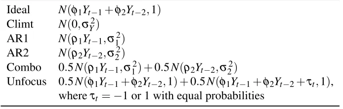
To illustrate the ideas I first adopt the simulation example from MW’s paper which relates to forecast-ing of AR(2) seriesYt =φ1Yt−1+φ2Yt−2+εt with independent Gaussian disturbancesεt ∼N(0,1).
Table1lists six forecasting models to be compared. The actual data-generating process is represented by the ideal forecast. In this example there is no need to estimate parameters as they are known. I consider only the Case (2) withφ1=0.15,φ2=0.2. The length of the series isT =150 if not specified
otherwise.
Table 1: Definition of six forecasts of AR(2)
Ideal N(φ1Yt−1+φ2Yt−2,1)
Climt N(0,σY2)
AR1 N(ρ1Yt−1,σ12)
AR2 N(ρ2Yt−2,σ22)
Combo 0.5N(ρ1Yt−1,σ12) +0.5N(ρ2Yt−2,σ22)
Unfocus 0.5N(φ1Yt−1+φ2Yt−2,1) +0.5N(φ1Yt−1+φ2Yt−2+τt,1),
whereτt=−1 or 1 with equal probabilities
Note: ρ1=φ1/(1−φ2), ρ2=φ1ρ1+φ2, σY2=1/(1−φ1ρ1−φ2ρ2), σ12=
(1−ρ2
1)σY2,σ22= (1−ρ22)σY2.
narrowing of the opportunities for calibration testing. More general moment conditions can be fruit-fully utilized. Second, I want to illustrate separation of model selection from diagnostic testing as opposed to mixing them in pairwise equal predictive ability tests.
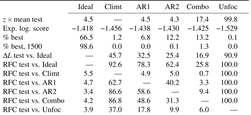
Consider the unfocused forecast. Unconditionally it is probabilistically calibrated which leads to uniformity of PIT (cf. Table II of MW). Also the PIT series are serially independent (cf. Table III of MW). However, it is not auto-calibrated, which can be easily detected using a test of orthogonality between the inverse normal transformation of PITzt =Φ−1(Ft(yt))(which should be unconditionally
distributed asN(0,1)under auto-calibration) and the mean of the forecasting distribution. It is labeled “z×mean test” in Table2. For an auto-calibrated forecast we haveE[mean(Ft)zt] =0. The table shows
that this condition is rejected in almost 100% of experiments in the case of the unfocused forecast. Here and below I use the usual t-ratios based on heteroskedasticity and autocorrelation consistent (HAC) standard errors for testing moment conditions. The results confirms also that the combined forecast (“Combo”) which is a weighted combination of AR1 and AR2 is not auto-calibrated (although the rejection rate is not very large), while for other forecasts there are no signs of mis-calibration (indeed, ideal, AR1 and AR2 forecasts are all auto-calibrated).
The row labeled “% best” shows the percent of experiments in which the corresponding model had the highest average logarithmic score. The ideal forecast was the best with probability of about 2/3. This moderately large value is explained by small values of the two autoregression coefficients (φ1=0.15, φ2=0.2), which makes the true data generating process rather close to AR1, AR2 and
Combo alternatives in terms of the expected logarithmic score for relatively short series (T =150). WithT =1500 the ideal forecast dominates the other ones (see row labeled “% best, 1500”). One can see that the average score is a sensible criterion for model selection which behaves in a predictable way. Testing is not really needed for the task of model selection. Of course, a test of whether the chosen model has significantly higher average score than the competitors in the spirit ofWhite(2000) orHansen(2005) can be useful.
To test calibration of the forecasting models against each other I employ a relative forecast cali-bration test based on the RFC property discussed above. The test is designed as one-sided to increase its power, because the test statistic is expected to be positive in situations when the alternative forecast can potentially be used to improve the forecast tested for calibration. Notable are the results of AR1 vs. AR2 and AR2 vs. AR1. The tests would frequently suggest the usefulness of combining the two mod-els. The test against the ideal forecast can be seen to have high power. It can be compared to the equal predictive ability test based on the difference of the attained average scores∆Lt=S(Gt,yt)−S(Ft,yt)
[image:9.612.141.488.82.193.2]Table 2: Statistics for six forecasts of AR(2)
Ideal Climt AR1 AR2 Combo Unfoc
z×mean test 4.5 — 4.5 4.3 17.4 99.8
Exp. log. score −1.418 −1.456 −1.438 −1.430 −1.425 −1.529
% best 66.5 1.2 6.8 12.2 13.2 0.1
% best, 1500 98.6 0.0 0.0 0.1 1.3 0.0
∆Ltest vs. Ideal — 45.7 32.5 25.4 16.9 90.9
RFC test vs. Ideal — 92.6 78.3 62.4 25.8 100.0
RFC test vs. Climt 5.5 — 4.9 5.0 0.7 100.0
RFC test vs. AR1 4.7 62.7 — 40.2 3.3 100.0
RFC test vs. AR2 3.4 86.6 58.6 — 9.4 100.0
RFC test vs. Combo 4.2 86.8 48.6 31.3 — 100.0
RFC test vs. Unfoc 3.9 37.0 17.8 9.9 6.0 —
Note: The table is based on 5000 simulations. The figures for the tests are percentages of rejection at 5% asymptotic significance level using the standard normal quantiles. The test statistics are t-ratios with Newey–West HAC standard errors and lag truncation 4. “% best, 1500” corresponds to 10 times longer series (T =1500). The row labeled “Exp. log. score” shows approximate expected logarithmic scores. S(F2,F1)functions for mixtures of
nor-mals needed for RFC statistics are computed by Monte Carlo with 100 simulations.
of identifying non-ideal forecasts.
7
Example: Forecasting a stock index
The second example is intended to show how the proposed framework can be utilized for the task of evaluating forecasts of real-world time series. The data are daily close levels of Russian stock market index (RTSI) and span the period from 1995-09-01 to 2011-06-08. The RTSI series is brought to stationarity by computing its growth rates in percent yt = (logRT SIt−logRT SIt−1)×100. This
provides a series of 3,928 observations. The forecasted variable is the growth rate 10 periods ahead. Thus, at timet a forecast of yt+1+· · ·+yt+10= (logRT SIt+10−logRT SIt)×100 is obtained. (The
ten-period horizon corresponds roughly to two weeks of physical time.) The following forecasts are considered.8
1. The historical forecast based on the full history (“Hi-full”) uses previously observed 10-period growth rates. The historical observations are resampled to obtain a sample of size 1000.
2. “Hi-200” is also a historical forecast, but uses only a rolling span of the 200 most recent obser-vations and does not use resampling.
3. “ExpSm” forecast is based on exponential smoothing for volatility σ2
t =δy2t−1+ (1−δ)σt2−1
with the decay factorδ=0.95. The forecasting distribution is given byN(0,10ht)and is derived from an assumption of a Gaussian random walk with the varianceht. The recursion for volatility
starts from the sample variance of the first 200 observations.
8The RTSI series exhibits significant first-order serial correlation, but its impact on 10-period-ahead forecasts is small
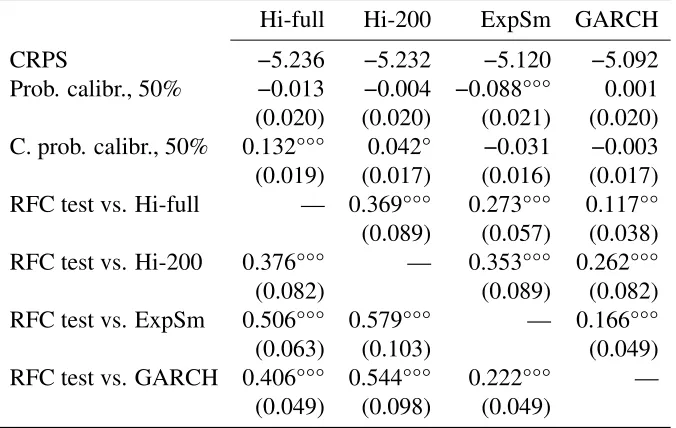
Table 3: Forecasts of RTSI
Hi-full Hi-200 ExpSm GARCH
CRPS −5.236 −5.232 −5.120 −5.092
Prob. calibr., 50% −0.013 −0.004 −0.088°°° 0.001
(0.020) (0.020) (0.021) (0.020) C. prob. calibr., 50% 0.132°°° 0.042° −0.031 −0.003 (0.019) (0.017) (0.016) (0.017)
RFC test vs. Hi-full — 0.369°°° 0.273°°° 0.117°°
(0.089) (0.057) (0.038)
RFC test vs. Hi-200 0.376°°° — 0.353°°° 0.262°°°
(0.082) (0.089) (0.082)
RFC test vs. ExpSm 0.506°°° 0.579°°° — 0.166°°°
(0.063) (0.103) (0.049)
RFC test vs. GARCH 0.406°°° 0.544°°° 0.222°°° —
(0.049) (0.098) (0.049)
Note: Newey–West HAC standard errors with lag truncation 10 are shown in brackets. Statis-tical significance at 5% (1%, 0.1%) level is shown by°(°°,°°°). RFC tests areCRPS-based.
4. GARCH forecast is based on the standard GARCH(1,1)-t model (GARCH with t distribution) with non-zero mean. The model is estimated recursively by the maximum likelihood method. The forecasting distribution is represented by a sample of 1000 simulated future trajectories.
All the forecasts are produced recursively for the forecasting period staring from the 200-th ob-servation. They are compared by their observed averages of the continuous ranked probability score (CRPS). CRPS can be defined as
S(Ft,yt) =
1
2E|Y−Y
′| −
E|Y−yt|.
for a pair of independentY,Y′from the forecasting distributionFt and can be calculated inO(NlogN)
operations needed for sorting ifFt is represented by a sample of sizeN (Gneiting and Raftery(2007)).
One advantage of the CRPS over the logarithmic scoring rule is that it allows a forecast of a continuous random variable to be a discrete distribution. This scoring rule is also appealing, because it can be viewed as a generalization of the absolute distance loss which is a popular criterion for evaluation of point forecast.
The following statistics are summarized in Table3.
1. “CRPS” is the averageCRPS.
2. “Prob. calibr., 50%” is an unconditional probabilistic calibration statistic based on (1) for
p=0.5. This statistic relates to the location as measured by the median of the forecasting distribution.
3. “C. prob. calibr., 50%” is a central unconditional probabilistic calibration statistic with
r=1{F(y)∈[(1−p)/2,(1+p)/2]}, ρ= p
(a) 0 0.2 0.4 0.6 0.8 1 1.2
0 0.2 0.4 0.6 0.8 1
(b) 0 0.2 0.4 0.6 0.8 1 1.2
[image:12.612.154.461.63.160.2]0 0.2 0.4 0.6 0.8 1
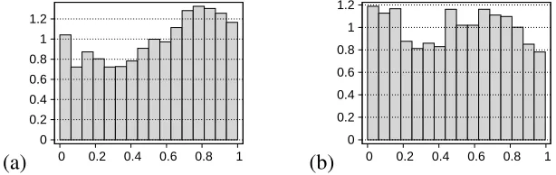
Figure 1: Histograms of PIT values: (a) exponential smoothing; (b) GARCH
4. “RFC vs.hmethodi” is a one-sided RFC test, the same as in previous example, but based on the CRPS.
The selection of the calibration tests is somewhat arbitrary. The proposed framework allows to design many different tests, including other kinds of probabilistic calibration tests. Such tests are formal counterparts of visual inspection of PIT histograms, a method which is frequently employed for evaluation of density forecasts.9
The example pertains to a typical practical situation when none of the compared forecasts can be called “ideal”. All forecasts are not well-calibrated to different degrees (Table3). For example “Hi-full” while having (unconditionally) correct location (see “Prob. calibr., 50%”) notably lack sharpness which is signaled by central probabilistic calibration: the actual values are too seldom found in the tails. “ExpSm” rigidly assumes zero mean which is not corroborated by the observed data and the probabilistic calibration test with p=50% indicates a negative bias accordingly; note also the skew of the histogram in Figure1(a).
In general “GARCH” looks almost like a calibrated forecast if calibration is judged on the basis of ordinary PIT-based criteria. The histogram of PIT values at Figure1(b) is not perfectly flat, but its unevenness is not very serious as confirmed by the two probabilistic calibration tests from Table 3. Also there are no serious signs of autocorrelation after lag 10 in both zt = Φ−1(Ft(yt)) and zt′ =
Φ−1(|2Ft(yt)−1|) (calculated from the “folded” PIT values |2Ft(yt)−1| and designed to capture
unaccounted volatility clustering). For example, the 11-th autocorrelation coefficient is 0.071 for zt
and−0.033 forz′t while asymptotic standard errors are 0.045 and 0.031 respectively.10
GARCH model is the leader in terms of the average CRPS level, followed closely by exponen-tial smoothing. However, all of the methods in pairwise comparisons by means of RFC tests show significant mis-calibration. For example, remarkably, GARCH is not able to encompass exponen-tial smoothing, which can be considered as its “cheaper” substitute. The results show a potenexponen-tial for improving the forecasts by combining them.
8
Conclusions
Probabilistic forecasting steadily gains popularity and the two papers, Mitchell and Wallis (2011),
Gneiting et al. (2007), make important contributions into this process. However, when discussing statistical procedures related to forecast calibration it seems natural to rely on a generic definition. My
9The problem with the histograms is that they can be potentially deceptive without error bands which are robust to
heteroskedasticity and autocorrelation.
10The Bartlett’s approximation for the variance ofr
11is used which assumes no autocorrelation after lag 10 and is given
comment provides such a definition of calibration and delineates a general framework for calibration testing. The framework can facilitate construction of various diagnostic tests. An example of an interesting new test derived from these principles is a relative forecast calibration (RFC) test.
The current discussion accentuates several noteworthy points related to probabilistic forecasting.
• Uniformity and independence of PIT values as a condition of forecast calibration relates to an unreasonably narrow class of forecasting situations when forecasts of a time series are based on its own full history.
• When evaluating forecasts it is important to remember about possible goals of forecasting. Maximizing expected score corresponding to some proper scoring rule can be considered as a reduced representation of such goals.
• Statistical testing is not a substitute for using scoring rules when it is needed to select one method from a fixed set of forecasting methods. Consequently, equal predictive ability tests can be redundant in such a situation.
• Some types of mis-calibration cannot be detected by conventional PIT-based tests. In general calibration tests should be based the relevant information set.
• “Maximizing sharpness subject to (auto-)calibration” is a legitimate principle of probabilistic forecasting. However, its usefulness is limited, because in practice it is hard to achieve perfect auto-calibration.
• RFC-type tests can be rather sensitive to mis-calibration, which suggests that this class of tests is a natural replacement for equal predictive ability tests in the task of diagnosing imperfections of forecasting methods.
References
Amisano, G. and Giacomini, R. (2007). Comparing density forecasts via weighted likelihood ratio tests,Journal of Business and Economic Statistics25(2): 177–190.
Bröcker, J. (2009). Reliability, sufficiency, and the decomposition of proper scores,Quarterly Journal of the Royal Meteorological Society135(643): 1512–1519.
Christoffersen, P. F. (1998). Evaluating interval forecasts,International Economic Review39(4): 841– 862.
Clements, M. P. and Taylor, N. (2003). Evaluating interval forecasts of high-frequency financial data,
Journal of Applied Econometrics18(4): 445–456.
Corradi, V. and Swanson, N. R. (2006). Predictive density evaluation, inC. W. J. Granger, G. Elliott and A. Timmermann (eds),Handbook of Economic Forecasting, Vol. 1, North-Holland, Amsterdam, chapter 5, pp. 197–286.
DeGroot, M. H. (1962). Uncertainty, information, and sequential experiments,The Annals of Mathe-matical Statistics33(2): 404–419.
Gneiting, T., Balabdaoui, F. and Raftery, A. E. (2007). Probabilistic forecasts, calibration and sharp-ness,Journal of the Royal Statistical Society: Series B69: 243–268.
Gneiting, T. and Raftery, A. E. (2007). Strictly proper scoring rules, prediction, and estimation,
Journal of the American Statistical Association102: 359–378.
Gneiting, T. and Ranjan, R. (2011). Combining predictive distributions, ArXiv preprint.
arXiv:1106.1638v1 [math.ST].
Granger, C. W. J. and Pesaran, M. H. (2000). A decision-theoretic approach to forecast evaluation,
inW.-S. Chan, W. K. Li and H. Tong (eds),Statistics and Finance: An Interface, Imperial College Press.
Hansen, P. R. (2005). A test for superior predictive ability,Journal of Business & Economic Statistics
23(4): 365–380.
Lichtenstein, S., Fischhoff, B. and Phillips, L. D. (1982). Calibration of probabilities: The state of the art to 1980, in D. Kahneman, P. Slovic and A. Tversky (eds), Judgment under Uncertainty: Heuristics and Biases, Cambridge University Press, Cambridge, UK, pp. 306–334.
Mitchell, J. and Wallis, K. F. (2011). Evaluating density forecasts: Forecast combinations, model mixtures, calibration and sharpness,Journal of Applied Econometrics,n/a: ??–?? forthcoming.
Rosenblatt, M. (1952). Remarks on a multivariate transformation, Annals of Mathematical Statistics
23: 470–472.
Sanders, F. (1963). On subjective probability forecasting,Journal of Applied Meteorology2: 191–201.