Munich Personal RePEc Archive
Privatization of Knowledge: Did the U.S.
Get It Right? (New Version).
Cozzi, Guido and Galli, Silvia
University of Durham, University of Hull
15 January 2011
Privatization of Knowledge: Did the U.S. Get It Right?
Guido Cozzi
yand Silvia Galli
zAbstract
To foster innovation and growth should basic research be publicly or privately funded? This paper studies the impact of the gradual shift in the U.S. patent system towards the patentability and commer-cialization of the basic R&D undertaken by universities. We see this movement as making universities becoming responsive to "market" forces. Prior to 1980, universities undertook research using an exoge-nous stock of researchers that were motivated by "curiosity." After 1980, universities patent their research and behave as private …rms. This move, in a context of two-stage inventions (basic and applied re-search) has an a priori ambiguous e¤ect on innovation and welfare. We build a Schumpeterian model and match it to the data to assess this important turning point. Keywords: R&D and Growth, Sequential Innovation, Basic Research, Patent Laws. JEL Classi…cation: O31, O34, O41.
We thank two anonimous Referees and an Associate Editor for their extremely helpful comments and suggestions. We are also grateful to seminar participants at the University of Bologna, at the University of Rome "La Sapienza", at the University of Louvain la Neuve, at Tilburg University, and at the University of Edinburgh for comments.
yDurham University Business School, room 118, Mill Hill Lane, Durham, DH1 3LB,
United Kingdom, e-mail: [email protected]
zHull University Business School, Economics, Cottingham Road, Hull HU6 7RX,
1
Introduction
Over the last 30 years, U.S. Court decisions switched from the doctrine limiting the patentability of early-stage scienti…c …ndings - lacking in current commercial value - to the conception that also fundamental basic scienti…c discoveries - with no current tradeable application - fall in the general ap-plicability of the patent system.
The year 1980 marked an important turning point in US patentability requirements, as summarized by the following events:
1. the United States Supreme Court’s decision on the Diamondsv. Chakrabarty
case ruled that microorganism produced by genetic engineering could be patented;
2. the Bayh-Dole Act, which facilitated universities in patenting innova-tions.
After the second world war, universities and public laboratories had al-ways been the main performers of basic R&D in the United States and in Europe. Though an important reason for the relatively low private contri-bution to basic R&D is often found in the high degree of uncertainty that this activity involves in terms of future commercial application and success, the legal permission to appropriate the fruits of years of investigations makes a big di¤erence, and marks an important change from the pre-1980 to the post-1980 US innovation system. Hence the 1980’s jurisprudential and ju-ridical reforms opened the way to a ‡ow of private funds into the academia in search of promising research projects, as well as facilitated professors in patenting their own research without incurring in legal obstacles linked to their direct or indirect involvement in the public system.
Jensen and Thursby (2001) studied the more recent licensing practices of 62 US universities. They found that "Over 75 percent of the inventions licensed were no more than a proof of concept (48 percent with no proto-type available) or lab scale protoproto-type (29 percent) at the time of license!". Moreover, most of the inventions licensed were in such an embryonic state of development, that it was di¢cult to estimate their commercial potential and the inventor’s cooperation was required to get a successful commercial development.
the laboratory”, and includes "cell lines, monoclonal antibodies, reagents, animal models, growth factors, combinatorial chemistry libraries, drugs and drug targets, clones and cloning tools... methods, laboratory equipment and machines, databases and computer software". Nearly all research tools be-came patentable in the US, thanks to the juridical innovations that took place in the last 30 years.
The agreement on Trade-Related Aspects of Intellectual Property Rights (TRIPs), article 27, encourages countries to extend patentability to"any in-ventions, whether products or processes, in all …elds of technology, provided that they are new, involve an inventive step and are capable of industrial application", and a footnote follows specifying: "For the purposes of this Ar-ticle, the terms "inventive step" and "capable of industrial application" may be deemed by a Member to be synonymous with the terms "non-obvious" and "useful" respectively." Hence a "useful" research tool should be patentable. Though to ".. make all research activities free of patent infringement would make all research tool patents worthless, and would be contrary to TRIPs",
(Thouret-Lemaitre1, 2006), the adoption of TRIPs by several countries is
still controversial, as strong research exemptions to patent infringement are in place in countries such as Japan2, China3, Belgium4, Germany5, India6,
1Elisabeth Thouret-Lemaitre, Vice President, Head of Patent Operations,
Sano…-Synthelabo, Paris, WIPO Presentation October 11, 2006.
2Japan: art 69 (1): " the e¤ects of the patent right shall not extend to the working of
the patent right for the purposes of experiment or research."
3Article 62 of the Patent Law of the People’s Republic of China: "None of the following
shall be deemed an infringement of a patent right:...5. Use of the patent in question solely for the purposes of scienti…c research and experimentation".
4Where since 2005 the new Article 28(1)(b) of the Belgian Patent Act states that a
patent holder’s claims “do not extend to acts that are committed on and/or with the subject of the patented invention for scienti…c purposes”.
5The German Constitutional Court (2000) stated that patent holders must "accept
such limitations on their rights in view of the development of the state of the art and the public interest". Thus the patent claims become controversial when the commercial interest of the unauthorized use of a patented innovation is not clear.
6Section 47 of the Patent Act states that The patented product or process "may be
Brazil7, Mexico8, and Korea9. Even if the European Directive on
Biotech-nology of 1998 aimed at extending patentability to many research tools, it is still being implemented in contradictory ways, leading to a situation in the middle between the pre- and post-1980 US regime. Statutory research exemptions and compulsory licensing render patent claims much weaker.
We believe that an economic analysis of the US turning point may give good insight to start a scienti…c debate rich of relevant policy implications at least for Europe. This paper, by taking the R&D sequentiality into the Schumpeterian paradigm, investigates the relation between the cumulative uncertainty involved in the two-stages innovation process and the ine¢ciency in the public research system. Our main theoretical contribution is a the-ory of endogenous public ine¢ciency in basic research. Regarding private
research, we share the decomposition of each innovation in two stages of
re-searchanddevelopment with the oligopolistic patent race literature pioneered by Reinganum (1985), Grossman and Shapiro (1986) and (1987), and, more recently, Denicolò (2000). We contribute with several new insights, by adding free entry, endogenous multisector industrial dynamics and general equilib-rium determination of all variables. Our general equilibequilib-rium analysis allows a consistent numerical calibration of our theory to the true US data. The main alternative macroeconomic predecessor is Aghion and Howitt (1996), which identi…ed basic research with horizontal innovation10. Since in the real world
all sectors need basic research not just once, we adopt the complementary view that basic research pervades all sectors, which forces us to substantially
modify the standard multisector framework with vertical innovation11. We
7Article 43 of the Brazilian Industrial Property Law: "The provisions of the preceding
Articles shall not apply:...II. to acts carried out for experimental purposes by unauthorized third parties if related to study or to scienti…c and technological research."
8Article 22 of the Industrial Property Law: "The right conferred by a patent shall
not have any e¤ect against: (I) a third party who, in the private or academic sphere and for non-commercial purposes, engages in scienti…c or technological research activities for purely experimental, testing or teaching purposes, and to that end manifactures or uses a product or a process identical to the one patented".
9Section 96(1) of the Patent Law states: "The e¤ects of the patent right shall not
extend to the following: (i) working of the patented invention for the purpose of research or experiment. . . ".
10Gersbach, Sorger, and Amon (2009) extends this framework, with basic research
po-tentially opening more new sectors than applied research manages to complete. Bramoulle’ and Saint-Paul’s (2010) incorporates a realistic reputation reward system based on cita-tions.
will assume that basic research can be "curiosity driven", but that it could also be motivated by its potentially socially useful applications.
The rest of this paper is organized as follows. Section 2 explains the mod-i…cations in Schumpeterian theory needed to analyse the two-stage innova-tion process stylizing the innovative mechanism in the presence of research tools. It focusses on the most original aspects of the model, leaving the most standard parts to the Appendix 1, in order to facilitate readability. Sec-tion 3 applies this new framework to a stylized pre-1980 US scenario: basic research …ndings are conceived in public institutions and put into the pub-lic domain, triggering patent races by freely entering perfectly competitive private R&D …rms aiming at inventing a better quality product. Section 4 models a stylized post-1980 US scenario, where basic R&D achievements are patented and, afterwards, developed into tradable applications within a com-pletely privatized economy. Free entry patent races only occur in the basic research, whereas as soon as a research tool is discovered it will be developed by its patent holder. Section 5 matches the model to the US data prevailing at the time of the jurisprudence and legislative change. We estimate the relevant technological parameter and we undertake numerical simulations in order to assess if the reform could have enhanced innovation. In Section 6, we test the robustness of our …ndings in an alternative model of privatized basic research, which explicitly includes the debated existence of a "research exemption", which might give birth to reach-through patenting agreements after an infringement suit. Section 7 concludes.
2
The Model
2.1
Overview
Consider an economy with a continuum of di¤erentiated …nal good sectors with corresponding di¤erentiated research and development (R&D) sectors, along the lines of Grossman and Helpman (1991a and b). In each sector there is a instantaneous price competition, which implies - under the usual constant returns to scale assumption - that at every date there will be a monopolist, that coincides with the owner of the patent on the highest quality product
in its industry. Product improvements occur in each consumption good in-dustry, and, within each inin-dustry, …rms are distinguished by the quality of the …nal good they produce. When the state-of-the-art quality product in an industry ! 2[0;1] is jt(!), R&D …rms compete in order to learn how to
produce thejt(!) + 1st quality product. We extend the standard quality
lad-ders model by introducing a two-stage innovation path, so …rst a researcher catches a glimpse of innovation through the jt(!) + 12th inventive half-idea,
and then other researchers engage in a patent race to implement it in the
jt(!) + 1st quality product12. The best real world interpretation of our "half
ideas" are the research tools. So, in each industry, the R&D activity is a two stage process by which, …rst a new idea is invented upstream - a …rst "half-idea" - and then it is used to …nd the way to introduce a higher qual-ity product: in the words of Grossman and Shapiro (1987, p.373), the "two stages may be thought of as research and development, respectively."
As in Grossman and Helpman (1991a and b), time is continuous with an unbounded horizon and there is a continuum of in…nitely-lived households with identical intertemporally additive preferences. Heterogeneous labour, skilled and unskilled, is the only factor of production. Both labour
mar-kets are assumed perfectly competitive. In the …nal good sectors ! 2 [0;1]
monopolistically competitive patent holders of the cutting edge quality good produce di¤erentiated consumption goods by combining skilled and unskilled labour, whereas research …rms employ only skilled labour. To facilitate the exposition, the most standard analytical details of the model can be found in the Appendix 1.
2.2
The Mechanics of R&D, and Preliminary Results
In our economy the whole set of industries f! 2 [0;1]g gets partitioned
into two subsets of industries: at each date t, there are industries ! 2 A0
with (temporarily) no research tool and, therefore, with one quality leader (the …nal product patent holder), no applied research and a mass of basic researchers, and the industries ! 2 A1 = [0;1]n A0, with one research tool
and, therefore, one quality leader and a mass of applied researchers directly
12Of course, half ideas could be as di¢cult to get as are Nobel prizes: see, for example,
challenging the incumbent monopolist. Researchers engage in useful13 basic
R&D only in ! 2 A0 industries, while R&D …rms engage in applied R&D
activity aimed at a …nal product innovation only in A1 industries. When a
quality improvement occurs in an A1 industry, the innovator becomes the
new quality leader and the industry switches from A1 toA0. Similarly, when
a discovery arises in an industry! 2A0 this industry switches toA1. Figure
[image:8.612.171.471.254.386.2]1 illustrates the ‡ow of industries from a condition to the other:
Figure 1 Representation of the economy by ‡ows of industries
Notice that in our multisector two-stage environment with perpetual inno-vation basic R&D alternates with applied R&D in all sectors of the economy. The two setsA0 andA1 change over time, even if the economy will eventually
tend to a steady state. At any instant we can measure the mass of industries without any half-idea as m(A0)2 [0;1], and the mass of industries with an
uncompleted half-idea as m(A1) = 1 m(A0). Clearly, in the steady state
these measures will be constant, as the ‡ows in and out will o¤set each other. However, the endogenous nature of the steady state equilibrium distribution of sectors allows us to study the e¤ects of di¤erent institutional scenarios -patentability regimes, public sector ine¢ciency - on technological dynamics
and aggregate innovation. Let index i = B; A denote basic or applied
re-search. ni(!; t),indicates the mass of skilled labor employed in basic, and,
respectively, applied research in sector ! 2 [0;1] at date t. A researcher’s
13In one of the three economies stylized in this paper, namely the Public Basic Research
scenario, some basic research is undertaken also in A1 industries, but it produces no
Poisson process probability of succeeding in inventing a half-idea, or com-pleting one (i.e. introducing the product innovation), is decreasing in the
aggregate sectorial R&D labor, ni 0. In particular, we specify the
per-unit time Poisson probability intensity to succeed for a basic and an applied research labour unit respectively as
B(!; t) 0nB(!; t) a, !2A0 (1)
A(!; t) 1nA(!; t) a , ! 2A1 (2)
where k >0, k= 0;1, are R&D productivity parameters14 and constant
0< a < 1 is an intra-sectorial congestion parameter, capturing15 the risk of
R&D duplications, knowledge theft and other diseconomies of fragmentation in the R&D. Each Poisson process - with arrival rates described by (1)-(2) - governing the assumed two-stage innovative process is supposed to be independent across researchers and across industries. Hence the total amount of probability per unit time of inventing a basic half idea in a sector ! 2A0
at datetisnB(!; t) B(!; t)and the total amount of probability per unit time
of completing a basic research tool in a sector ! 2A1 isnA(!; t) A(!; t).
Moreover, in all our scenarios, symmetric equilibria exist, allowing us to simplify notation: nB(!; t) nB(t) and nA(!; t) nA(t).
2.2.1 Manufacturing
So far we have assumed an exogenously given aggregate amount of skilled labour, L, employable in the manufacturing and in the R&D sectors; and an
exogenously given aggregate amount of unskilled labour,M, only employable
in manufacturing. Adopting the unskilled wage as the numeraire, we will endogenously determine the skill premium, as summarized by the skilled labour (relative) wage ws.
14Eq.s (1)-(2) are build on the assumption of a stationary population. With increasing
population, it is easy to recast our model, as done in Appendix 1, in terms of Dinopoulos and Segerstrom’s (1999) PEG framework, which captures the di¢culty of improving a good in a way that renders a larger population happier. This eliminates the strong scale e¤ect (Jones 2003) that plagued the early generation endogenous growth models, without leading to "semi-endogenous" growth (Jones 1995, Segerstrom 1998), as consistent with recent empirical evidence (e.g. Madsen, 2008). Despite its semplicity, this assumption is equivalent to eliminating the strong scale e¤ect by means of an R&D "dilution e¤ect" over an increasing range of varieties, as proved by Peretto (1998), Young (1998), Dinopoulos and Thompson (1998) and (1999), and Howitt (1999).
In all our equilibria, the per-capita mass of skilled labour employed in manufacturing sector ! 2 [0;1] at time t, labeled x(!; t), will be constant across sectors and equal to x(!; t) = x(t). In fact, in the Appendix 1 we prove that the manufacturing employment of the skilled labour obeys the following decreasing function of the relative skilled wage ws:
x(!; t) = 1
ws(t) 1
M x(t),
where 0 < < 1 is the skilled labour elasticity of output. Appendix
2 also show that at any date the pro…t ‡ows are constant and equal to
= ( 1) 1
1 M, where >1 is the size of each product quality jump.
Since the total mass of sectors in the economy is normalized to1,x(t)also denotes the aggregate employment of skilled in manufacturing. Hence, these always hold: x(t)ws(t) = Y(t)andM =M wu(t) = (1 )Y(t), whereY(t)
is aggregate …nal good production.
In light of the previous discussion, and dropping time indexes for simplic-ity16, we can express the skilled labor market equilibrium as:
L= 1
ws 1
M +m(A0)nB+m(A1)nA. (3)
Eq. (3) states that, at each date, the aggregate supply of skilled labor, L,
…nds employment in the manufacturing …rms of all [0;1] sectors, x, and in
the R&D laboratories of the A0 sectors,nB, and of the A1 sectors, nA.
3
The Public Basic Research Economy
In this section we assume unpatentable basic scienti…c results, in order to depict a pre-1980 US normative environment. In our model, public R&D is allocated regardless of pro…t opportunities: since researchers get paid regard-less of the pro…tability of their discoveries, their activity is "curiosity driven", and their rewards are not aligned to downstream needs. Hence their e¤orts might, from a social viewpoint, be wrongly targeted. To stylize the partially "un-focussed" research behavior of the public researchers, we assume that
16Of course time dependence is implicit, as employment variables, wage, and the mass
public researchers are totally indi¤erent to sectorial pro…tability: when in a sector !that lacked a half-idea, i.e. belonged to A0, a research tool appears,
i.e. it becomes A1, the public R&D workers keep carrying out basic research
in that sector. Given our technological assumptions, this labour is redun-dant from the economic view point because research tools cannot usefully accumulate.
We will assume from here on that the public researchers are allocated across di¤erent industries according to a uniform distribution.
We also make the assumption that the government exogenously sets the fraction, LG 2 [0; L], of population of skilled workers to be allocated to the
heterogenous research activities conducted by universities and other scienti…c institutions and funds it by lump sum taxes on consumers. The assumption of lump sum taxation guarantees that government R&D expenditure does not imply additional distortions on private decisions.
Given the mass of sectors normalized to1,LGis also equal the per sector
amount of R&D. Therefore, each basic research labour unit has a probability
per unit of time of making a discovery equal to O 0LGa. Therefore the
probability that in any sector ! 2 A0 a useful half idea appears is LG B
L1 a
G 0, whereas the probability that an existing half idea generates a new
marketable product is nA A =n1A a 1.
Let us de…nev0
Lthe value of a monopolistic …rm producing the top quality
product in a sector! 2A0, andvL1 the value of a monopolistic …rm producing
the top quality product in any sector ! 2 A1. These two types of quality
leaders - competing instantaneously a la Bertrand - both earn the same pro…t ‡ow, , but the …rst type has a longer expected life, before being replaced by the new quality leader, i.e. by the patent holder of the next version of the kind of product it is currently producing. In sectors that are currently
of type A0 no applied R&D …rms enters because there is no half idea to
develop: they shall wait until public researchers invent one, causing that sector to switch into A1. Instead, in an A1 sector, applied R&D …rms hire
skilled workers in order to complete the freely available half idea. Since there is free entry into applied research, the R&D …rm’s expected pro…ts are dissipated due to our assumption of perfectly e¢cient …nancial market that completely diversify the portfolios of risk averse savers, and transferred to the skilled workers. From a welfare perspective, entry into applied R&D could be excessive, thereby generating distortions.
ws = 1nAav
0
L (4a)
rvL0 = L1G a 0 v
0
L vL1 +
dv0
L
dt (4b)
rvL1 = n1 a
A 1v1L+
dv1
L
dt . (4c)
Eq. (4a) is the free entry condition in downstream research in any sector
! 2A1, equalizing the unit cost of R&D (the skilled wage) to the expected
marginal gain - the per unit time probability ‡ow 1nAa of inventing the
next version of the …nal product multiplied by the value of its patent, v0
L.
Eq. (4b) states that perfectly e¢cient …nancial markets leadv0
Lto the unique
value such that the risk free interest income attainable by selling the stock market value of a leader in an A0 industry, rv0L, equals the ‡ow of pro…t
minus the expected capital loss from being challenged by a half-idea on a better product in the case a follower appears,L1 a
G 0(v0L vL1), plus gradual
appreciation in the case of such event not occurring, dv0L
dt . In a steady state dv0
L dt = 0.
Eq. (4c) equals the risk free income per unit time deriving from the liquidation of the stock market value of a leader in an A1 industry, rv1L, and
the relative ‡ow of pro…t minus the expected capital loss,n1A a 1v1L, due to
the downstream applied researcher …rms’ R&D, plus the gradual appreciation if replacement does not occur, dv1L
dt . In a steady state dv1
L dt = 0.
All jump processes occurring at the industry level are independent across industries, and the law of large number transforms ‡ow probabilities into deterministic ‡ows. Hence, after aggregating over the set of sectors, the dynamics of the mass of industries is described by the following …rst order ordinary di¤erential equation:
dm(A0)
dt = (1 m(A0))n
1 a
A 1 m(A0)L
1 a
G 0. (5)
From the skilled labor market clearing condition:
x+LG+ (1 m(A0))nA =L, (6)
and the de…nition of x, we obtain the equilibrium mass of per-sector
chal-lengers:
nA=
L 1
ws 1 M LG
(1 m(A0))
Hence the dynamics of this economy is completely characterized by the di¤erential equation system (4a)-(4c) and (5), with cross equation restriction (7).
3.1
Balanced Growth Path
In a balanced growth path equilibrium all variables are constant
ex-cept the average quality of consumer goods17, and therefore the
instanta-neous percapita utility index, which grows at a constant rate18 ln( )g
P U BBL
proportional to the aggregate innovation rate gP U BBL = m(A0)L1G a 0 =
(1 m(A0)) 1(nA)1 a. Based on the previous characterization, we can
state:
De…nition 1. A balanced growth path equilibrium of the Public Basic Re-search economy is a vector [m(A0); nA; vL0 v1L; ws; x; gP U BBL]2R7+, satisfying
m(A0)2[0;1] and the following equations:
ws = 1nAav
0
L (8a)
rvL0 = ( 1) 1
1 M L 1 a
G 0 v0L v
1
L (8b)
rvL1 = ( 1)11 M n1 a A 1v
1
L (8c)
x = 1
ws 1
M (8d)
(1 m(A0))n1A a 1 = m(A0)L1G a 0 (8e)
x+LG+ (1 m(A0))nA = L (8f)
gP U BBL = 1(1 m(A0))n1A a. (8g)
Given the high non-linearity of system (8a)-(8g), we performed numerical simulations in Matlab19. In all simulations a unique economically meaningful
17Since we are following Grossman and Helpman’s (1991b) framework, it is the geometric
averageD(t) = exphR01ln jt(!)d
jt(!)t(!) d!
i
that matters. Appendix 1 clari…es these aspects in detail.
18This is a usual property of quality ladder models (see e.g. Grossman and Helpman,
1991a and b). Find more on this in the welfare calculations in Appendix 1.
19The Matlab and Dynare …les used to simulate the model are available from the authors
steady state equilibrium exists. Moreover, analysing the eigenvalues of the Jacobian matrix of the fully dynamic (out of steady state) system shows that the steady state equilibrium is saddle point stable. Therefore the equilibrium is determinate.
Since in principle there could have multiple steady states, the empirical calibrations and policy conclusions we will obtain in the later sections are credible only if we can …rst prove analytically the uniqueness of the steady state. In fact, it turns out that this steady state equilibrium is unique, as proved in the following20:
Lemma 1. In the Public Basic Research economy there can exist no more than one balanced growth path equilibrium.
Proof. See Appendix 2.
4
The Privatized Basic Research Economy
In this section, stylizing a post-1980 US scenario, we assume that once
a research tool is invented in an A0 sector, it gets protected by a patent
with in…nite legal life. The presence of enforced intellectual property rights on the research tools permits the existence of a market for basic research …ndings. This implies that, unlike the public researchers of the previous section’s scenario, now the basic researchers target their activity only in the
A0 sectors.
LetvA, denote the present expected value of being a research tool patent
holder running a downstream applied R&D …rm, operating in anA1 industry
and aiming at becoming a new quality leader. Such a …rm - similarly to Grossman and Shapiro’s (1986) monopolist - will optimally choose to hire
an amount nA of skilled research labour in order to maximize the di¤erence
between its expected gains from completing its own half idea - probability of inventing,(nA)1 a 1, times the net gain from inventing the …nal product,
(v0
L vA)- and the implied labour costwsnA. From its …rst order conditions,
we easily obtain the optimal applied R&D employment in an A1 sector:
nA=
(1 a) 1(vL0 vA)
ws
1
a
. (9)
Unlike the previous section, now only the research tool patent holder can undertake applied R&D in its industry, whereas free entry is relegated to the basic research stage, where researchers vie for inventing the half idea that will
render the winner the only owner of a research tool patent worth vA. Hence
their freely entering and exiting mass will dissipate any excess earning, by
equalizing wage to the probability ‡ow 0nBa times the value of a patent
on a half idea21, v
A. Therefore excessive entry into basic research can cause
welfare losses.
Costless arbitraging between risk free loans and …rms’ equities implies that at each instant the following arbitrage equations must hold in equilib-rium:
ws = 0nBavA (10a)
rvA = (nA)
1 a
1(vL0 vA) wsnA+
dvA
dt (10b)
rvL0 = (nB)1 a
0 v0L vL1 +
dv0
L
dt (10c)
rvL1 = (nA)
1 a
1v1L+
dv1
L
dt (10d)
The …rst equation, (10a), is the free entry condition in the upstream basic research sector. The second equation equalizes the risk free income deriving from the liquidation of the expected present value of the research tool patent in an A1 industry, rvA, and the expected increase in value from
becoming a quality leader (i.e. completing the product innovation process),
(nA)1 a 1(vL0 vA), minus the relative R&D cost, wsnA, plus the gradual
appreciation in the case of R&D success not arriving, dvA dt .
The third and forth equations are as in the previous section.
Plugging ws = 0nBavA into the expression of the skilled labour wage
ratio (eq. 39, in the Appendix 1) and using percapita notation, we obtain:
x= 1
ws 1
M = min n
a B
0vA
;1
1 M. (11)
21Unlike Grossman and Shapiro (1987), the research tool patent holder has no incentive
We have implicitly assumed thatws 1, because skilled workers always
have the option to work as unskilled workers. Therefore the skilled labor employment in the manufacturing sector is inversely related to the market value of patented research tools.
The skilled labor market clearing condition states:
x+m(A0)nB+ (1 m(A0))nA =L (12)
Hence, since wages are pinned down by the optimal …rm size and by the zero pro…t conditions in the perfectly competitive basic R&D labor markets, the unique equilibrium per-sector mass of entrant basic R&D …rms consistent with skilled labor market clearing (12) is determined by solving equation (12) for nB:
nB =
L x (1 m(A0))nA
m(A0)
. (13)
To complete our analysis, let us look more closely at the inter-industry dy-namics depicted by Figure 1. In the set of basic research industries a given
number of perfectly competitive (freely entered) upstream researchers, nB,
have a ‡ow probability of becoming applied researchers, while in the set of the applied R&D industries each of the nA per-industry applied researchers has a ‡ow probability to succeed. By the law of large numbers, the industrial dynamics of this economy is described by the following …rst order ordinary di¤erential equation:
dm(A0)
dt = (1 m(A0)) 1(nA)
1 a
m(A0) (nB)1 a
0. (14)
System (10b)-(10d) and eq. (14) - jointly with cross equation restric-tions (11) and (13) - form a system of four …rst order ordinary di¤erential equations, whose solution describes the dynamics of this economy for any ad-missible initial value of the unknown functions of timev0
L,v1L,vA, andm(A0).
In a steady state, dv1L dt =
dv0L dt =
dvA dt =
dm(A0)
dt = 0.
4.1
Balanced Growth Path
In the balanced growth path equilibrium all variables are constant ex-cept the average quality of consumer goods, and therefore the
instanta-neous percapita utility index, which grows at a constant rate ln( )gP RIV
proportional to the aggregate innovation rate gP RIV = m(A0) (nB)1 a 0 =
(1 m(A0)) 1(nA)
1 a
. Based on the previous characterization, we can
state:
De…nition 2. A balanced growth path equilibrium of the Privatized Basic Research economy is a vector[m(A0); nB; nA; vA; v0L vL1; ws; x; gP RIV] 2 R+9
satisfying m(A0)2[0;1] and the following equations:
ws = 0nBavA (15a)
rvA = (nA)
1 a
1(vL0 vA) wsnA (15b)
nA = (1 a) 1(v
0
L vA)
ws
1
a
(15c)
rvL0 = (nB)1 a
0 v0L vL1 (15d)
rvL1 = (nA)
1 a
1v1L (15e)
(1 m(A0)) 1(nA)
1 a
= m(A0) (nB)1 a 0 (15f)
L = x+m(A0)nB+ (1 m(A0))nA (15g)
x = 1
ws 1
M (15h)
gP RIV = m(A0) (nB)1 a 0. (15i)
Given the analytical complexity of such system we resorted to numerical analysis. It is worthwhile mentioning also in this case, that in all numerical simulations of the fully dynamical system we have run, the steady state is saddle point stable for any set of parameter values we have tried.
Since, in principle, our numerical simulations could converge to just one of possibly many di¤erent steady states, the empirical calibrations and policy conclusions we could obtain would not be credible unless we can …rst prove analytically the uniqueness of the steady state in the model we are using. This is achieved by the following:
Proof. See Appendix 2.
5
Quantitative Analysis
In general, simulating our models22 suggests that an economy in which
public basic research is conducted in a non-pro…t oriented manner can induce less or more innovations and/or welfare than an economy in which basic R&D is privately carried out. The privatized economy outgrows the public
basic research economy when the applied R&D productivity parameter, 1,
becomes very low: in such cases the equilibrium innovative performance of the private economy with patentable research tools becomes better than the equilibrium growth performance of the economy with a public R&D sector.
In fact, if 1 is very small or 0 is high, the ‡ow out of A1 will be scarce,
whereas the ‡ow out of A0 will be intense. Therefore in the steady state
m(A0)will be small, thereby exalting the wasteful nature of the public R&D
activity uniformly diluted over [0;1] A0: in this case the social cost of a
public R&D blind to the social needs signalled by the invisible hand would overwhelm the social costs of the restricted entry into the applied R&D sector induced by the patentability of research tools.
While the discussion so far highlights the growth perspective, the aggre-gate consumer utility - welfare - is also a¤ected negatively by the potentially excessive entry associated with patent races. Since in either regime there is free entry into one of the two types of research activities, this may lead to excessive entry into basic research in the private regime, and excessive entry into development in the public regime. While the lack of commercial focus in basic research can make publicly funded research worse, excessive entry into basic research in the private regime can potentially counter this handicap. Hence, it is not possible a priori to rank the two regimes.
In the next sections we will estimate the unknown parameters and use others taken from the literature, in order to evaluate the alternative patenting regimes. We will undertake our calibrations under the simplifying assumption that the US economy was in an unpatentable research tools balanced growth path from 1963 to 1980. This will deliver the parameter values with which to simulate the alternative scenarios at the last year23 of the public basic R&D
22The codes we have used are available upon request.
23Qualitative results would not change if we had chosen another year, or included an
regime (1979). We will not use data from 1980, because we cannot assume that changes from one to the other regime are instantaneous: particularly in the case of basic research, innovation takes many years and its e¤ects should accrue over time.
5.1
Calibration
In this section we calibrate our model to a balanced growth path using U.S. data from 1963 to 1980, obtaining the values of these parameters as well as the endogenous variables in the unpatentable research tools case, which we believe prevailed during that period. Our exercise will obtain an esti-mation of the di¢culty of R&D, summarized inversely by the basic/applied
productivity parameters, 0 and 1. Consistently with our theoretical model,
we use only skilled and unskilled labour as inputs and numbers of quali…ed innovations as R&D output, as represented by patents.
5.2
Description of the Procedure and the Data
Our calibration procedure consists of the following four steps:
1. GMM estimation of the values of the unobservable parameters , 0
and 1 based on U.S. 1963-1980 data: results in Table 2.
2. Use of the estimated parameter values ^, ^0 and ^1, along with other
parameters shown in Table 1 in the system of equations of the balanced growth path equilibrium of the Privatized Basic Research Economy.
3. Use of the previous parameters and of the steady state equilibrium amount of basic research labour, m(A0)nB, estimated in Step 2 into
the Public Basic Research Economy scenario, setting LG = m(A0)nB,
and simulation of the corresponding Public Basic Research Economy model.
4. Comparison of the steady state innovation rates and welfare levels of the two policy scenarios of steps 2 and 3.
Lis the percentage of people who were 25 year old or more and who had
completed at least 4 years of college, collected by the U.S. Census (2010a), Current Population Survey, Historical Tables24.
We set the intra-sectorial congestion parametera= 0:3, consistently with Jones and Williams’ (1998) and (2000) calibrations.
LG is calculated by dividing the expenditure on basic research by the
amount of wages paid to publicly employed scientist and engineers25. The
relevant series of the expenditure on basic research in our estimations is the total basic R&D expenditure net of the industry performed basic R&D26.
ws is the skilled premium estimated by Krusell, Ohanian, Rios-Rull and
Violante (2000).
ThegP U BBLdata (according to our model, the measure of the actual U.S.
innovation rate before 1980) are the number of utility patents granted to U.S. residents per million inhabitants27.
We set the mark-up to1:60, consistently with what estimated by Roeger
(1995) and Martins et al. (1996).
As for the real rate of return on consumer assets, we adopt the usual
r = 0:05, consistently with Mehra and Prescott’s (1985) estimates for the
pre-1980 period.
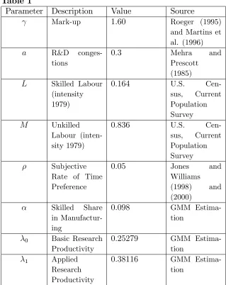
The following Table 1 reports the parameters we have utilised and their sources:
25Source: US Census - Current Population Survey, Annual Social and Economic
supple-ments.
Table 1
Parameter Description Value Source
Mark-up 1:60 Roeger (1995)
and Martins et al. (1996)
a R&D conges-tions
0:3 Mehra and
Prescott (1985)
L Skilled Labour
(intensity 1979)
0:164 U.S. Cen-sus, Current Population Survey
M Unkilled
Labour (inten-sity 1979)
0:836 U.S. Cen-sus, Current Population Survey Subjective
Rate of Time Preference
0:05 Jones and
Williams
(1998) and
(2000) Skilled Share
in Manufactur-ing
0:098 GMM
Estima-tion
0 Basic Research
Productivity
0:25279 GMM Estima-tion
1 Applied
Research Productivity
0:38116 GMM Estima-tion
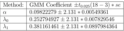
We have estimated the R&D and manufacturing technological parameters
0, 1 , and in the Public Basic Research scenario, by using the Generalised
Method of Moments28 (GMM) with data from 1963 to 198129. The reason
28The software we have used is E-views 6.
29We can safely use the 1981 data to measure the e¤ects of the "pre-1980" regime,
why we have also estimated parameter - the high skilled labour30 share in
manufacturing production - instead of relying on available statistics, is that they fail to single out the fraction of high skilled labour in production31, con-sistently with our stylized economy. Since we do not have data on variables
m(A0), nA, v0L, v1L, x, we have reduced system (8a)-(8g) by repeated
substi-tutions to only two equations32, and used these to estimate the parameters
with the remaining variables, ws, M, L,LG,gP U BBL, on which we have time
series from 1963 to 1981. The GMM estimator can deal with such highly non-linear equations, is consistent, and, more importantly, yields results ro-bust to heteroschedasticity and autocorrelation of unknown form (Hansen, 1982). In the estimates reported in Table 2 we had chosen the weighting
ma-trix in GMM-Time Series (HAC), with Newey and West …xed bandwidth33
Quite reassuringly, our results do not di¤er substantially34 when we use the
Two-Stage Instrumental Variable (IV) estimator, which may be desirable in small samples in case heteroschedasticity is not present. Similarly for the
Three-Stage IV estimators35. In all our GMM and IV regressions we have
used lagged innovation as an instrument.
In order to check the robustness of our simulations of the alternative scenarios, we have let our estimates vary on their 95% con…dence interval. In Table 2 we report the GMM estimated con…dence intervals for the estimated parameters:
30In this paper’s restrictive interpretation as highly skilled workers with at least college
education, and able to perform R&D activities competently.
31For example, the ratio of non-production workers in operating establishments to total
employment in 1979 was 0.248 (Berman, Bound, and Griliches, 1994), but this would include a large fraction of not highly skilled workers, as well as people actually undertaking knowledge-related activities.
32Reported in Appendix 3.
33But results only marginally changed when we used (as a robustness check) Andrews
and Variable Newey-West bandwidth selection. These are not reported in the paper to save space, but would not change the rankings of the simulated scenarios.
34They are almost identical even with simple Nonlinear Least Squares. Of course, the
GMM estimator is more e¢cient in the presence of arbitrary heteroschedasticity.
35With resulting estimates: ^
0 = 0:257987, ^1 = 0:387889, and ^ = 0:097176; and
Table 2
Method: GMM Coe¢cient t0:025(18 3) se
0:09822279 2:131 0:00549361
0 0:252794927 2:131 0:007829546 1 0:381161461 2:131 0:0897984364
wheret0:975(18 3)denotes the 97.5% value of the Student-t random
vari-able withT k = 15 degrees of freedom, andsedenotes the standard errors
of the estimate. All variables are highly signi…cant, and their 5% con…dence
interval are relatively small. We will use them, along with the other parame-ters taken from the literature, to compare the alternative policy scenarios.
5.3
Policy Comparisons
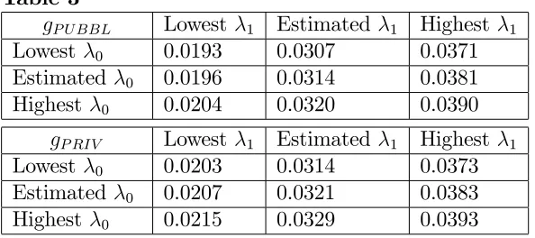
In this section we utilise the previously estimated values of the technolog-ical parameters as well as all the previously estimated exogenous to compute the hypothetical steady state equilibrium of the two scenarios - unpatentable research tools versus patentable research tools - for the year 1979, i.e. the last year of the non-patentable research tools regime. It is important to remark that the qualitative results do not change if instead we use any combinations of the data in the last 5 years time interval (from 1975 to 1979).
In our exercise, we compared the steady state equilibrium innovative per-formance of the patentable research tool scenario not only with the actual performance in those years, but also with a hypothetical public scenario constrained to employ the same number of basic researchers as would the privatize system have done. This allowed us to purge the comparison from di¤erent levels of employment and allows us to focus on the induced e¢-ciency gains from research tool patentability. In fact, the endogenous public sector ine¢ciency in channelling researcher’s e¤ort only in the sectors where …rms need a research tool is weighted against the under-incentive e¤ect of the patented research tools in the downstream research.
The following Table 3 lists the comparative innovation rates in the pri-vatized scenario and in the public basic research scenario, at the estimated coe¢cient values as well as at the lower and higher bounds of their 95%
on space, but results would not change much (certainly not the qualitative
ranking) if we had let take on other values in its 95% con…dence
inter-val. However, given their importance, we report the results associated with
the technological parameters 0 and 1. The upper part of Table 3 shows
how the balanced growth path aggregate innovation rate of the public basic
research economy, gP U BBL, changes over the 95% con…dence interval of the
parameters 0 and 1; while the lower part of Table 3 shows how the
bal-anced growth path aggregate innovation rate of the privatized basic research
economy, gP RIV, changes over the 95% con…dence interval of the parameters
[image:24.612.168.465.318.450.2]0 and 1.
Table 3
gP U BBL Lowest 1 Estimated 1 Highest 1
Lowest 0 0.0193 0.0307 0.0371
Estimated 0 0.0196 0.0314 0.0381
Highest 0 0.0204 0.0320 0.0390
gP RIV Lowest 1 Estimated 1 Highest 1
Lowest 0 0.0203 0.0314 0.0373
Estimated 0 0.0207 0.0321 0.0383
Highest 0 0.0215 0.0329 0.0393
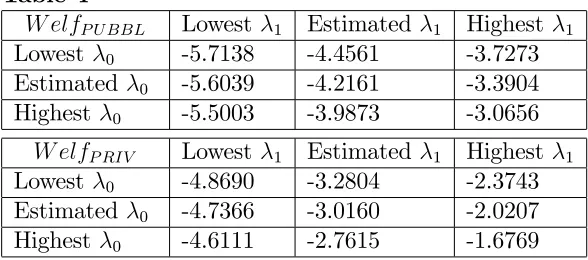
We have also simulated the welfare levels36
W elfs =
Z 1
0
e rt log( )g
st+ log(xsM1 ) dt=
= log( )gs
r2 +
log(xsM1 )
r ,s =P U BBL, and P RIV. (16)
associated with the di¤erent IPR scenarios. Notice that both the steady state
innovation rate, gs, and the steady state skilled manufacturing employment,
xs, can di¤er in di¤erent institutional scenarios s. More labour in research
would imply less manufacturing, with a negative level e¤ect on welfare, pos-sibly compensated by a positive growth e¤ect. Since the unskilled workers
are only employed in manufacturing, its level, M, does not change with s.
The simulated welfare values are shown in Table 4. The upper part of Table 4 shows how the balanced growth path welfare of the public basic
research economy, W elfP U BBL, changes over the 95% con…dence interval
of the parameters 0 and 1; while the lower part of Table 4 shows how
the balanced growth path welfare of the privatized basic research economy,
W elfP RIV, changes over the 95% con…dence interval of the parameters 0
[image:25.612.168.462.454.584.2]and 1.
Table 4
W elfP U BBL Lowest 1 Estimated 1 Highest 1
Lowest 0 -5.7138 -4.4561 -3.7273
Estimated 0 -5.6039 -4.2161 -3.3904
Highest 0 -5.5003 -3.9873 -3.0656
W elfP RIV Lowest 1 Estimated 1 Highest 1
Lowest 0 -4.8690 -3.2804 -2.3743
Estimated 0 -4.7366 -3.0160 -2.0207
Highest 0 -4.6111 -2.7615 -1.6769
The privatized basic research regime seems to dominate the public regime also in terms of welfare. Therefore the reader can notice from our tables that in 1979 the unpatentability of the basic scienti…c …ndings imposed more ine¢ciency to the US innovation system than would the monopolization of
applied research would have implied. The policy makers or the courts ended up acting as if they had been aware of this, thereby switching law and doctrine towards the patentability of research tools, inaugurated at the beginning of the Eighties. Therefore our analysis suggests that the policy change in favour of the research tools patentability occurred in the United States from the early Eighties was very likely to be the best institutional reaction to the increase in R&D complexity.
6
The Research Exemption Economy
A patent gives the inventor the exclusive rights to manufacture, use or sell the invention. But it is more important to stress that all these rights are
veto-rights: hence they can be exercised only if the patent holder is able to observe and sue the infringer of his/her patent. Unlike the production of new …nal products, which can be easily observed by someone who has a patent on it, the use of a speci…c research tool in the R&D of a new product can hardly be observed by third parties: its only output is the probability per unit time of innovating. More realistically, only after the innovation has actually appeared i.e. the corresponding …nal product gets patented and actually produced -will the research tool patent holder be able to e¤ectively exercise his power to sue, forcing the infringer who succeeded in innovating to share the pro…ts resulting from the sale of the …nal product. This kind of strategic R&D environment is known as "Research Exemption", and it is subject to intense
juridical controversies37, following the famous Supreme Court decision on
Madey v. Duke University suit, which practically eliminated the possibility
of appealing to it, except under very narrow circumstances. In cases where access to research tools through the marketplace is highly problematic, a research exemption is deemed desirable (Mueller, 2004).
Therefore, the privatized scenario of Section 4 corresponds to a an ex-treme case of perfect information and veri…ability of the unauthorized use of the patented research tool. Here, in order to assess the robustness of our pre-vious numerical results, we simulate would happen in another privatized case, but with imperfectly informed patent holders. With this aim, in this section we develop a third scenario that emphasizes the e¤ect of ex-post bargaining between an upstream patent holder and its downstream developer: an
in-37See Mueller (2004) for a detailed discussion of the research exemption debate in the
novation (a completed half idea) can be patented and yet infringe another patent (the patented research tool).
The new model of this section is inspired by Green and Scotchmer (1995),
which pioneered microeconomic research on this important issue38. In order
to cast their insight in our general equilibrium framework, we assume that the new …nal product is patentable but infringes its research tool. Ex post bar-gaining is rationally expected to transfer to the basic research patent holder a fraction 0< <1of the value of the …nal product patent, representing its relative bargaining power. Unlike Green and Scotchmer’s (1995) assumption of a unique downstream researcher, we here assume that the downstream unauthorized research with a patented research tools can be carried out by a multitude of freely entrant R&D …rms, thereby implying a demand e¤ect on R&D inputs dissipating expected pro…ts, and potentially depressing welfare. Our analysis is also valid in the case of reach-through licensing agreements, which seem pervasive in the US. "For research tools ... [r]oyalities would be pass-through royalties from the product developed to the tool." Maurer and Scotchmer (2004b, p. 236). We …rst analyze non-exclusive licenses, while the next subsection will study exclusive pass-through licensing agreements. In all our cases, we assume that the ultimate patent on the …nal product improvement can be granted to only one …rm: the …rst to invent it.
Let vB,vL0, and vL1 denote respectively the present expected value of a
basic blocking patent (vB), an A0 industry quality leader (v0L ), and an A1
industry challenged leader (v1
L).
Costless arbitrage between risk free activities and …rms’ equities imply that at each instant the following equations shall hold in equilibrium:
ws = 0nBavB (17a)
rvB = 1n1A a v
0
L vB +
dvB
dt (17b)
ws = 1nAa(1 )v0L (17c)
rv0L = n1 a B 0 v
0
L vL1 +
dv0
L
dt (17d)
rv1L = n1 a
A 1vL1 +
dv1
L
dt (17e)
Equation (17a) is the zero pro…t condition of a free entrant basic R&D
…rm in anA0 industry, equalizing the skilled wage and the probability 0nOa
of inventing a half idea times the value vB of the resulting blocking patent.
Equation (17b) states that …nancial arbitrage pins down the unique value
of the blocking patent that equals the risk free income from its sale, rvB,
to the expected present value of maintaining it in an A1 industry. These
are the expected increase in value deriving from someone else’s - the nA
downstream researchers’ - discovering the industrial application, plus the gradual appreciation in the case of someone else’s R&D success not arriving,
dvB dt .
Equation (17c) is the free entry condition for downstream completers that
rationally expect to appropriate only fraction 1 of the value of the …nal
good monopolist. Notice that unlike in Section 5, the expectation of ex-post bargaining or the presence of reach-through licenses introduces a negative incentive e¤ect of downstream innovation, because the infringer’s use of a research tool can appropriate only a fraction of the value of its marginal product.
The last two equations have the usual interpretation.
It is important to note that our results do not hinge on assuming that the …rst stage patent holder undertakes no applied R&D. In fact, the free entry condition (17c) dissipates all excess pro…ts from doing so: the research tool patent holder, by hiring a marginal unit of skilled labour to complete its patent would increase its expected gains by 1nAa(1 )v0L ws= 0. Hence,
it would just be equivalent to one of the free entrants into downstream R&D. Therefore, our model is consistent with an indeterminate R&D participation of the …rst stage blocking patent holder.
It is also important to notice that free entry into downstream research vani…es any attempt to resort to ex ante licensing, which would instead hold if, as Green Scotchmer (1995), Scotchmer (1996), Denicolo (2000), and Aoki and Nagaoka (2007), we had restricted entry to the second stage of R&D to only one completing …rm.
As in the previous sections, the industrial dynamics of this economy is described by the following …rst order ordinary di¤erential equation:
dm(A0)
dt = (1 m(A0)) 1(nA)
1 a
m(A0) (nB)1 a 0. (18)
These equations, supplemented with the skilled labour market equilibrium condition
and by eq. (11) for x determine the equilibrium trajectories.
Since is either regime there is free entry into one of the two types of research activities, this may lead to excessive entry into basic research in the private regime, and excessive entry into development in the public regime, and potentially too in this section’s private regime, due to the absence of a market for basic ideas. While the lack of commercial focus in basic research can make publicly funded research worse, excessive entry into basic research in the private regime can potentially counter this handicap. Hence, it is not possible a priori to rank the two regimes. This makes a numerical analysis based on estimated parameters compelling.
We utilise the previously estimated values of the technological parame-ters as well as all the previously described relevant exogenous parameparame-ters to compute the hypothetical steady state equilibrium of the two scenarios - unpatentable research tools versus patentable research tools - for the year 1979, the last year of the non-patentable research tools regime. It is im-portant to remark that our comparisons would not change if instead we use any combinations of the data in the last 5 years time interval (from 1975 to 1979). The aggregate innovation rate in this economy is denoted
gREx (1 m(A0)) 1(nA)
1 a
. This expression will be used in all simula-tions.
6.1
Balanced Growth Path
Also in this economy, in a balanced growth path equilibrium all variables are constant except the average quality of consumer goods, and therefore the instantaneous percapita utility index, which grows at a constant rate
ln( )gRExproportional to the aggregate innovation rategREx=m(A0) (nB)1 a
0 =
(1 m(A0)) 1(nA)
1 a
. Based on the previous characterization, we can
state:
De…nition 3. A balanced growth path equilibrium of the Research Ex-emption economy is a vector [m(A0); nB; nA; vB; vL0 v1L; ws; x; gREx]2R9+
ws = 0nBavB (20a)
rvB = 1n1A a v0L vB (20b)
ws = 1nAa(1 )vL0 (20c)
rvL0 = n1 a B 0 v
0
L vL1 (20d)
rvL1 = n1 a A 1v
1
L (20e)
(1 m(A0)) 1(nA)1 a
= m(A0) (nB)1 a
0 (20f)
L = x+m(A0)nB+ (1 m(A0))nA (20g)
x = 1
ws 1
M (20h)
gREx = (1 m(A0)) 1(nA)1 a
. (20i)
Due to the analytical complexity of such system, also in this case we resorted to numerical analysis. In all numerical simulations we have run, the steady state exists, and it is saddle point stable for any set of parameter values. Therefore, given an initial condition form(A0), there is (locally) only
one initial condition for v0
L, vL1, and vA such that the generated trajectory
tends to the steady state vector: the equilibrium is determinate.
Since, in principle, our numerical simulations could converge to just one of possibly many di¤erent steady states, the empirical calibrations and policy conclusions we could obtain would not be credible unless we can …rst prove analytically the uniqueness of the steady state in the model we are using. This is achieved by the following:
Lemma 3. In the Research Exemption economy there can exist no more than one balanced growth path equilibrium.
Proof. See Appendix 2.
6.2
Numerical Comparisons
In this section, we compare the steady state equilibrium innovative per-formance of the patentable research tool scenario with a hypothetical public scenario constrained to employ the same number of basic researchers as in the private equilibrium. As in Scotchmer and Green (1995) and Scotchmer
(1996), we set parameter = 0:5.
1. GMM estimation of the values of the unobservable parameters , 0
and 1 based on U.S. 1963-1980 data: results in Table 2.
2. Use of the estimated parameter values ^, ^0 and ^1, along with other
parameters shown in Table 1 in the system of equations of the balanced growth path equilibrium of the Research Exemption Economy.
3. Use of the previous parameters and of the steady state equilibrium amount of basic research labour, m(A0)nB, estimated in Step 2 into
the Public Basic Research Economy scenario, setting LG = m(A0)nB,
and simulation of the corresponding Public Basic Research Economy scenario.
4. Comparison of the steady state innovation rates and welfare levels of the two policy scenarios of steps 2 and 3.
The following Table 5, lists the comparative innovation rates in the pri-vatized scenario and in the public basic research scenario, at the estimated coe¢cient values as well as at the lower and higher extremes of their 95% con…dence intervals. We report the results associated with the technological
parameters 0 and 1, which the reader can …nd in Table 2. The upper part
of Table 5 shows how the balanced growth path aggregate innovation rate
of the public basic research economy, gP U BBL, changes over the 95%
con…-dence interval of the parameters 0 and 1; while the lower part of Table
5 shows how the balanced growth path aggregate innovation rate of the
re-search exemption economy, gREx, changes over the 95% con…dence interval
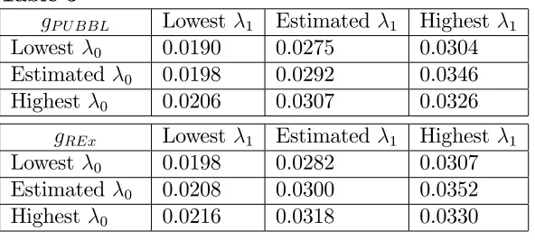
[image:31.612.169.465.550.683.2]of the parameters 0 and 1.
Table 5
gP U BBL Lowest 1 Estimated 1 Highest 1
Lowest 0 0.0190 0.0275 0.0304
Estimated 0 0.0198 0.0292 0.0346
Highest 0 0.0206 0.0307 0.0326
gREx Lowest 1 Estimated 1 Highest 1
Lowest 0 0.0198 0.0282 0.0307
Estimated 0 0.0208 0.0300 0.0352
As the data in the table show, the privatized basic research scenario with the possibility of downstream researchers carrying out R&D and infringing the upstream patent holder outgrows the public basic R&D scenario for all combinations of the underlying technological parameters over their 95% con-…dence interval.
Also in this case we have also simulated the welfare levels
W elfs =
Z 1
0
e rt log( )gst+ log(xsM1 ) dt =
= log( )gs
r2 +
log(xsM1 )
r , s=P U BBL, and REx. (21)
associated with the di¤erent IPR scenarios. Notice again that both the steady state innovation rate,gs, and the steady state skilled manufacturing
employ-ment, xs, can di¤er in di¤erent institutional scenarios s.
The simulated welfare values are shown in Table 6. The upper part of Table 6 shows how the balanced growth path welfare of the public basic
research economy, W elfP U BBL, changes over the 95% con…dence interval of
the parameters 0 and 1; while the lower part of Table 6 shows how the
balanced growth path welfare of the research exemption economy,W elf REx,
[image:32.612.171.464.440.571.2]changes over the 95% con…dence interval of the parameters 0 and 1.
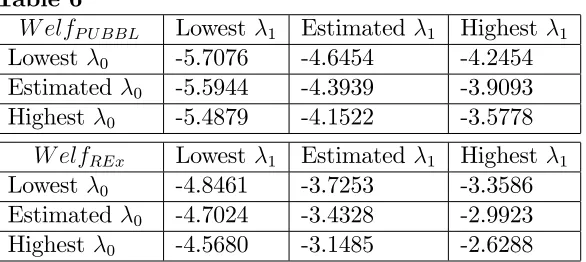
Table 6
W elfP U BBL Lowest 1 Estimated 1 Highest 1
Lowest 0 -5.7076 -4.6454 -4.2454
Estimated 0 -5.5944 -4.3939 -3.9093
Highest 0 -5.4879 -4.1522 -3.5778
W elfREx Lowest 1 Estimated 1 Highest 1
Lowest 0 -4.8461 -3.7253 -3.3586
Estimated 0 -4.7024 -3.4328 -2.9923
Highest 0 -4.5680 -3.1485 -2.6288
This research exemption and/or reach-through agreements analysis is therefore quite important in assessing the robustness of our previous results, in favour of the US policy shift towards the patentability of basic knowledge in 1980.
7
Final Remarks
The debate on the e¤ects of the patentability of research tools on the in-centives to innovate is still very controversial, not only in the US but also in Europe and in other important areas of the world. This paper analyzed from a general equilibrium perspective the US policy shift towards the extension of patentability to research tools and basic scienti…c ideas that took place around 1980. These normative innovations have been modifying the indus-trial and academic lives in the last three decades, raising doubts on their desirability. The losses from the free entry into basic research and the mo-nopolization of applied research induced by intellectual property of research tools have been compared with the ine¢cacy of public research institutions to promptly react to downstream market opportunities and the potentially excessive entry into applied R&D.
Results were not a priory unambiguous, which forced us to use the avail-able data and calibrate and simulate our model in order to check if the US did it right in changing their institutions around 1980. We have robustly found that assigning property rights to basic research …ndings and creating a market for research tools was the best thing the US could do at that time. We have extended the basic model to incorporate research exemptions and reach-through licensing, without modifying our main policy conclusions. In light of the current international negotiations on the application of TRIPs, our analysis might be helpful in providing insights from the experi-ence of an important turning point in the US national system of innovation.
8
Bibliography
Aghion, P. and Howitt, P. (1992), “A Model of Growth through Creative
Destruction”, Econometrica 60 (2), p. 323-351;
Aghion, P. and Howitt, P. (1998), “Endogenous Growth Theory”, MIT Press;
Aoki, R. and Nagaoka, S. (2007), "Economic Analysis of Patent Law
Exemption for Research on a Patented Innovation", Institute of Innovation
Research, Hitotsubashi University, working paper.
Berman, E., J. Bound, and Z. Griliches, (1994), "Changes in the Demand for Skilled Labor within U.S. Manufacturing: Evidence from theAnnual
Sur-vey of Manufacturers", The Quarterly Journal of Economics, Vol. 109, No.
2, pp. 367-397.
Bramoulle’, Y. and G. and Saint-Paul’s (2010), "Research Cycles", Jour-nal of Economic Theory, 145, pp.1890–1920.
Denicolò, V. (2000), "Two-Stage Patent Races and Patent Policy ",RAND Journal of Economics, vol. 31, 3, pp. 488-501;
Denicolò, V. (2007), "Do patents over-compensate innovators? ", Eco-nomic Policy, Vol. 22 Issue 52 Page 679-729;
Dinopoulos, E. and Thompson, P.S., (1998), “Schumpeterian Growth
Without Scale E¤ects”, with Peter Thompson,Journal of Economic Growth,
3, pp. 313-335.
Dinopoulos, E. and Thompson, P. S., (1999), “Scale E¤ects in
Neo-Schumpeterian Models of Economic Growth”, Journal of Evolutionary
Eco-nomics, 9(2), pp. 157-186.
Gersbach, H., G. Sorger, and C. Amon (2009), "Hierarchical Growth: Basic and Applied Research ", Center of Economic Research at ETH Zurich, Working paper No. 09/118
Green, J. and Scotchmer, S. (1995)."On the Division of Pro…t in Sequen-tial Innovations", The Rand Journal of Economics 26, pp. 20-33
Griliches, Z. (1990), "Patent Statistics and as Economic Indicators: A Survey", Journal of Economic Literature, 18(4), pp. 1661-1707.
Grossman, G.M. and Helpman, E. (1991a), “Quality Ladders in the
The-ory of Growth”, Review of Economic Studies 58, pp. 43-61;
Grossman, G.M. and Helpman, E. (1991b),Innovation and Growth in the
Global Economy, MIT Press, Cambridge, MA.
Grossman, G.M. and Shapiro, C. (1986), “Optimal Dynamic R&D
Pro-grams”, RAND Journal of Economics 17, 4, pp. 581-593;
Grossman, G.M. and Shapiro, C. (1987), “Dynamic R&D Competition”,
The Economic Journal 97, pp. 372-387;
Howitt, P. (1999), "Steady Endogenous Growth with Population and R&D Inputs Growing", Journal of Political Economy, vol.107, n. 4, pp.715-30;
Jensen, R. and Thursby, M. (2001), "Proofs and Prototypes for Sale: The Licensing of University Inventions", American Economic Review, 91(1), pp. 240-59;
Jones, C., (1995) “R&D-Based Models of Economic Growth ”, Journal
of Political Economy, 103: 759-784;
Jones, C. and J. Williams (1998), "Measuring the Social Return to R&D",
Quarterly Journal of Economics, November 1998, Vol. 113, pp. 1119-1135. Jones, C. and J. Williams (2000), "Too Much of a Good Thing? The
Economics of Investment in R&D", Journal of Economic Growth, March
2000, Vol. 5, No. 1, pp. 65-85.
Jones, C., (2005)”Growth in a World of Ideas”, in P. Aghion and S. Durlauf (eds.) Handbook of Economic Growth (Elsevier, 2005) Volume 1B, pp. 1063-1111.
Krusell, P., L. Ohanian, J.V. Rios-Rull and G. Violante (2000):
“Capital-Skill Complementarity and Inequality”, Econometrica, 68:5, 1029-1054.
Leiva-Beltran, Fernando (2007), "Research vs. Development", University of Iowa working paper.
Madsen, J. B., (2008), "Semi-endogenous versus Schumpeterian growth models: testing the knowledge production function using international data",
Journal of Economic Growth, 3.1, pp. 1-26.
Martins, J. Scarpetta, S. and D. Pilat, (1996),. ”Markup Pricing, Market
Structure and the Business Cycle”, OECD Economic Studies 27, 71-105;
Maurer, S. M. and Scotchmer, S. (2004a), "A Primer for Nonlawyers on Intellectual Property", in Scotchmer, S. (2004), "Economics and Incentives", MIT Press, Cambridge, Ma., p.65-95.
Maurer, S. M. and Scotchmer, S. (2004b), "Innovation Today: A Private-Public Partnership", in Scotchmer, S. (2004), "Economics and Incentives", MIT Press, Cambridge, Ma., p.227-258.
Mehra, R. and E.C. Prescott, (1985) “The Equity Premium: A Puzzle”,
Journal of Monetary Economics 15, 145–161.
Mueller, J. M. (2004), "The Evanescent Experimental Use Exemption from United States Patent Infringement Liability: Implications for University
and Nonpro…t Research and Development", Baylor Law Review, 56, p.917.
Peretto, P., (1998), "Technological Change and Population Growth",
Journal of Economic Growth, 3, pp. 283-311.
Reinganum, J. (1985), "A Two-Stage Model of Research and
Develop-ment with Endogenous Second Mover Advantages",International Journal of
Industrial Organization, 3, p. 275-292.
Roeger, W. (1995). “Can Imperfect Competition Explain the Di¤erence between Primal and Dual Productivity Measures? Estimates for US
Manu-facturing”, Journal of Political Economy 103, 2, 316-330;
Scotchmer, S. (1996), "Protecting Early Innovators: Should Second-Generation
Products Be Patentable?, RAND Journal of Economics, vol. 27, pp. 29-41.
Scotchmer, S. (2004), "Economics and Incentives", MIT Press, Cam-bridge, Ma.
Segerstrom, P.S. (1998), “Endogenous Growth Without Scale E¤ects,”
American Economic Review, vol. 88,n. 5, pp.1290-1310;
US Census (2010a), Current Population Survey, Historical Tables. US Census (2010b), Current Population Survey, Annual Social and Eco-nomic supplements.
USPTO (2010), US Patent Statistics Chart - Calendar Years 1963-2010, U.S. Patent and Trademark O¢ce.
Young, A. (1998), "Growth without Scale E¤ects", Journal of Political Economy, 106, 41–63.
Appendix 1
Model Details
This Appendix explains the details of the quality ladder model used in the main taxt. It may be skipped by most readers familiar with this literature.
Time t 0population P(t) is assumed growing at rategP op 0 and its
initial level is normalized to1. The representative household preferences are represented by the following intertemporally additive utility functional39:
U =
Z 1
0
e rtlnD(t)dt, (22)
39We skip starting with an expectational operator in order to save notation. A more